2.1 The RV Investigator and the voyage

The RV Investigator is an ocean research vessel configured to enable a wide range of atmospheric, biological, geoscience and oceanographic research. The vessel is 94 m long, has a gross weight of 6082 tons and has a fuel capacity of 700 tons of ultra-low sulfur diesel fuel. It is powered by three 9-cylinder 3000 kW MaK diesel engines, each coupled to a 690 V AC generator. Ship propulsion is achieved using two 2600 kW L3 AC reversible propulsion motors powered by these generators. The RV Investigator can host up to 30 crew members and 35 researchers for a maximum voyage period of 60 days, with a maximum cruising speed of 12 knots.

A suite of instrumentation for atmospheric research is available on the RV Investigator. This includes a radar system capable of collecting weather information within a 150 km radius of the vessel, and instruments measuring sunlight parameters; aerosol composition, particle concentration and size distributions; cloud condensation nuclei; gas concentrations; and various other components of the atmosphere. These instruments are housed inside two dedicated on-board laboratories for aerosol and for atmospheric chemistry research. An atmospheric aerosol sample is continuously drawn into the laboratories for analysis through a specialized inlet fitted to the foremast of the ship. Of particular interest to this study is that the ship contains a PICARRO (PICARRO Inc., Santa Clara, California, USA) G2401 analyser that continuously measures CO₂, CO, H₂O and CH₄. It has an operation range between 0 and 1000 ppm and a parts-per-billion (ppb) sensitivity for CO₂.

The 2-day UAV measurement study was possible as part of the RV Investigator voyage “The Great Barrier Reef as a significant source of climatically relevant aerosol particles”, which started in Brisbane on the 28 September 2016. The ship was used as both a floating platform to allow launch and recovery of the UAV system and as the source of an exhaust plume measured by the UAV system for EF calculation. During a stationary period several days long on the Great Barrier Reef off the coast of Australia, it was possible to measure the ship plume under stable real world conditions over two consecutive days. One of the three ship engines was maintained at a steady engine load of 25 %–30 % of the maximum engine power during all measurements.

2.2 UAV system

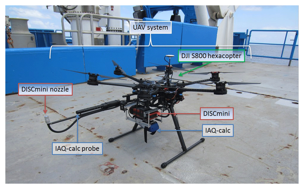
Measurements of PN and CO₂ concentrations in the ship plume were performed using two commercial sensors mounted on board a hexacopter UAV. The UAV used (Fig. 1) is a composite material S800 EVO manufactured by DJI (DJI, 2014). The UAV is 800 mm wide and 320 mm high, with an unloaded weight of 3.7 kg. Minimum and maximum take-off weights are 6.7 and 8 kg, respectively. The UAV contains a 16 000 mAh LiPo 6 cell battery, which provides a hover time of approximately 20 min when operating at minimum take-off weight. The telemetry range of the UAV is 2 km, which was adequate to cover the desired sampling area (see Fig. 2).

The payload consisted of a PN concentration and a CO₂ monitor mounted on board underneath the UAV. Careful placement of the payload was required to prevent flight issues caused by an altered centre of gravity. Also included was a carbon fibre rod, which extended outward horizontally from the UAV. The sampling lines for the monitors were attached to the end of this rod to ensure that measurements were not affected by the downwash of the UAV rotors. The total weight of the payload was 1.2 kg, which allowed the UAV system to fly for 12–15 min before landing at the home point (A) (see Fig. 2).

The S800 was used in conjunction with the DJI Wookong autopilot. The software provides an intuitive and easy-to-use interface in which autonomous flight paths can be planned, saved and uploaded into the UAV. In addition to this, the ground station allows for continuous, real-time monitoring of the status of the UAV during operation, which includes its longitude, latitude, altitude, waypoint tolerance and airspeed.

The DJI S800 was chosen for this study because it is designed to operate under the 20 kg all-up weight class of UAV. This reduces operational costs and avoids subjection to the tighter regulations of larger platforms. Small UAVs cannot be operated above any person or closer than 30 m to populated areas, houses and people. Furthermore, current Civil Aviation Safety Australia (CASA) regulations restrict the use of small UAVs (2 and 20 kg) to visual line-of-sight daylight operation, with a maximum altitude of approximately 120 m and within a radius of 3 nmi of an airport. UAVs in this category are not permitted for research unless the research institution has been granted a permit exception. These exceptions can be granted if the institution in question has or collaborates with an UAV operation team who must have an experienced UAV pilot who is also a radio controller specialist, a license for commercial UAV operation and appropriate liability insurance (CASA, 2014). Queensland University of Technology (QUT) has an unmanned operator certificate and four pilots who have UAV controller licenses.

Instrumentation for CO₂ concentration measurements

A TSI (TSI, Shoreview, Minnesota, United States) IAQ-calc 7545 model was chosen to measure CO₂ concentrations. Its sensor is based on a dual-wavelength NDIR (non-dispersive infrared) with a sensitivity range between 0 and 5000 ppm and an accuracy of ±3.0 % of reading or ±50 ppm (whichever is greater). The measurement resolution is 1 ppm with a maximum time resolution of 1 s. Similar to the DISCmini, the advantages of using the IAQ-calc are its small dimensions (178 mm × 84 mm × 44 mm); low weight (270 g, with batteries, significantly lower than the DISCmini); and a battery life of 10 h.

The readings of the IAQ-clac for CO₂ were compared with those measured by the on-board PICARRO G2401 analyser.

Both the DISCmini and the IAQ-calc were tested and calibrated in the on-board laboratory using ambient aerosol measurements at sea prior to the commencement of the measurements (Fig. S2 in the Supplement). All data were logged with a 1 s time interval.

Figure 1The UAV system with the on-board instrumentation: the DISCmini and the IAQ-calc.

Download

2.3 Meteorological data

Meteorological data (including air temperature, relative humidity, atmospheric pressure and wind speed and direction) were recorded by the RV Investigator's on-board instrumentation during the entire voyage with a 60 s time interval, 24 h a day.

2.4 Study design

During the two measurement days of this study, the vessel was heading into the wind whilst idling the UAV missions at sea. This positioning caused the exhaust plume to extend downwind, directly behind the ship. The UAV system was launched off the back deck, autonomously sampling at varying altitudes and distances into the downwind plume. Flight speed of the UAV was 1.5 m s⁻¹, the minimum for the S800.

Day 1 was used to optimize the study design, focusing on finding the flight path most suitable to capture the ship plume. Figure 2 shows the programmed flight path, which consisted of a continuous flight beginning at a distance (D) and from an altitude (H) above the surface. Point A, located on the back deck of the RV Investigator, represents the home point. In UAV terminology this refers to the position where the UAV system takes off and lands. The UAV system was programmed to move horizontally by a distance (2 d), perpendicular to the ship, then climb vertically for 10 m (h) before flying in the opposite horizontal direction for the same distance (2 d). The UAV was then programmed to climb another 10 m (h) before repeating this pattern until the UAV reached an altitude of 65 m above the ocean. During day 1, the UAV system followed three different flight paths, each one with both a different distance D behind the ship (20, 50 and 100 m) and a different horizontal distance 2 d (50, 100 and 150 m).

The optimized flight path for day 2 started 20 m behind the ship and 25 m above the surface, with no altitude variation. The UAV path was limited to a continuous horizontal flight of 50 m (2 d) at a steady speed of 2 m s⁻¹. This path and flying speed allowed up to four horizontal transects to capture the ship plume.

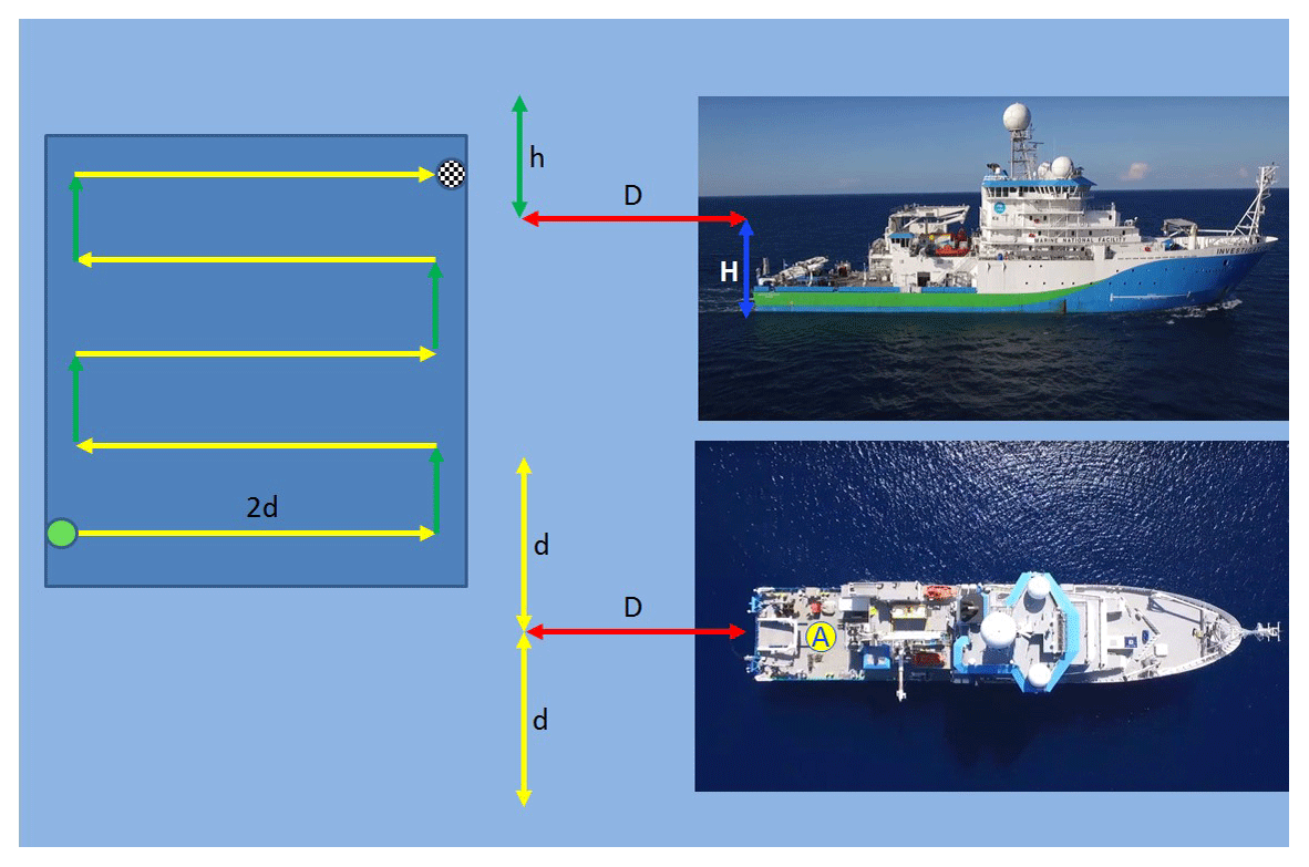
Figure 2Flight path used to capture the plume: H – height from the ocean, D – distance behind the ship to the flight beginning point, h – rising altitude after the horizontal transect, 2 d – full length of the horizontal transect.

Download

2.5 Experimental procedure

The UAV can fly either manually or autonomously. As a safety precaution, every take-off and landing was performed using the manual flight mode. Once in the air, the UAV was switched to autonomous flight mode, allowing the platform to follow the preprogrammed flight path discussed in the previous section. The flight path consisted of waypoints, which are three-dimensional GPS points that dictate the position of the UAV along the fight path. The waypoints and flight plans for each flight were programmed using the aforementioned DJI Wookong ground station software. The DISCmini and the IAQ-calc were fitted on the underside of the UAV at the beginning of each measuring day. Five flights were performed across the two measurement days, providing a total of 27 horizontal transects perpendicular to the ship's exhaust plume.

2.6 Emission factors

The calculation of an emission factor for particle number concentration (EF_PN) from the collected ship plume measurements was performed using Eq. (1). This method has previously been used for ship (Westerlund et al., 2015), road vehicle (Hak et al., 2009) and aircraft (Mazaheri et al., 2009) emissions. The measured values of PN concentration were related to the amount of fuel consumed by the engine in question through the use of the simultaneous measurements of CO₂ concentration taken by the UAV. This was achieved by using a published value for a ship emission factor of CO₂ (EF_gas) of 3.2 kg CO₂ (kg_fuel)⁻¹ (Hallquist et al., 2013; Hobbs et al., 2000).

The ΔPN and Δgas in Eq. (1) represent the maximum particle concentration change above background in the measured particle number and CO₂ concentrations, respectively. The DISCmini measurements were corrected against a reference condensation particle counter (CPC). For each transect data series of PN concentration and CO₂, the averaged background concentrations were subtracted from the peak data corresponding to measurements inside the plume. The corrected peak data series were then fit with a Gaussian curve using the inbuilt Matlab curve fitting application. The least absolute residuals condition was used as this most closely fits the curve to the highest magnitude data points in the series. The maximum peak heights of the fitted Gaussian curves were used as ΔPNC and ΔCO₂ in the calculation of emission factors for each transect.

3.1 Meteorological and Investigator data

Wind conditions were very stable during both day 1 and 2, following one main pattern for the entire flight time. The wind speed ranged from 3 to 13 m s⁻¹. The wind direction was predominantly from the NE during day 1 and ESE during day 2. The wind rose graphs in Fig. 3a and b illustrate the wind data recorded with the on-board weather instrumentation during all horizontal transects flown during day 1 and 2 respectively. The prevalent wind direction was ESE, which corresponded to the heading of the RV Investigator (indicated by the rose triangle). The wind direction changed occasionally to E during the flight, causing the UAV to fail to capture the RV Investigator plume during some transects. As a result, two of the eight horizontal transects collected on day 2 were excluded from the analysis.

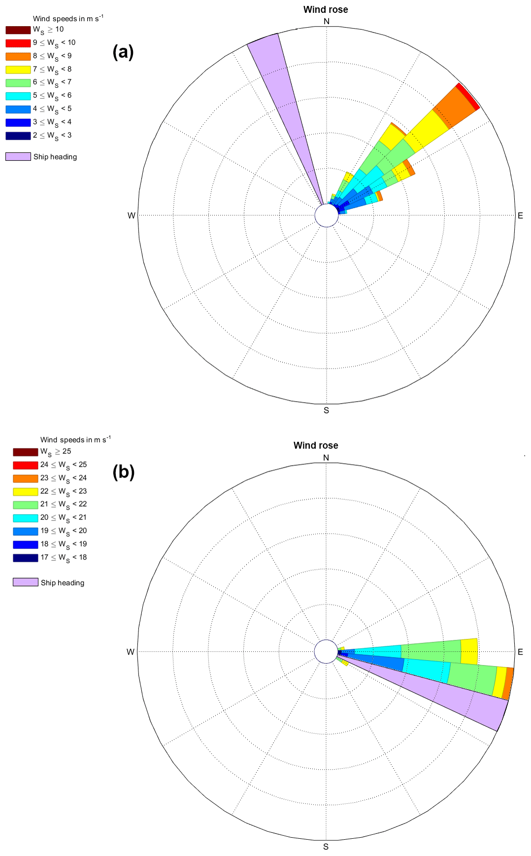
Figure 3Wind rose showing wind speed and direction during optimized flight paths for day 1 (a) and day 2 (b). The rose triangle shows the direction of RV Investigator during the measurements.

Download

3.2 UAV system horizontal transects inside and outside the plume

The UAV system acquired data for a total of 27 horizontal transects for day 1 and 2. Data were collected at altitudes between 25 and 65 m above the water surface. During day 1 the plume was captured once when the UAV was at 25 m altitude and 20 m downwind of the ship, and again at both 25 and 35 m altitude 100 m downwind of the ship. These observations led to the optimized flight used on day 2, which started downwind at 25 m above the surface and 20 m behind the ship. On day 2 the UAV system successfully captured the plume during six of the eight transects performed. Across the 2 days, this led to a total of nine transects that captured the plume and which have been considered for discussion, shown in Table 1.

Table 1Specifications of the transects considered for the data analysis.

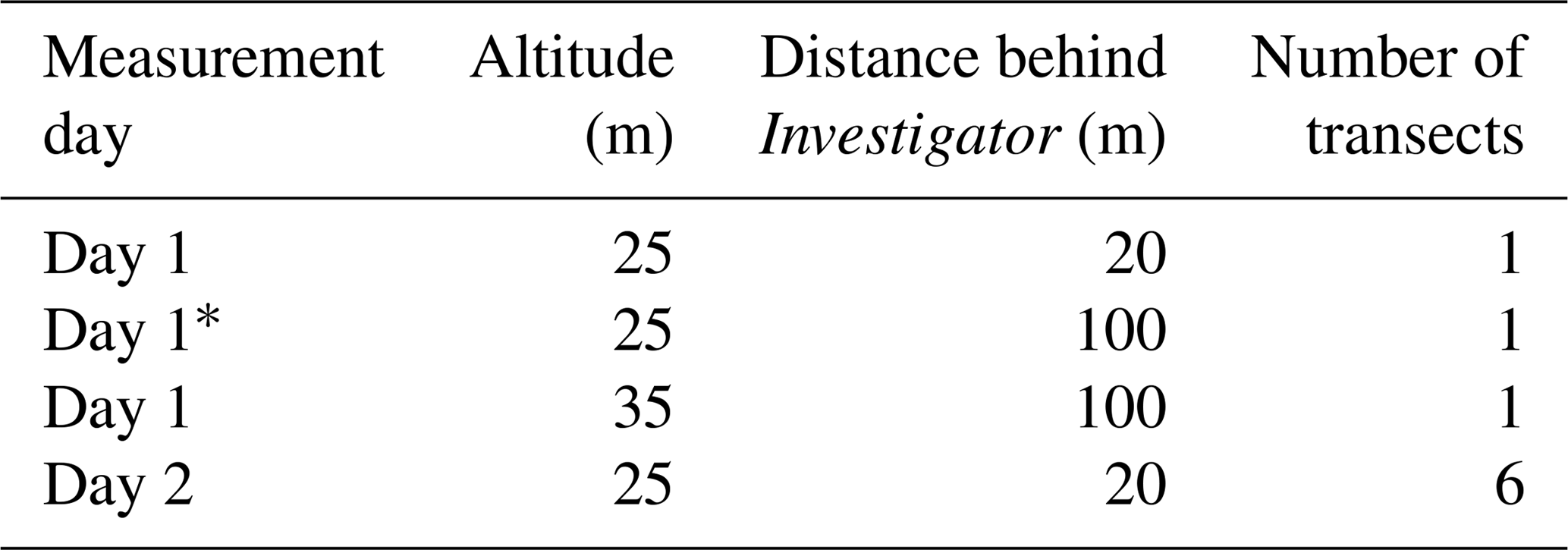
^* indicates the transect of Day 1 of which PN concentration and CO₂ profiles are presented in Fig. 4.

Download Print Version | Download XLSX

Figure 4 shows the PN concentration and CO₂ profiles, collected during two (a, b) transects on day 2 and (c) during one transect of day 1 (spec. in Table 1, Day1*).

The PN concentration profiles for the (a) and (b) transects in Fig. 4 show that the concentration varied by 5 orders of magnitude between the outside and inside of the plume, while the CO₂ profiles show an increase of up to 140 ppm above the background.

The profiles in (c) show that the PN concentration was 4 orders of magnitude greater inside the plume 100 m behind the ship and that the CO₂ concentration was up to 70 ppm higher inside the plume.

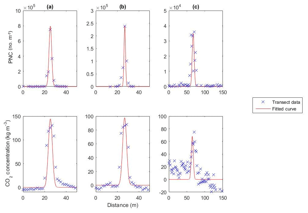
Figure 4Panels (a) and (b) show the measured PN and CO₂ concentration profiles and fitted Gaussian curves for two different transects 20 m behind the ship, 25 m above the surface during day 2. Panel (c) shows the PN and CO₂ concentration profiles and fitted Gaussian curves collected during flight 3 of day 1 100 m behind the ship, 25 m above the surface.

Download

Figure 4a and b both show transects at 25 m altitude and 20 m behind the ship. Both the PN concentration and CO₂ measurements show clear, single peaks as the UAV crosses the plume. As a consequence, these transects show a good fit with the corresponding Gaussian distribution curves, with R² values of above 0.9 for both PNC and CO₂. In contrast, Fig. 4c shows substantially less defined, wider peaks with lower pollutant concentrations. This is attributed to a difference in flight paths, with Fig. 4c representing data from a transect 100 m behind the ship. The additional time between emission and sampling has allowed the plume to broaden, become less homogenous and take on a skewed cross section. This results in a significantly lower R² value for the fitted Gaussian curves, with a value of 0.4998 for the CO₂ data in this transect. Therefore, whilst the 100 m transect does provide more data points inside the plume, the randomized variations inside the plume lead to less accurate calculations of emission factors.

Of further note in Fig. 4, the maximum PN concentration measured in (a) (7.5×10⁵ no. cm⁻³) is approximately 3 times greater than that in (b) (2.4×10⁵ no. cm⁻³), and the CO₂ concentrations in (a) are 43 ppm greater than (b). The transect flight plan and ship engine load remained constant throughout these measurements. The variations between (a) and (b) are attributed to several factors which reduce the effectiveness of the UAV transect for capturing the plume. Slight changes in ambient conditions such as temperature, wind direction and intensity will alter the path of the plume as it moves away from the ship. The UAVs' automated flight path cannot account for these variations. Therefore, the degree to which the UAV enters the plume, and thus the concentrations it measures, will be different on each transect. Both CO₂ and PN concentration measurements will be similarly affected by this variance. However, differences in instrument response rates in conjunction with these variances will be one of the major contributors to variations in calculated emission factors.

3.3 PN emission factors

Table 2 shows the distance and altitude of each transect, the R² values of the fitted Gaussian curves for PNC and CO₂ data, the calculated values of ΔPNC and ΔCO₂ and the calculated EF_PN.

Figure 5(a) ΔPNC against ΔCO₂ with a 95 % confidence interval for the six transects considered for the data analysis. (b) ΔPNC against ΔCO₂ with a 95 % confidence interval with the removal of the outlier transect from the first flight of day 2.

Download

Table 2Transect flight days and details, R² values for the Gaussian curve fits to both PNC and CO₂ data, ΔPNC and ΔCO₂ concentration emission/rate of the RV Investigator and calculated emission factors for PN.

Download Print Version | Download XLSX

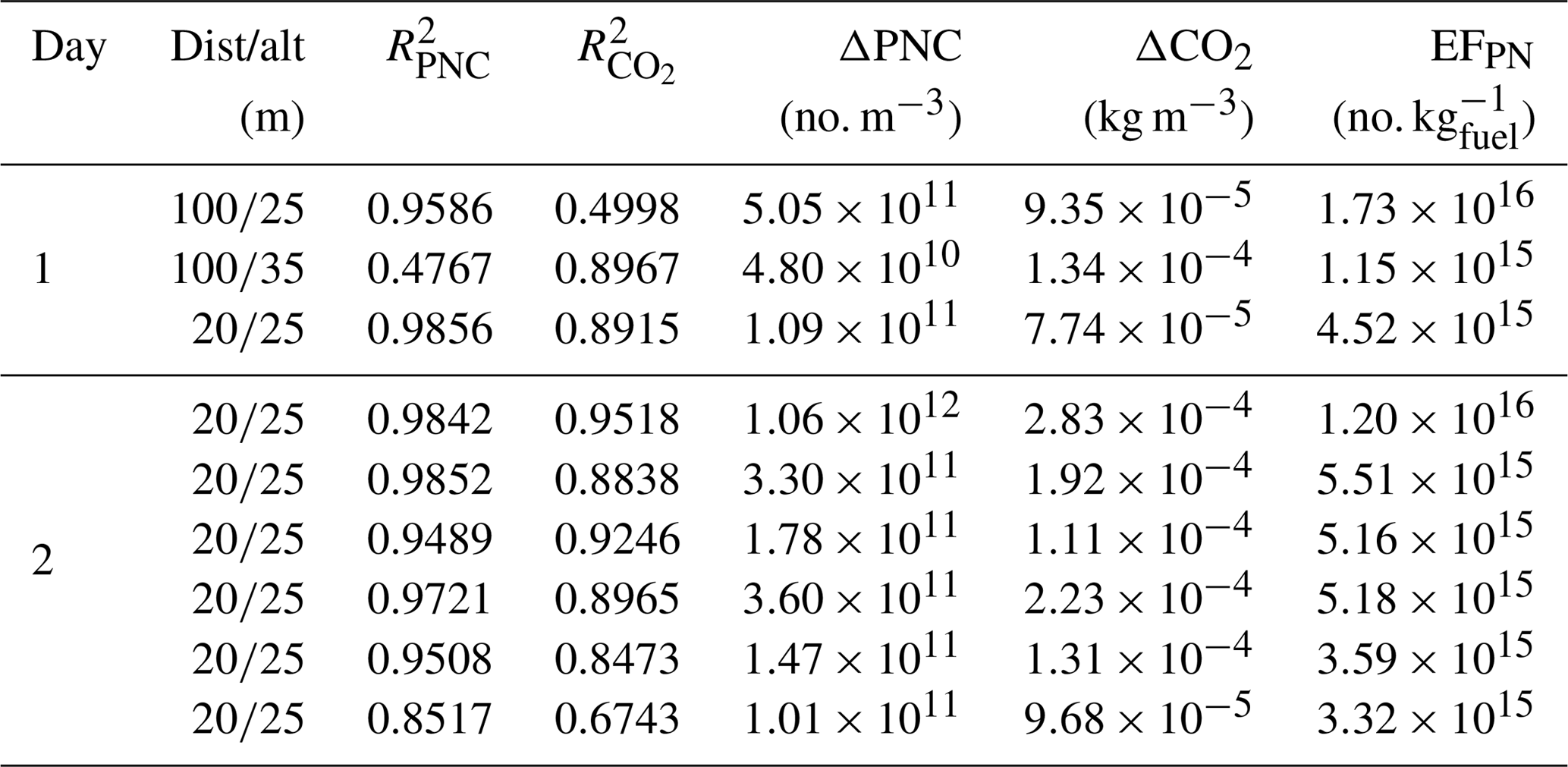
The calculated EF_PN values for the RV Investigator ranged from 1.15×10¹⁵ to 1.73×10¹⁶ no. kg${}_{\mathrm{fuel}}^{-\mathrm{1}}$. The two 100 m transects provided the worst Gaussian fits as well as the highest and lowest calculated emission factors. This indicates that it is important to filter out transects with data which do not fit the expected Gaussian distribution suitably as they can generate significant error. To this end, the 100 m transects were excluded from further analysis. ΔPNC and ΔCO₂ values for remaining transects were plotted against each other as shown in Fig. 5.

Figure 5a and b show the plots of the remaining transects ΔPNC against ΔCO₂ with and without the values of the first flight of day 2. This transect represents a clear outlier in the linear trend, with the R² value of the linear fit increasing from 0.637 to 0.890 with its exclusion. Furthermore, whilst the linear fit falls within the confidence interval of only one point in (a), it falls within all data points' confidence intervals in (b). This occurs despite both R² values for the fitted Gaussians of this transect being very high ($R_{\mathrm{PNC}}^{\mathrm{2}}=\mathrm{0.9842}$, $R_{{\mathrm{CO}}_{\mathrm{2}}}^{\mathrm{2}}=\mathrm{0.9518}$). This highlights a limitation with this methodology which can be best observed in the difference between Fig. 4a and b. The combination of UAV velocity, sampling rate and response time of the DISCmini results in the PNC transect data having only one data point defining the peak height of the transect. Relying on a single sample point leads to the potential for random instrumentation effects heavily biasing results in a way which does not strongly impact the R² values of Gaussian fits used to identify successful transects. Therefore, it is unclear whether this is a variation in the ship emissions or an instrumentation error.

The slope and standard error of the linear fit for Fig. 4a was input unto Eq. (1) to calculate an overall emission factor of $\mathrm{7.6}\pm \mathrm{1.4}\times {\mathrm{10}}^{\mathrm{15}}$ no. kg${}_{\mathrm{fuel}}^{-\mathrm{1}}$. As presented in Table 3, this value is comparable with those reported in the literature for cruise and cargo ship plumes, which range from 0.2 to 6.2×10¹⁶ no. kg${}_{\mathrm{fuel}}^{-\mathrm{1}}$ (Alföldy et al., 2013; Beecken et al., 2014; Jonsson et al., 2011; Juwono et al., 2013; Lack et al., 2009, 2011; Pirjola et al., 2014; Sinha et al., 2003; Westerlund et al., 2015).

Table 3Comparison of the emission factor for the RV Investigator found in this study with other relevant values found in the literature.

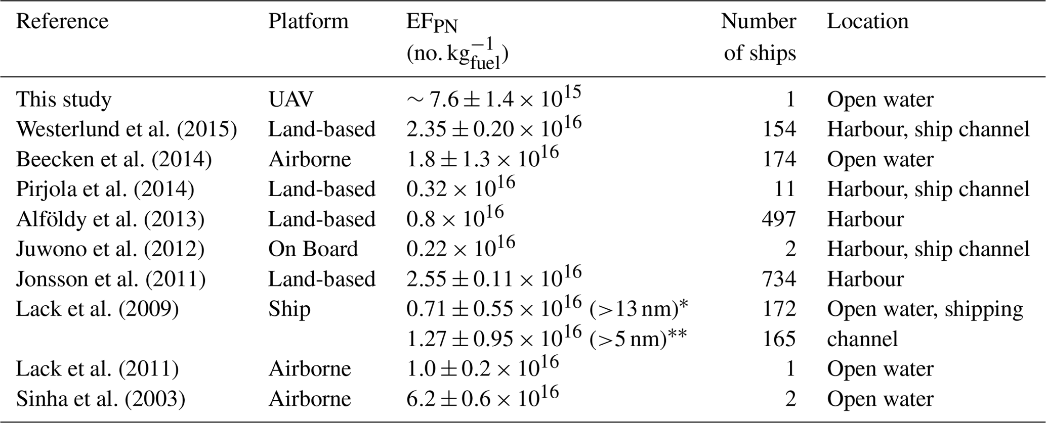
^* PN_EF for particles above 13 nm. ${}^{**}$ PN_EF for particles above 5 nm.

Download Print Version | Download XLSX

The calculated EF_PN for the Investigator was lower compared to that reported by Beecken et al. (2014) for passenger ships while accelerating ($\mathrm{0.91}\pm \mathrm{0.18}\times {\mathrm{10}}^{\mathrm{16}}$ no. kg${}_{\mathrm{fuel}}^{-\mathrm{1}}$). However, the RV Investigator measurements were undertaken whilst its engine was under 30 % load. Accelerating ships will typically be under higher engine loads and hence have a correspondingly higher EF_PN (Westerlund et al., 2015), which explains part of this discrepancy. Furthermore, the RV Investigator has high efficiency engines and utilizes ultra-low sulfur diesel fuel. Studies have shown that similar diesel engines burning fuel of this type have lower EF_PNs than the same engine with higher sulfur content diesel (Chu-Van et al., 2017). Similar quality fuels used in the ground transport industry have yielded similar values of EF_PN, ranging from 4.8×10¹⁴ (25 % engine load) to 7.2 (100 % engine load) ×10¹⁵ no. kg${}_{\mathrm{fuel}}^{-\mathrm{1}}$ (Jayaratne et al., 2009).

3.4 Instrumentation limitations

Lightweight UAVs have the potential to achieve aerial measurements at significantly less upfront and operational costs than fixed-wing and manned aerial vehicles. Lightweight UAVs can be deployed faster with limited or no required launch and landing area compared to their manned and fixed wing counterparts. Yet, their primary disadvantage, particularly in this application, is a severely limited payload weight. To overcome this limitation, this project used the lightweight and portable DISCmini and IAQ-calc sensors. However, these instruments have lower sensitivities and greater uncertainties when compared to a high accuracy CPC and CO₂ monitor for measurements, which can influence results.

The DISCmini has a manufacturer-listed measurement cut-off size of 10 nm. A previous study listed in Table 3 (Lack et al., 2009) shows that the cut-off size of instruments used to measure PNC is directly linked to the value of EF_PN, with the measured EF_PN doubling when the cut-off size is changed from 13 to 5 nm due to the large number of particles in this size range. This may have been another contributing factor to the EF_PN measured in this study being in the lower end of measured values in the literature.

The two 100 m transects were not accounted for in the final calculation of EF_PN due to their poor Gaussian curve fits. Whilst this has been attributed to the skewing of the plume at this distance, the limitations of the instrumentation could also have contributed. The lower concentrations of CO₂ at this distance result in the difference above background inside the plume being the same order of magnitude as the manufacturer-specified error margin. Hence, the variability in the plume either side of the central peak as shown in Fig. 4c could be due in part to instrumentation error.

Calibrations of sensors in this study were performed through comparison with reference instruments for ambient measurements at sea. Ideally, calibration should be performed with in-plume measurements to have the same environmental conditions and range as the real measurements. However, it was not possible to access the plume with reference instrumentation on board the ship. Whilst this study provides a successful proof of concept with consistent results over 2 days and several flights, a validation study is needed. This should include independent measurements of EF_PN using other established methodologies to ascertain more precise correction factors and uncertainties.