2.1 Measurement site

The area selected for the study is small, covering approx. 1.5 km², with a shallow, less than 150 m-deep, karst depression with a topography favourable for the formation of ground temperature inversions or cold air pools (CAPs), especially in winter. Terrain configuration of the karst depression in the north-easterly direction with a marked location of the village of Retje is shown in Fig. 1c.

Figure 1(a) Location of the study site in Europe. (b) Topographic map of the studied area with the marked fixed route and stations. (c) Profile of the terrain across the Retje karst depression with the marked village at its bottom.

Surrounded by forests in all directions and therefore influenced almost solely by 243 households with 690 residents (SiStat, 2018a, b), the site is ideal for studying impacts of residential wood burning on local air quality. Due to these characteristics, measurements at Loški Potok can be taken as representative of the atmosphere found in rural hilly regions, where wood is used as a heating fuel. For more information about the measurement site, the reader is referred to Glojek et al. (2018, 2020). In order to analyse the impact of ground temperature inversions on aerosol pollution, two temporary air quality stations with reference instruments were set up in the study area. One was placed at the bottom of the karst depression in the village of Retje (45^∘42^′34.8^′′ N 14^∘34^′53.8^′′ E; elevation 715 m a.s.l.) as a rural village site and one on top of the Tabor hill (45^∘42^′01.5^′′ N, 14^∘35^′19.7^′′ E; elevation 815 m a.s.l.) for rural background atmosphere investigation. The Tabor site was selected as a rural background location due to its position, presumably above the ground temperature inversions, with a minimal number of possible emission sources in its immediate vicinity (cemetery, rectory building, and one residential house) and with limited accessibility to vehicles yet reachable by mobile measurements, and due to the possibility of placing the air quality station there. Besides two air quality stations deployed in the study area, the 6 km-long fixed route for mobile measurements was designed along the entire hollow (Fig. 1b). The route starts in the capital of the Loški Potok municipality, i.e. in the settlement of Hrib in the south-eastern part of the karst hollow. The agglomeration is located along the regional thoroughfare and involves all the public buildings in the area (school, kindergarten, rest home, grocery store, post office, town hall, and health centre). From there the fixed mobile route leads to the top of the Tabor hill, passing the weather station in its immediate vicinity. After returning from the Tabor rural background air quality station, the route continues in the direction of the village of Retje (BR and VB). Leaving the lowest and widest parts of the hollow, the route proceeds towards the chapel of St. Florjan at the north-western-most point of the hollow. This part of the route (CR) is inaccessible to vehicles, and it is dominated by permanent pastures, including some arable land. From there the route returns to the residential area of the village of Retje, which includes the bottom part of the hollow (BV) and the slopes, facing south (VS). The mobile measurement route covers the lower part of the slopes. The fixed route around the hollow ends in the settlement of Hrib.

2.2 Aerosol measurements

In this study, the focus is on eBC mass concentrations and size-resolved measurements of particle number (PNC) and mass concentrations (PMC) of the fine particle range in winter 2017–2018. At the Retje air quality station, additional PM₁₀ mass concentrations are also available. In December 2017 and in January 2018, mobile measurements were carried out as well. The instrumentation used for the fixed stations and mobile platform is summarized in Table 1.

Table 1Description of reference and mobile instruments for eBC and PM measurements. Time is reported as local time (LT). Additional details in Glojek et al. (2018, 2020), Alas et al. (2020), and the Supplement.

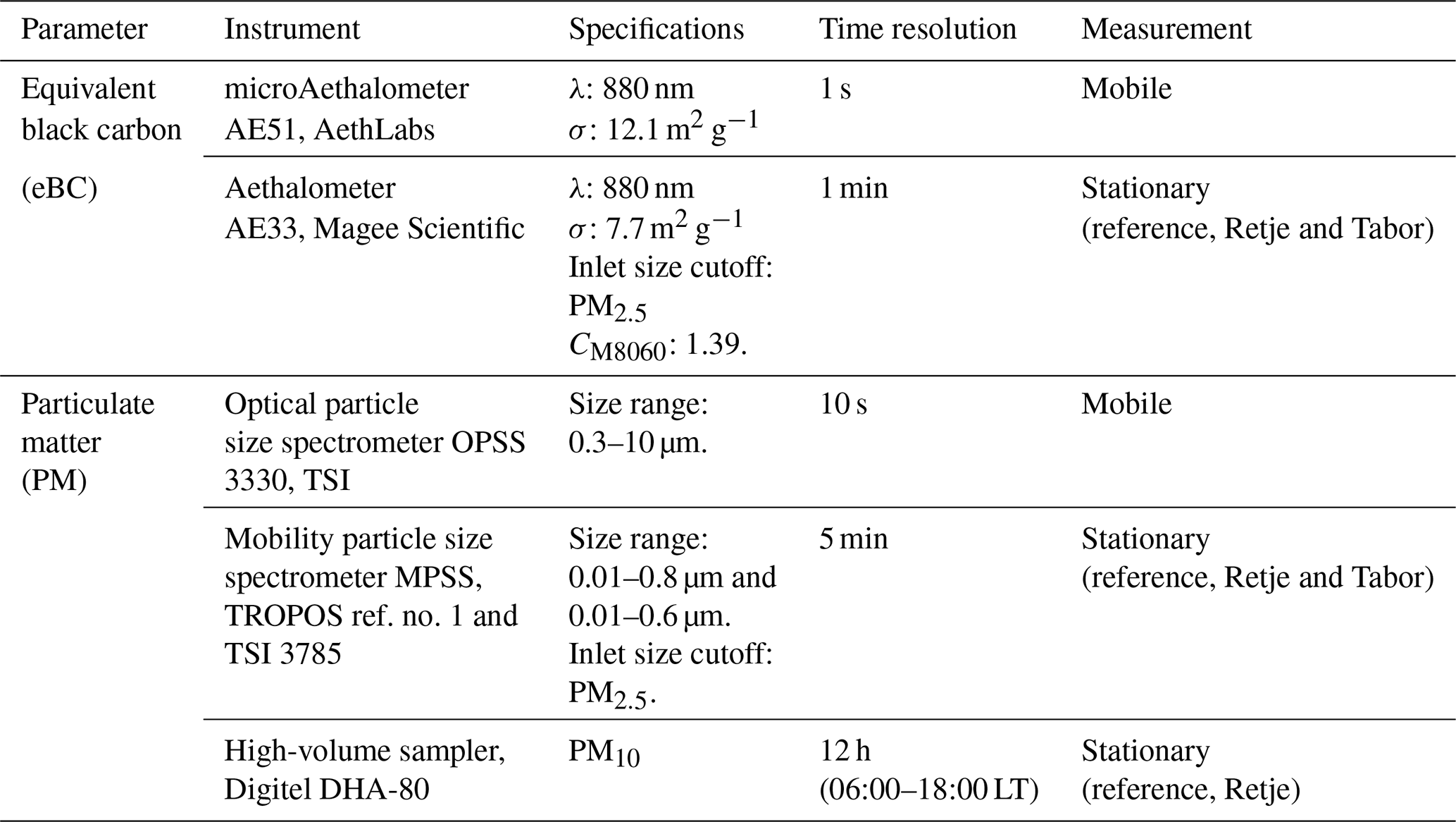
λ: wavelength; C_M8060: the correction parameter for the multiple scattering enhancement of the filter tape M8060. σ: mass absorption cross section.

Download Print Version | Download XLSX

2.2.2 Mobile eBC and PM_2.5 measurements

The mobile measurements were done using the TROPOS aerosol backpack equipped with portable instruments (Alas et al., 2019a, b, 2020). On top of the backpack, the aerosol is sampled with 1 m-long stainless steel inlet. Inside the backpack, eBC mass concentration is measured with microAethalometer AE51 (AethLab). The portable absorption photometer measures the attenuation of light at a wavelength of 880 nm through a particle-loaded T60 Teflon-coated glass fibre filter and converts it to eBC mass concentrations using σ of 12.5 m² g⁻¹ (provided by the manufacturer). Before entering the AE51, the aerosol sample passes through a silica-gel drier which dries the aerosols and dampens the effect of sudden changes in relative humidity and temperature (Cai et al., 2014; Düsing et al., 2019), which could produce false signals in the instrument. The microAethalometer was operated with a flow of 150 ml min⁻¹ and a time stamp of 1 s. In order to minimize the impacts of single events that do not represent the typical concentration profile of the area, and due to high noise of eBC mass concentrations at 1 s resolution, the data were processed to 10 s medians.

To obtain PM mass concentrations, an optical particle size spectrometer (TSI OPSS, model 3330) was used. The instrument is connected to another aerosol line inside the backpack, which is not dried. It is an optical instrument that measures the optical particle diameter according to the light scattered and the related refractive index of the calibration aerosol, typically polystyrene latex (PSL) spheres with a refractive index ($\stackrel{\mathrm{̃}}{n}$) of 1.59. However, the optical properties of ambient aerosols largely differ from the PSL, which results in wrong sizing in terms of the volume-equivalent diameter. Furthermore, the OPSS measures a PSL-equivalent size range of 0.3–10 µm, while the accumulation mode is only partially measured and the Aitken mode is not measured at all. This means that PM calculation from the OPSS PNSDs generally leads to an underestimation of the mass concentrations, which can be significant. To address this issue, the OPSS data were corrected according to the procedure briefly described in the latter part of this section, which follows the methodology presented in Alas et al. (2019a). During the Loški Potok campaign, the OPSS had a flow of 1 L min⁻¹ and a 10 s time resolution. The position of the mobile measurements was obtained by a GPS device placed on top of the inlet. All instruments together with the GPS unit were synchronized and controlled by a microcomputer where the data were also logged.

Simultaneous mobile measurements with two instrumented backpacks were carried out three times a day along a fixed route in the Retje karst depression. The run in the morning lasted from 06:30 to 09:00, at noon from 12:00 to 14:00, and in the evening from 17:00 to 19:00 LT. To obtain representative information, daily measurements along the depression were conducted 107 times, totalling 642 km. Results of the convergence analysis (see Alas et al., 2020, and the references therein for the assessment process) for all data points in the village of Retje and at the Tabor hill are depicted in Fig. S12. The number of runs when the cumulative median concentrations of randomly selected runs deviate less than 50 % from the median of all the runs at the given location was selected for a threshold. According to visual analysis, the data converged more quickly for the Tabor hill compared to the village of Retje. Thus, the minimum number of runs required to obtain a representative image of the air quality on the Tabor hill is 46 for eBC and 52 for PM_2.5, whereas for the village of Retje it is 65 for eBC and 58 for PM_2.5.

Table 2Air quality measurement stations with the “reference” aerosol instruments at the study site.

Download Print Version | Download XLSX

The route (see Fig. 1b) led past fixed stations with the following reference instruments: the AE33 Aethalometer and the MPSS (Table 2). During each run the carriers of the backpacks intercompared the mobile AE51s with the AE33 Aethalometers and the OPSSs 3330 with the MPSSs. Intercomparison at the Retje site (the rural village station) lasted 20 min and, at the Tabor site (the rural background site), 10 min. The methodology used to ensure high-quality mobile measurements of eBC and PM mass concentrations is provided in Alas et al. (2019a).

In order to obtain accurate eBC mass concentrations, mobile filter photometers were corrected for the filter-loading effect (FLE). The correction algorithm presented by Virkkula et al. (2007) was used, with a loading parameter (k) of 0.005 for the AE51 microAethalometers based on Drinovec et al. (2017). Besides diesel-dominated aerosols, the selected value of k is representative of freshly emitted particles from wood burning as well. Detection of the filter-loading effect, correction, and correlation between the AE51 microAethalometers against reference instruments (the AE33 Aethalometers) used in the Loški Potok campaign is published in Alas et al. (2020).

As previously stated, PM_2.5 mass concentrations were derived from the OPSS measurements that were corrected by the aerosol-type-dependent complex refractive index ($\stackrel{\mathrm{̃}}{n}$) and unique fine-mode volume correction factors (CFs_f, vol). The real part (${\stackrel{\mathrm{̃}}{n}}_{\mathrm{re}}$) of the OPSS $\stackrel{\mathrm{̃}}{n}$ was adjusted to 1.52 and the imaginary part (${\stackrel{\mathrm{̃}}{n}}_{\mathrm{im}}$) to i0.02 for all size bins. Both values are typical for rural, residential areas containing absorbing aerosols (Ebert et al., 2004; Lu et al., 2015). However, applying one corrected $\stackrel{\mathrm{̃}}{n}$ for particles in the range 0.3–0.8 µm, as well as for the particles larger than 0.8 µm, could lead to high uncertainties due to unknown particle shape and light-absorbing particle composition in the supermicrometre range. After the $\stackrel{\mathrm{̃}}{n}$ correction had been applied to the OPSS PNSD using Mie theory, the optical diameters were converted to geometric mean volume-equivalent diameters for the submicrometre size range (the correction of the data is illustrated in Figs. S7, S8, and S9). The CF_f, vol corrects the OPSS constraint of measuring only a fraction of the fine-mode particles (from 0.3 to 10 µm). Therefore, CFs_f, vol were calculated as a ratio between the fine mode of the OPSS (from 0.4 to 0.8 µm) with the fine mode of the MPSS (from 0.001 to 0.8 µm) during each intercomparison period, since the variability of particle volume size distributions (PVSDs) requires the use of a unique CF_f, vol for each individual run (Alas et al., 2019a). As there are no significant differences in aerosol sources along the hollow (see Glojek et al., 2018) and due to instrument failures at the second measurement location, data points of the whole selected route were corrected with the correction factors derived at the Retje rural village station. The relevance of the use of correction factors obtained at a single measurement site (Retje) for the entire route was confirmed by the comparison of the PVSDs measured by the MPSS at the Tabor rural background station. That is, PVSDs at both measurement sites peaked around 0.3 µm (see Fig. S8). Once all the corrections were applied for each run, PM₁ mass concentrations were calculated. Since the organic aerosols prevail in the studied area, a particle density of 1.5 g cm⁻³ (Turpin and Lim, 2001) was used for the calculation. The absolute value of PM₁ was added to the absolute value of PM_1−2.5 to obtain PM_2.5 mass concentrations. Corrected PM₁ mass concentrations of the OPSS are comparable to the reference MPSS. Correlation between median PM₁ mass concentrations obtained from the OPSS and MPSS during each intercomparison time is high, with R²>0.8 and a slope of 1.12. Additionally, PM₁ mass concentrations derived from the MPSS measurements were compared to the 12 h PM₁₀ data, measured by the High-Volume Sampler Digitel DHA-80. These two parameters correlate well too, with R²=1 and a slope of 0.9 (Fig. S7). The relationship shows that most of the mass concentration of PM₁₀ is already found in PM₁. Despite considerably improved calculated PM_2.5 mass concentration values of the OPSS after applied corrections, some uncertainties remain, primarily due to the particle non-sphericity, assumed particle density, and the use of the same time-dependent correction factors for the whole route. With an increase in particle size, the shape of the particles becomes even more non-spherical, and thus the refractive index correction based on Mie theory, assuming spherical particles, is not possible. Due to this high uncertainty, PM₁₀ mass concentrations from the OPSS data were not calculated for this study.

2.3 Meteorological parameters

Hourly and daily averages of meteorological parameters recorded from air quality stations in Retje and at Tabor (ambient temperature, pressure, and relative humidity) and from the weather station of the non-governmental Society for Weather and Climate Research (Društvo za raziskovanje vremena in Podnebja, 45^∘42^′4^′′ N 14^∘35^′27^′′ E, elevation 775 m a.s.l.) for ambient temperature, pressure, relative humidity, wind speed and direction, and the sum of precipitation were computed. The location of the weather station is marked with the black cross (Hrib in Fig. 1b). To determine temperature inversion episodes, mobile temperature measurements with a temperature sensor (DS1922L iButton, Maxim Integrated) were considered as well. Besides the observed meteorological variables, heating degree days (HDDs) were determined from the daily mean temperatures at the stations. The index was calculated according to Eurostat (2019) as well as ARSO (2021) methodology. The former uses a daily threshold value, defined as the lowest daily mean air temperature not leading to indoor heating, of 15 ^∘C and the latter 12 ^∘C.

2.3.1 Detection and selection of temperature inversion periods

Temperature inversion periods in the selected karst depression were detected by analysing the calculated potential temperature gradient, obtained from ground-based observations of temperatures at different elevations and the mobile temperature measurements along the hollow. The ratio of temperature differences between stations at different heights is a good indicator of the stability of the boundary layer during temperature inversions as shown in, for instance, Petkovšek (1979), Whiteman et al. (1999, 2014), Pandolfi et al. (2014), Holmes et al. (2015), and Largeron and Staquet (2016). In our study potential temperature differences between the Retje station at the bottom of the karst depression, the Hrib station on the slope, and the Tabor station on top of the hill were calculated ($\mathrm{\Delta }\mathit{\theta }/\mathrm{\Delta }Z$). Mobile measurements of potential temperatures in December along the Retje karst depression were used as the Supplement to determine atmospheric conditions during the runs. If potential temperatures during mobile measurements along the karst depression were increasing with altitude (positive gradient), the runs were classified as runs during the temperature inversions. However, if potential temperatures were decreasing (negative gradient), the runs were classified as runs with an unstable atmosphere. To conform to the defined atmospheric conditions, other meteorological variables were considered as well. The number of classified runs during temperature inversion and during an unstable atmosphere is represented in Table 3.

Table 3Number of runs in winter 2017–2018 classified as runs during temperature inversion and runs during unstable atmosphere. The number of runs with strong temperature inversion is shown in brackets.

Download Print Version | Download XLSX

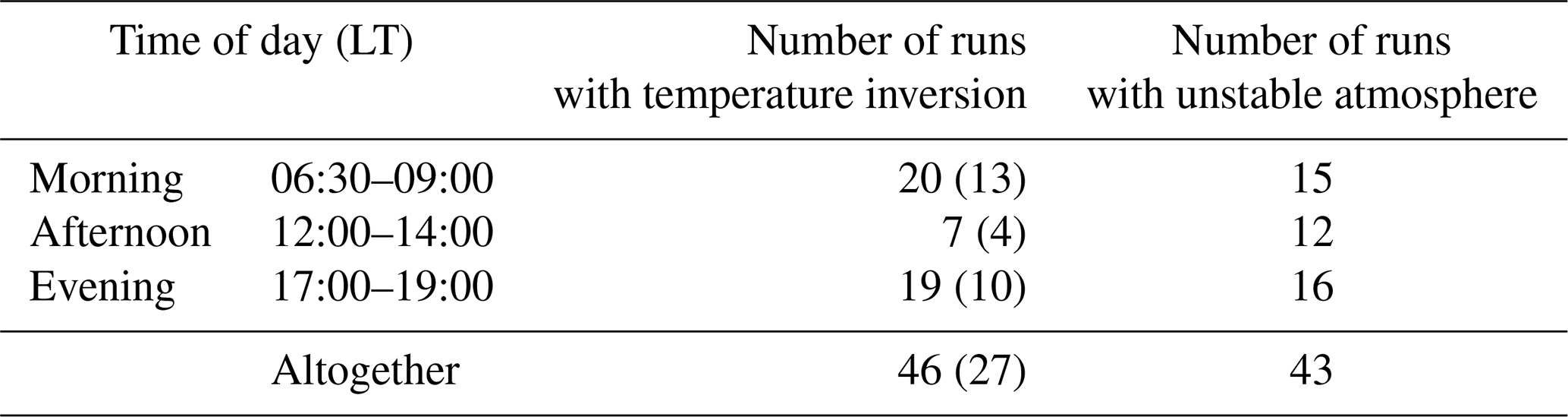
Out of the total of 107 runs performed along the hollow, 98 were valid, i.e. without measurement failures (e.g. leak in the system, wrong GPS route tracking, full filter), and classified according to the meteorological conditions. Forty-six runs were classified as runs during temperature inversion, of which 27 had strong temperature inversion (the numbers indicated in brackets). The criteria for further separation of the temperature inversions are determined by the potential temperature gradient above 1 K (100 m⁻¹) and by the change in the weather regime during the run. Thus, a run with strong temperature inversion stands for the run with a potential temperature gradient above 1 K (100 m⁻¹) during the whole run with no weather changes or intensive mixing of the atmosphere during the run. Forty-three runs had a negative potential temperature gradient during the whole run and were therefore classified as runs with an unstable atmosphere. During nine of the runs atmospheric conditions changed from stable to unstable or vice versa and thus were not taken into account in the analysis according to meteorological conditions.

2.4 Spatial and statistical analysis

Concerning the second goal, mobile measurements were spatially averaged according to the method described in Alas et al. (2019a, b). Firstly, a pre-determined route with 10 m equidistant points in QGIS 2.18.22 was created. These points were used as centre points for spatial aggregation performed in the R programming language. Prior to spatial aggregation, mobile runs were separated into two groups according to atmospheric conditions: runs occurring during temperature inversions and runs with an unstable atmosphere (for the classification of runs with respect to meteorological conditions, see Sect. 3.3.1). Subsequently, the median of all data points in a radius of 10 m around each centre point was calculated. Results are moving circular medians of eBC and PM_2.5 mass concentrations along the route calculated separately for all the runs during strong temperature inversions (27) and for all the runs during an unstable atmosphere (43). In addition, average ambient ratios of eBC to PM_2.5 for the whole hollow were calculated.

For the goal of establishing an association between aerosol pollution and meteorology, correlation analyses between meteorological variables with eBC and PM mass concentrations for the whole measurement period and for the selected days with temperature inversion (temperature inversion days) and days with an unstable atmosphere (non-inversion days) was performed. An ordinary least squares (OLS) linear regression was applied using the Python programming language with the “scipy” module.

Finally, we investigated the number of people living in rural hilly and mountainous areas across Europe. An enquiry analysis of the European Digital Elevation Model of 25 × 25 m (Copernicus Land Monitoring Service, 2007) was performed. The analysis was conducted for the European Mountain Areas (2008), excluding the Turkish peninsula and islands except those that are part of the mountain range (e.g. Sicily) and Iceland. Relief depressions were identified with the TPI-based Landform tool in the SAGA GIS 2.3.2 software environment. Landform classes such as drainages, valleys, and plains bigger than 0.4 km² were selected for further analysis. As we were interested in populated rural relief hollows, uninhabited and urban areas were eliminated with the help of a population density grid of 1 km² (GEOSTAT, 2011) and with the spatial classification “Degree of urbanisation” (DEGURBA, 2016). Data manipulation was done using Python and ArcGIS 10.8.1. The results are shown in the Supplement (Fig. S15).

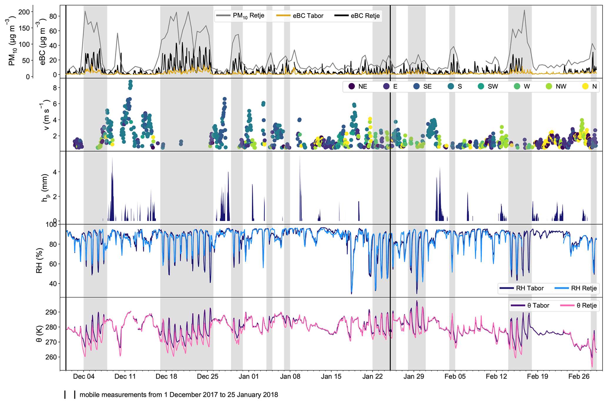
Figure 2Time series of meteorological and air quality data for the winter period (1 December 2017–1 March 2018): the 12 h PM₁₀ mass concentrations at Retje, the hourly mean eBC mass concentrations at Retje and Tabor, wind speed (v) and direction at Hrib, precipitation (h_p) at Hrib, and relative humidity (RH) and potential temperature (θ) at Retje and Tabor. The shaded areas represent temperature inversion periods.

Download

3.1 Meteorological conditions, PM₁₀, and eBC mass concentrations

Twelve-hour PM₁₀ and hourly averages of eBC mass concentrations and meteorological conditions during winter (1 December 2017–1 March 2018) and during the mobile measurement period (1 December 2017–25 January 2018) are illustrated in Fig. 2. Shaded areas represent selected temperature inversion periods, when the potential temperature at the Retje station at 715 m a.s.l. (pink line) was lower than the potential temperature at the top of the Tabor hill at 815 m a.s.l. (purple line). As described in the method section (2.3) and in Glojek et al. (2018), wind data were collected at Hrib at 775 m a.s.l. The location of the wind measurements out of the hollow is not the most representative of the wind characteristics in the very basin. Thus, wind speeds in the hollow are expected to be lower due to topography, which prevents effective ventilation.

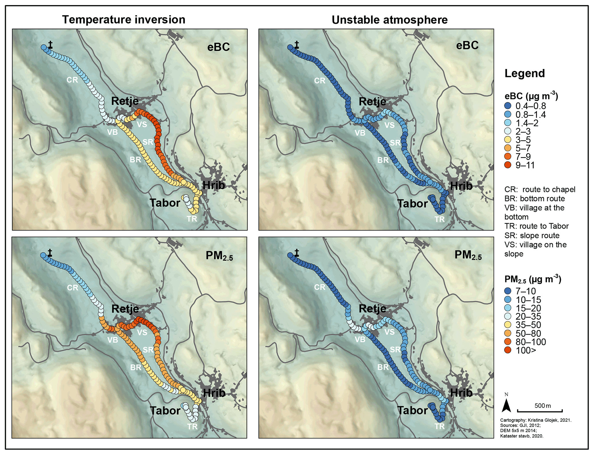
Figure 3Spatial distribution of eBC (upper part) and PM_2.5 (lower part) mass concentrations during temperature inversions (left-hand side) and during unstable atmosphere (right-hand side) along Retje karst hollow. The spatial average of pollutant levels or all selected runs is presented.

Rapidly changing meteorological conditions and pollutant mass concentrations were observed during the whole winter period 2017–2018. eBC mass concentrations at the bottom of the hollow in the village of Retje (black line) were consistently higher than at the rural background station on top of the Tabor hill (yellow line). It was at the Tabor station where a smaller range of eBC mass concentration levels was recorded overtime as well. Mean hourly eBC concentrations at Tabor ranged from a few hundred ng m⁻³ to 20 µg m⁻³, while eBC concentrations at Retje were in the range from 0.9 µg m⁻³ (25th percentile) to above 40 µg m⁻³. PM₁₀ levels varied between below 10 and up to 205 µg m⁻³ at the village of Retje (grey line).

Intensity of sources and meteorological variability are followed by changes in pollutant concentrations. The highest eBC mass concentrations at both measurement sites were observed during two longer periods of a stable atmosphere in December 2017. Similar results were found for PM₁₀ as well. There was also a third distinct increase in pollution levels at Retje during the longest temperature inversion period in February. However, the eBC data for this period are partly missing. The first period lasted from 4 to 8 December, the second period from 17 to 25 December, and the third period from 14 to 18 February. The second period in December presents the longest period with temperature inversion of the whole campaign. All of these periods were characterized by anticyclonic weather with no or weak, lower than 0.7 m s⁻¹ wind speeds, the absence of precipitation, and low temperatures at the bottom of the hollow, reaching a trough of −18.4 ^∘C on 15 February at the Retje station. Due to lower temperatures at the bottom of the hollow than on top of the hill, the relative humidity in the hollow was higher than on the Tabor hill. Morning and evening temperatures in the hollow dropped regularly below the dew point during temperature inversions, forming radiation fog. Regular diurnal eBC, temperature, and relative humidity oscillations could be seen during temperature inversions. The valley floor was covered with snow during all three temperature inversion episodes. The period between the first and second longer temperature inversions in December, i.e. from 8 to 16 December, was characterized by an intense frontal activity with strong, from 2 m s⁻¹ (25th percentile) to 4 m s⁻¹ (75th percentile) southerly to south-easterly winds with gusts above 9 m s⁻¹ and high snow precipitation with 61 cm of new snow recorded. After 10 December there was a strong thaw with warm air masses. After the second temperature inversion period in December, the temperatures rose again and stayed above the long-term average for the whole month of January and at the beginning of February (see Glojek et al., 2018). Precipitation in the form of rain was above the long-term average in comparison to the usual amount of rainfall in January (Cegnar and Knez, 2018). Out of 14 precipitation days in January, only 4 d had snow. In January and at the beginning of February, periods with temperature inversions were shorter compared to December, lasting no longer than 4 d, with higher temperatures and lower relative humidity, respectively, 2.5 ^∘C higher and 7.6 % lower mean values at all the stations. Moreover, the PM₁₀ and eBC mass concentration levels during January and February temperature inversions were lower compared to temperature inversions in December, except from 14 to 18 February, when PM₁₀ mass concentrations reached maximum levels. In Retje, mean PM₁₀ and eBC levels were, on average, more than 2 times lower, with means of 133.5 ± 42.3 and 12.9 ± 10.7 µg m⁻³, respectively, for December inversions and means of 56.2 ± 19.9 of PM₁₀ and 6.3 ± 6.7 µg m⁻³ of eBC for inversions in January and February. Due to missing data, the longest temperature inversion episode in February was not included in the calculation. At Tabor the difference between a mean value of 3.6 ± 3.3 µg m⁻³ for December inversions and a mean of 2.3 ± 2.7 µg m⁻³ for inversions in January and February was 1.3 µg m⁻³ of eBC. In February temperatures dropped, especially in the last days of the month, when temperature in Retje dropped below −24.7 ^∘C, reaching minimum temperatures for the winter of 2017–2018. Cold and moist easterly and north-easterly winds prevailed over the area, bringing snow precipitation. In February there were more than 19 d with precipitation, including 17 d of snowfall and 26 d of snow cover. Cloudy weather prevailed during the whole month. Temperature inversions occurred mainly within the first and second thirds of February.

Table 4Summary of eBC and PM_2.5 mass concentrations measured along the route of the Retje karst depression. Mean with standard deviation (AM ± SD), median (MED), and average eBC $/$ PM_2.5 ratio of the whole route during temperature inversions and during unstable atmosphere shown for all the runs (all) and separately according to different run times. MIN and MAX represent the value and location of the pollutant minimum and maximum along the route.

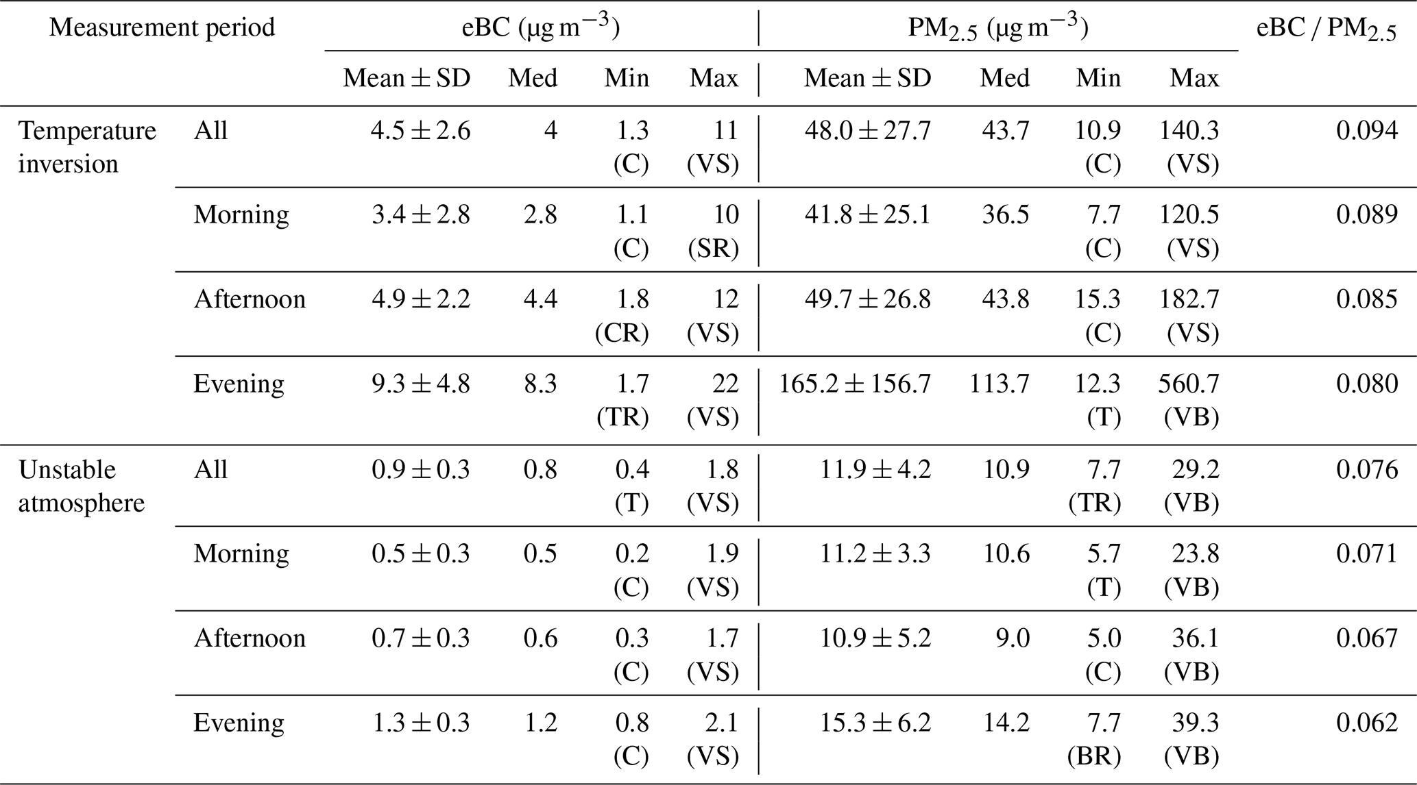
C and CR: chapel and route to chapel. BR: bottom route. VB: village at the bottom. T and TR: Tabor and route to Tabor. SR: slope route. VS: village on the slope.

Download Print Version | Download XLSX

3.2 Spatiotemporal variability of eBC and PM_2.5 during temperature inversion and during unstable atmosphere

As already seen in time series of eBC and PM₁₀ mass concentrations at the stations in Fig. 2, concentration levels vary in time as the conditions in atmosphere change. The highest eBC mass concentrations were observed during temperature inversions, while the lowest values were detected during the unstable atmosphere with the negative vertical temperature gradient. Figure 3 (upper part) shows the spatial distribution of eBC and Fig. 3 (lower part) illustrates PM_2.5 mass concentrations during different exemplary meteorological conditions along the hollow. The spatial average of pollutant levels for all selected runs is presented.

Figure 4Variability of eBC (top panels) and PM_2.5 (bottom panels) mass concentrations during morning (06:30–08:30 LT, red line), afternoon (12:00–14:00 LT, yellow line), and evening (17:00–19:00 LT, purple line) winter-time temperature inversion along different parts of the fixed route in the Retje hollow.

Download

During winter temperature inversions eBC and PM_2.5 mass concentration levels build up in the whole hollow with mean values of 4.5 ± 2.6 µg m⁻³ of eBC and 48.0 ± 27.7 µg m⁻³ of PM_2.5. However, considerable differences are observed among different positions in the relief depression. The highest pollutant mass concentrations are observed at the south-eastern end of the hollow, in the village of Retje, near the air quality station (VS) and along the first part of the slope road (SR) that connects the village of Retje with the settlement of Hrib. The PM_2.5 mass concentrations are highest close to the agglomeration of Retje (Fig. 3 on the lower left-hand side), whereas the eBC mass concentrations are highest along the slope road (Fig. 3 on the upper left-hand side). Mass concentrations in this area reach 11 µg m⁻³ of eBC and 140.3 µg m⁻³ of PM_2.5 on average. In contrast to pollutant maxima, the lowest eBC and PM_2.5 mass concentrations were measured out of the village at the chapel of Florjan in the north-western-most part of the hollow. Mean eBC mass concentrations of 1.3 µg m⁻³ and mean PM_2.5 of 10.9 µg m⁻³ were 9 to 13 times lower than at the village of Retje. On the Tabor hill at the other, south-easterly end of the hollow above the settlement of Hrib, mean values of eBC and PM_2.5 were 2 and 17 µg m⁻³, respectively. Mean eBC mass concentrations of 4 µg m⁻³ were observed along the route to the village of Retje (BR). Levels of PM_2.5 were increasing from 32 to 60 µg m⁻³ along the route towards the village (BR), which lies at a lower altitude. The eBC trend, however, depends on the time of the day (Fig. 4). In the morning, from 06:30 to 09:00, eBC levels with a mean value of 3 µg m⁻³ remain constant along the whole bottom route (BR), whereas around noon and in the early evening, eBC mass concentrations change along the route. As seen with the PM_2.5 levels, early evening eBC mass concentrations increase from 6.6 to 11.6 µg m⁻³ in the direction of the village of Retje as well. Conversely, around noon, eBC mass concentrations are higher in the part of the route leading to the settlement of Hrib (SR), which is at a higher altitude, increasing from 4.0 to 7.5 µg m⁻³.

During an unstable atmosphere (right-hand side of Fig. 3), mean mass concentrations of eBC and PM_2.5 in the entire hollow do not reach 1 µgm⁻³ of eBC and 12 µg m⁻³ of PM_2.5. Nonetheless, increased eBC and PM_2.5 mass concentrations in the village of Retje are observed, reaching 1.8 µg m⁻³ of eBC and 29.2 µg m⁻³ of PM_2.5 on average. A slight increase in mass concentrations is seen near the settlement of Hrib as well, with mean eBC of 0.8 µg m⁻³ and mean PM_2.5 of 15 µg m⁻³. The ratios of eBC $/$ PM_2.5 during the winter 2017–2018 campaign observed in the model region Loški Potok ranged from 0.062 to 0.094. The relationship between eBC and PM_2.5 mass concentrations per coded locations along the route is shown in Fig. S11. Correlation is good for all locations (R²>0.6 or R²=0.6), especially for non-traffic ones (R²>85). The eBC mass fraction in PM_2.5 is higher at Tabor (T and TR) and Hrib (H) compared to locations in the hollow.

A deeper analysis of the pollutants' spatial distributions during temperature inversions is shown in Fig. 4. The determined line segments along the fixed route inside the Retje hollow are listed and described in Table 4, with their spatial locations marked in Fig. 5. Here, the goal was to show horizontal variability of eBC and PM_2.5 along the hollow with respect to different times of the day. To this end, line segments at similar relative heights were selected (a maximum difference of 30 m per route segment; see Table 5).

Table 5List and description of the different route segments along the Retje hollow.

Download Print Version | Download XLSX

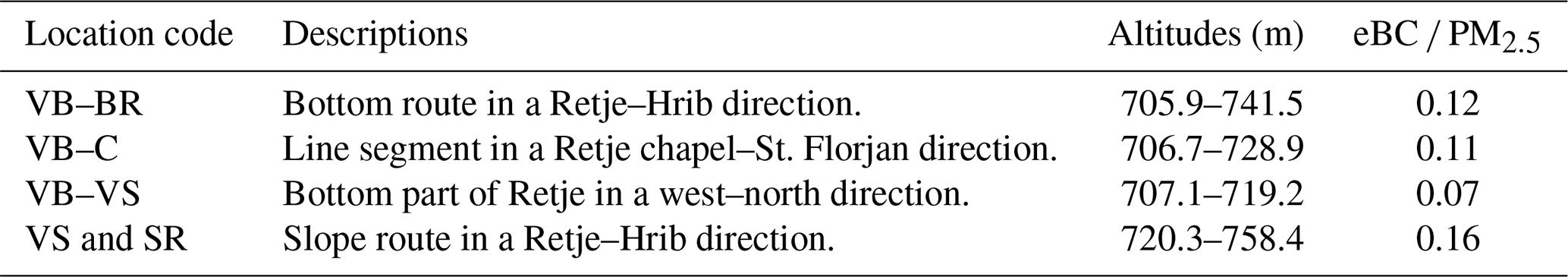
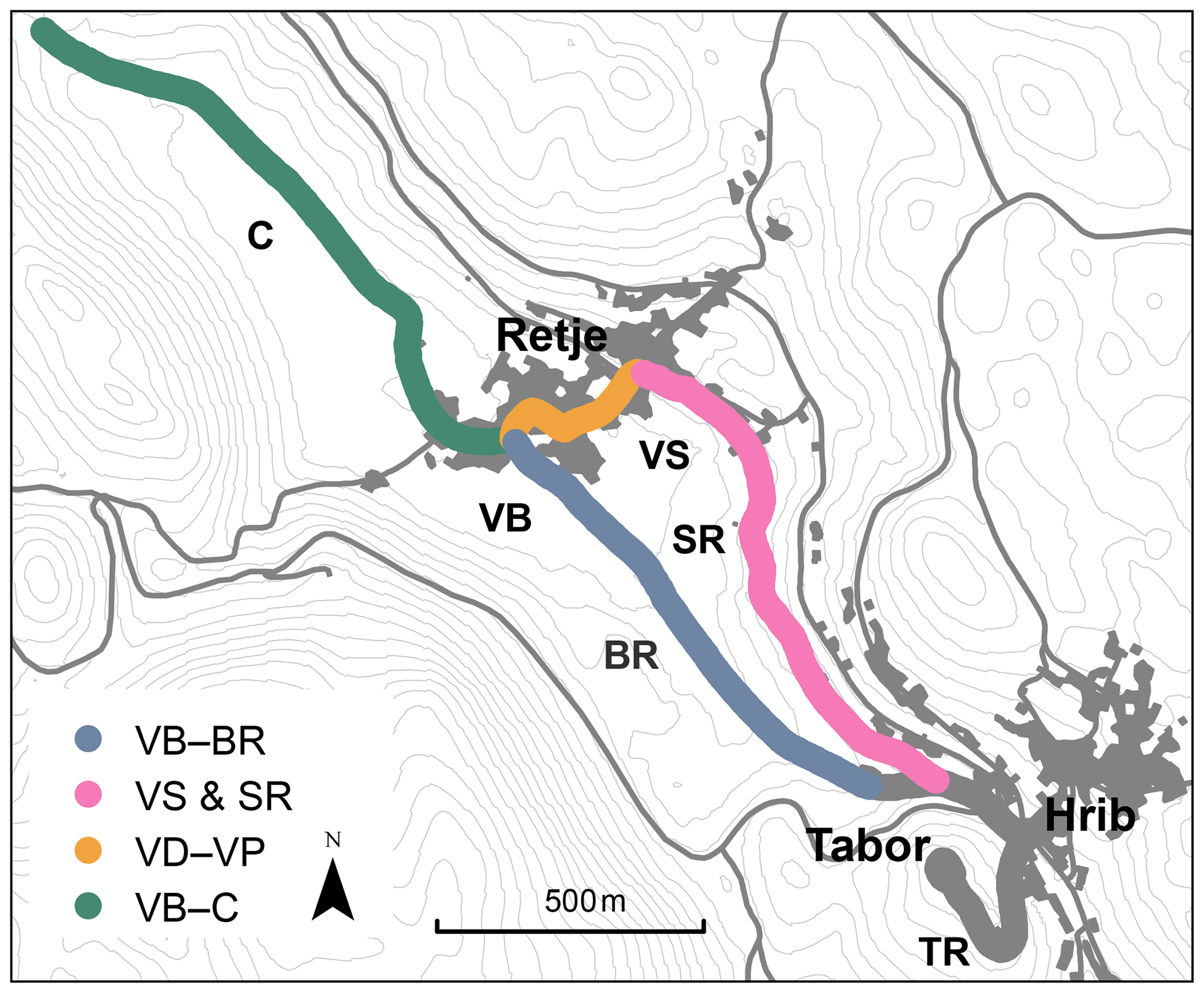
Figure 5The location codes assigned to the line segments of the fixed route.

The eBC and PM_2.5 mass concentration variability trend differs throughout the route, and it is day-time-dependent as well. That is, mass concentrations of both pollutants are 2 to 4 times higher during evening temperature inversions as compared to inversions in the morning and in the afternoon. This applies to all locations inside the hollow. However, the difference between the run times is highest in the village of Retje, with up to 5 and 7 times higher evening eBC and PM_2.5 levels, respectively.

Unlike the PM_2.5, the eBC trend along the line segment VB–BR depends on the time of the day. In the morning, from 06:30 to 09:00 LT, eBC levels with a mean value of 3 µg m⁻³ remain constant along the whole BR, whereas around noon and in the early evening, eBC mass concentrations vary. As seen with the PM_2.5 levels, early evening eBC mass concentrations increase from 6.6 to 11.6 µg m⁻³ towards the village of Retje. In the other direction, from the village of Retje to the St. Florjan chapel (VB–C), levels of both pollutants decrease, with the highest drop observed during evening temperature inversions, particularly in PM_2.5.

Horizontal gradients of the pollutants' mass concentrations differ most at the village of Retje located at the bottom of the hollow (VB–VS) and at the slope street in the direction from the village of Retje towards the settlement of Hrib (VS and SR). This relates to morning and evening temperature inversion runs, while for the afternoon runs the variability of the pollutants is similar. In the morning and in the evening, PM_2.5 mass concentrations over the whole village at the bottom of the Retje hollow are elevated and steeply decline further away from the village, especially in the evening. In the afternoon, however, greater mass concentrations were measured along the village on the slope (VS). This is seen in Fig. 4, line segment VB–VS, as a sharp increase in PM_2.5 mass concentrations at a distance of 200 m away from the starting point of the route segment. The decrease in eBC along the slope road (VS and PC) from the village of Retje towards Hrib is smaller than that of PM_2.5. Moreover, during morning runs, eBC mass concentrations in the middle of the road segment increase, i.e. from 4.4 to 9.2 µg m⁻³.

3.3 Mixing height during temperature inversions

The MH was determined for the selected temperature inversion events, based on eBC vertical profiles collected with mobile measurements described under Sect. 2.3.2. Despite the method shortcomings, applied data quality measures ensure that the requirements of the study's purpose are met (see the following Sect. 3.3.1). The lowest point in the hollow captured by mobile measurements is at 705.9 m a.s.l. (the lowest elevation of the hollow is 700 m), while the highest point is at the top of the Tabor hill at 815 m a.s.l. (the highest point of the hollow's rim is at about 900 m a.s.l.).

Figure 6Mean vertical eBC and PM_2.5 profiles with standard deviation (shaded area) during morning (06:30–08:30 LT, red line), afternoon (12:00–14:00 LT, yellow line), and evening (17:00–19:00 LT, purple line) winter-time temperature inversions over the Retje hollow.

Download

In Fig. 6 the 5 m-averaged vertical profiles of eBC and PM_2.5 mass concentrations are depicted for all morning (06:30–09:00 LT), afternoon (12:00–14:00 LT), and evening (17:00–19:00 LT) runs during temperature inversions. Particle accumulation in the mixing layer results in a strong concentration gradient indicating the MH. From eBC vertical profiles the mixing layer boundary is clearly visible as a sudden and significant decrease in eBC mass concentrations (all vertical profiles during temperature inversions obtained with mobile runs are illustrated in the Supplement, Fig. S13). On average, during strong winter temperature inversion events (46 runs), the MH in the hollow is 58 ± 15 m. For temperature inversions with a stronger temperature gradient of about 4.7±1.7 K (100 m)⁻¹, prevailing in December, the MH is on average 6 m higher (61 ± 15 m) than during temperature inversions, with a weaker temperature gradient of 2.5 ± 2.1 K (100 m)⁻¹ (55 ± 12 m).

Table 6Calculated mean MH during all morning, afternoon, and evening runs with ground temperature inversions, derived from eBC vertical mass concentration profiles (N=46). The MHs are rounded to 5 m.

Download Print Version | Download XLSX

During stagnant atmospheric conditions a slight evolution in day-time MH is observed (Table 6 and Fig. 7). The highest MH is detected during morning and afternoon runs, with a MH of about 60 m, whereas the lowest MH is in the early evening, with a mean MH of 55 m. The highest variability of the mixing boundary layer height is observed around noon-time, with the MH in the range between 40 and 105 m. As seen in Fig. 7, most of the points are positioned at 70 m MH, especially during morning runs. This corresponds to the height of the drainage area at the south-eastern part of the hollow influenced by locally induced flows. Moreover, there are fewer emission sources above this height than in the lower parts of the hollow.

The MH increases during stronger temperature inversions in the morning and decreases during weaker temperature inversions at noon. Nonetheless, this information must be treated with caution since only seven afternoon runs were conducted, during which temperature inversion occurred.

Figure 7Mixing height (MH) during morning (06:30–08:30 LT), afternoon (12:00–14:00 LT), and evening (17:00–19:00 LT) runs with temperature inversion. Statistics for every run time in a day are represented by a boxplot (cross: mean, horizontal line: median, box: 25th–75th percentile, whiskers: 5th–95th percentiles).

Download

eBC mass concentrations within the MH (average of 8.2 µg m⁻³) are almost 3 times higher than just above the MH in the free atmosphere (average of 3.2 µg m⁻³). On average, the free atmosphere represents 17 % of the total concentrations within the mixing height and 14 % of the total concentrations in the whole measured vertical profile. The lowest eBC mass concentrations during temperature inversions were measured during morning runs. The mean eBC mass concentrations detected in the whole vertical profile were 4.0 ± 4.2 µg m⁻³, within MH 5.0±4.5 µg m⁻³, and above MH 1.7 ± 1.6 µg m⁻³. Early evening runs are characterized by the highest eBC mass concentrations, with mean eBC levels of 12.3 ± 8.9 µg m⁻³ within the mixing height, 4.2 ± 3.4 µg m⁻³ above MH, and 9.8 ± 8.5 µg m⁻³ in the whole vertical profile. During afternoon runs the difference between mass concentrations within the MH and just above the MH was 2 times smaller than during morning and evening runs. The mean eBC value within the MH was 6.9 ± 5.0 µg m⁻³ compared to 5.1 ± 3.7 µg m⁻³ of eBC detected just above the MH. On average, eBC mass concentrations in the free atmosphere represented 32 % of the total eBC mass concentrations within the mixing height.

Besides the strong eBC mass concentration gradient, representing the border of the MH, two other layers of high eBC mass concentrations are seen in most of the eBC height profiles (Fig. S13). As seen on the spatial maps (Fig. 3), the first increase in eBC as well as PM_2.5 levels arises close to the hollow's floor and coincides with the elevation of the village of Retje at around 710 m a.s.l. (VB). The second increase occurs on the populated slope (SR), facing south, between 725 m and 745 m a.s.l. In the early evening the highest eBC mass concentrations are observed near the bottom of the hollow (VB), reaching 22 µg m⁻³. At that time PM_2.5 mass concentrations at the village of Retje reach maximum mass concentrations as well, reaching 560.7 µg m⁻³.

3.4 Association between meteorological variables with eBC and PM at the fixed stations

Correlation analysis between hourly and daily meteorological variables and eBC mass concentrations at both air quality stations revealed a statistically significant correlation between eBC levels and temperature, HDD, ambient pressure, wind speed, and the potential temperature gradient. No statistically significant association was found in the following meteorological variables: wind direction (N=73) and daily sum of precipitation (N=38). The conditions for correlation analysis between MH and pollution levels or any other meteorological parameter have not been fulfilled, as the determination of MH was done only for the runs during temperature inversions (N=47) with a limited height range between 25 and 105 m, mostly from 40 to 75 m. A stronger correlation between most of the variables is found at the Retje site, located in the hollow, than at the Tabor rural background station, positioned on top of the hill. The only exceptions were the wind speed measurements performed at the Hrib meteorological station, positioned outside the hollow. At the village station correlation analysis with 24 h PM₁₀ samples was conducted as well. Very similar correlation coefficients were obtained as for 24 h average eBC mass concentrations and are presented in Table 7.

Table 7Regression results for the relation between meteorological conditions, eBC and PM₁₀ mass concentrations (µg m⁻³) (24 h averages) in winter 2017–2018, and selected days with temperature inversion and unstable atmosphere (in brackets) at both air quality stations – the Retje rural village station (eBC and PM₁₀) and the Tabor rural background station (eBC). In the last column the means of meteorological parameters with SD are given.

^* Data from the Hrib station (775 m a.s.l.).

Download Print Version | Download XLSX

At both sites the relation between the temperature and eBC mass concentrations is confirmed at p<0.001. On the other hand, only a very weak correlation (R²=0.2, slope $=-\mathrm{0.1}$) is found at the Tabor rural background station and a little bit higher at the Retje station, with R² amounting to around 0.4. The same influence is also observed for PM_10. The relationship is negative, meaning that eBC and PM₁₀ mass concentrations decrease with higher temperatures, on average by −0.51 and 5.79 µg m⁻³, respectively. The results, however, are not very reliable as the correlation is moderate. The same relationship is found for HDD (Eurostat, 2019; ARSO, 2021). According to the HDD index, there was a need for indoor heating on all winter days.

Relation analysis of wind speeds and eBC was performed, which considered only days with no precipitation and wind speeds higher than 0.09 m s⁻¹. The location of the wind measurements is not representative of the conditions on the floor of the hollow. Therefore, correlation analysis is adequate only for the station on the Tabor hill. However, merely a moderate correlation was found for the winter days. The relationship with eBC is negative, with a Pearson correlation coefficient R of −0.5. On average, there is a reduction of 31 % in eBC per 1 m s⁻¹ at the Tabor hill, yet the results cannot be used with confidence due to the relatively low R². Among all the meteorological variables the strongest and highest correlation was found between the potential temperature gradient in the hollow and pollutant mass concentrations (R²>0.75). A particularly high correlation (R²=0.8) is determined at the Retje station during the selected temperature inversion days and non-inversion days. eBC and PM₁₀ mass concentrations increase with a higher potential temperature gradient of the hollow, on average by 1.98 and 20.21 µg m⁻¹ per 1 K (100 m)⁻¹, respectively. This increment represents the largest induced change in pollution levels of all the meteorological parameters studied.

3.4.1 Correlation analysis inside the cold air pool

High time and spatial resolution data of mobile measurements allowed us to explore the spatiotemporal dependency of the eBC and PM_2.5 mass concentrations along the hollow to the meteorological variables. The linear correlation between the variables studied for the different run times is shown in Fig. 8.

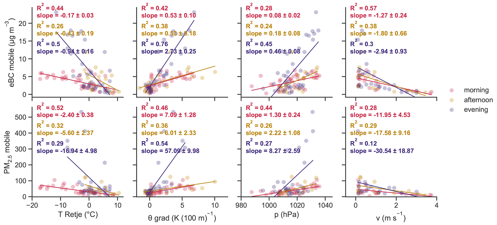
Figure 8Linear correlations between the temperature measured at the Retje station (T Retje), potential temperature gradient (θ grad), atmospheric pressure (p), and wind speed measured at Hrib (v) with mobile eBC and PM_2.5 mass concentrations inside the cold air pool (CAP).

Download

Temperature dependence of eBC is higher for evening runs (R²=0.5) compared to morning (R²=0.44) and afternoon (R²=0.26) runs. However, for PM_2.5, the correlation is stronger in the morning (R²=0.5) than in the evening and in the afternoon (R²=0.3). However, the gradient of the linear regression line is, like eBC, steepest in the evening. With a temperature decrease of −1 ^∘C, eBC and PM_2.5 are reduced by 14 %.

Despite not being the most representative location of wind measurements for the atmospheric conditions inside the CAP, wind-speed dependence of eBC and PM_2.5 obtained with mobile measurements was confirmed as well. Correlation is better for eBC than for PM_2.5, and it is strongest for the morning runs (R²=0.6 for eBC and R²=0.3 for PM_2.5). Nonetheless, the reduction in pollutant levels in the hollow per 1 m s⁻¹ of wind speed is higher in the evening (−40 %) compared to afternoon and morning runs (from −22 % to −30 %).

Unlike the other meteorological variables, the correlation between the pollutant levels and the potential temperature gradient of the hollow is strongest in the early evening, with R²=0.8 for eBC and R²=0.5 for PM_2.5. During this time, the increase in the pollutant levels is also 63 % to 72 % higher compared to the morning and afternoon runs. The change in pollutant mass concentrations in the evening is comparable to those induced by wind speed. However, the significance of the wind-speed model is low, with R² from 0.12 to 0.3.