the Creative Commons Attribution 4.0 License.
the Creative Commons Attribution 4.0 License.
 | 01 Mar 2021
Automated time–height-resolved air mass source attribution for profiling remote sensing applications
Patric Seifert
Holger Baars
Athena Augusta Floutsi
Zhenping Yin
Johannes Bühl
Height-resolved air mass source attribution is crucial for the evaluation of profiling ground-based remote sensing observations, especially when using lidar (light detection and ranging) to investigate different aerosol types throughout the atmosphere. Lidar networks, such as EARLINET (European Aerosol Research Lidar Network) in the frame of ACTRIS (Aerosol, Clouds and Trace Gases), observe profiles of optical aerosol properties almost continuously, but usually, additional information is needed to support the characterization of the observed particles. This work presents an approach explaining how backward trajectories or particle positions from a dispersion model can be combined with geographical information (a land cover classification and manually defined areas) to obtain a continuous and vertically resolved estimate of an air mass source above a certain location. Ideally, such an estimate depends on as few as possible a priori information and auxiliary data. An automated framework for the computation of such an air mass source is presented, and two applications are described. First, the air mass source information is used for the interpretation of air mass sources for three case studies with lidar observations from Limassol (Cyprus), Punta Arenas (Chile) and ship-borne off Cabo Verde. Second, air mass source statistics are calculated for two multi-week campaigns to assess potential observation biases of lidar-based aerosol statistics. Such an automated approach is a valuable tool for the analysis of short-term campaigns but also for long-term data sets, for example, acquired by EARLINET.
- Article
(17744 KB) -
Supplement
(21516 KB) - BibTeX
- EndNote


Tracing air mass transport through a turbulent atmosphere is (still) a complex problem, especially since the transport of aerosols and, consequently, the interactions with clouds, precipitation and radiation are required to capture the 4D history of an air parcel. When it comes to practical application, such as the analysis of aerosol observations or aerosol–cloud interaction studies, the ease of interpretation is often hindered by the amount of data that needs to be considered.
The European Research Infrastructure on Aerosol, Clouds and Trace Gases (ACTRIS) aims at investigating short-lived components in the atmosphere, among them aerosols and clouds. As part of ACTRIS, the European Research Lidar Network, EARLINET (Pappalardo et al., 2014), operates lidar systems at more than 25 stations to observe atmospheric states and compositions up to 30 km height. The complementary network of Cloudnet (Illingworth et al., 2007) utilizes continuous synergistic observations of ground based instruments such as ceilometers, cloud radars, microwave radiometers and Doppler wind lidars to provide comprehensive cloud observations within Europe and at key regions in the climate system. Both networks, as part of ACTRIS, need additional, continuous information about air mass sources to interpret the observations. Identifying the air mass source region supports the characterization of new particles, e.g., during volcanic eruptions (Pappalardo et al., 2013) or strong wildfires injecting aerosol into the stratosphere (Baars et al., 2019). Also, for aerosol typing (e.g., Amiridis et al., 2015; Wandinger et al., 2016; Papagiannopoulos et al., 2020; Nicolae et al., 2018; Mylonaki et al., 2020), air mass sources can provide an important constraint. Furthermore, operational height-resolved air mass source information could improve warning applications for hazardous events, as demonstrated for EARLINET in the frame of the European EUNADICS-AV exercise (European Natural Disaster Coordination and Information System for Aviation; Papagiannopoulos et al., 2020).
Models that simulate air mass transport can be broadly grouped into trajectory models and particle dispersion models (overview provided by Fleming et al., 2012). Trajectory models calculate the transport of a single air parcel imposed by the mean meteorological fields. The model simulations can be run either forward or backward in time, providing information about the source and the destination of the air mass, respectively, after a given transport time. Turbulence and vertical motion during the transport are usually parameterized on the grid scale. Commonly used models are HYSPLIT (Hybrid Single-Particle Lagrangian Integrated Trajectory model; Stein et al., 2015), FLEXTRA (flexible trajectories; Stohl et al., 1995) and LAGRANTO (Lagrangian analysis tool; Wernli and Davies, 1997; Tarasova et al., 2009). Due to the rather simple approach, the results are quite uncertain (Seibert, 1993; Polissar et al., 1999), but computational requirements are comparably low. A straightforward approach for representing some of the variability is calculating spatial or temporal ensembles of the trajectories (Merrill et al., 1985; Kahl, 1993; Draxler, 2003). Lagrangian particle dispersion models (LPDM), with a large number of particles, are set up to cover turbulent and diffusive transport even more realistically (Stohl et al., 2002). The fate of each particle is tracked individually, allowing more variability to be included into the transport simulation. A frequently used LPDM is FLEXPART (FLEXible PARTicle dispersion model; Pisso et al., 2019).
Generally, the representation of chaotic motion in the atmosphere improves with larger ensembles of trajectories or increasing numbers of particles. But, with dozens to hundreds of air parcel locations available, interpretation rapidly becomes cumbersome. A number of infinitesimally small air parcels grouped together gives an air mass, which is a larger volume of air with similar properties. Residence times are a well-established technique for attributing regional information to air mass properties, such as being laden with aerosols, moisture or trace gases (Ashbaugh, 1983; Ashbaugh et al., 1985).
Using backward simulations of air parcel positions, analysis of the residence time yields useful information about the potential source region of an observed air mass. The basic assumption is that the longer an air parcel was present in a certain region, the more likely it will be influenced by the surface characteristics. Hence, the dimensionality of an air parcel's 4D location can be reduced to the residence time. Approaches for clustering backward trajectories by direction, source regions or latitude are widely used. The majority focus on the interpretation of time series observations at single heights – mostly close to ground (e.g., Escudero et al., 2011), for aircraft intersects (e.g., Paris et al., 2010), or over a whole region (Lu et al., 2012). More sophisticated approaches blend the residence time with actual concentration measurements (Stohl, 1996; Heintzenberg et al., 2013). However, these approaches require continuous concentration time series, which are generally not available for remote sensing observations. Furthermore, any profile information above the measurement site is neglected.
When interpreting ground-based remote sensing observations, as obtained from aerosol lidars or cloud radars, the air mass sources have usually been assigned by manually selected periods (time and height above ground) that seem interesting for further investigation and calculation of backward transport for those specific cases (e.g., Müller et al., 2007; Mattis et al., 2008). If air mass source estimates are required for longer time periods or multiple heights, calculating, visualizing and interpreting the results become tedious. Hence, a continuous, computationally efficient, easy to interpret and automated air mass source estimate is required. To be broadly and easily applicable, such a source estimate should not require extensive a priori information, such as clusters of trajectories or potential source contribution functions. The required approach is intended to also be simpler than using a coupled aerosol model, such as CAMS (Copernicus Atmosphere Monitoring Service; Flemming et al., 2017), COSMO-MUSCAT (COnsortium for Small-scale MOdeling MUltiScale Chemistry Aerosol Transport Model; Dipu et al., 2017) or ICON-ART (ICOsahedral Nonhydrostatic Aerosols and Reactive Trace gases; Rieger et al., 2015). Although these models can provide profiles of atmospheric composition, they usually do not provide information on the source.
Herein, we propose a combination of automated backward trajectory calculations and geographical information for the setup of a simple, spatiotemporally resolved air mass source attribution scheme. As a proxy for geographical information, two products are used, namely a land cover classification mask and manually defined geographical areas. The methodology is described in Sect. 2. A comprehensive, easy-to-use software package is also provided. Earlier versions were already used in Haarig et al. (2017), Foth et al. (2019) and Floutsi et al. (2021). Afterwards, two applications illustrate the potential use cases. In the first example, the temporal and vertical evolution of the air mass source is analyzed for three lidar observations of different aerosol conditions from Limassol (Cyprus), Punta Arenas (Chile) and on board R/V Polarstern off Cabo Verde. In the second example, vertically resolved air mass source statistics are used to assess potential observation biases of long-term lidar-based aerosol statistics. Two multi-week campaigns of the PollyNET (Baars et al., 2016), as a part of EARLINET, are presented, namely Finokalia (Greece) and Krauthausen (Germany).
In a conceptualized view, properties of an air parcel arriving over a location of interest are characterized by a certain surface type if the air was close to the surface during its traveled path. The proximity to the surface can be parameterized as a reception height, which depends on the mixing state of the atmosphere at this location and on the type of aerosol particles that could potentially be emitted (i.e., mineral dust or sea salt). Conceivable choices for the reception height are the model-derived depth of the atmospheric boundary layer or fixed thresholds. As a first estimate for the identification of possible surface effects on an air parcel, 2 km is widely used (Val Martin et al., 2018). It is assumed that the longer an air parcel resides close to the surface, the more likely it will acquire the aerosol footprint of the surface. The residence time – the total time an air parcel spent over a certain surface and below the reception height – is a first hint of the aerosol characteristics of the air parcel.
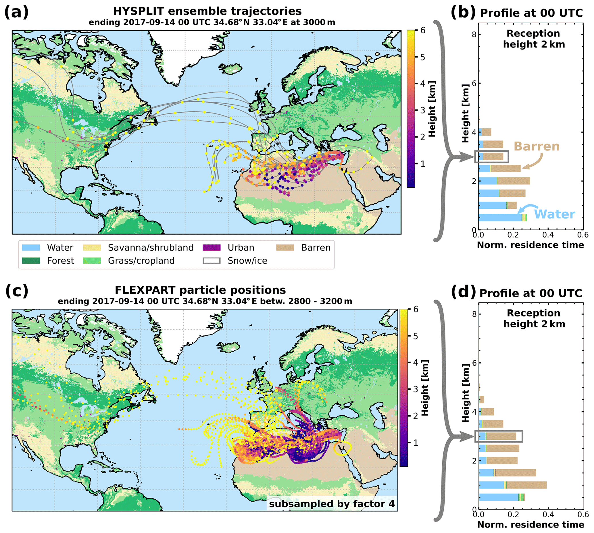
Figure 1Example of how the residence time profile is calculated. HYSPLIT ensemble backward trajectories (a) and FLEXPART particle positions (c) ending above Limassol on 14 September 2017, 00:00 UTC, at 3 km height. The number of FLEXPART particles is reduced by a factor of 4 in this visualization (i.e., 10 000 instead of 40 000). A time-resolved version with all particles is provided in the Supplement. Air parcel height is color coded. The simplified MODIS land surface classification (Fig. 2) is shown in the background. The profiles of normalized residence time with a reception height threshold of 2 km for HYSPLIT ensemble trajectories (b) and FLEXPART particle positions (d) are shown.
The transport pathway of an air mass arriving over the site can be computed using either mean-wind trajectories or a particle dispersion model. Both approaches can be used with the method proposed in this study. Mean wind trajectories for the past 10 d are calculated using HYSPLIT (Stein et al., 2015). To account for variability, ensemble trajectories consisting of 27 members, spaced 0.3∘ horizontally and 220 m vertically around the end point, are used (Fig. 1a). Meteorological input data for HYSPLIT are obtained from the Global Data Assimilation System data set at 1∘ horizontal resolution (GDAS1) and are provided by the Air Resources Laboratory (ARL) of the U.S. National Weather Service's National Centers for Environmental Prediction (NCEP; ARL Archive, 2019). The location of the air parcel is stored in 1 h steps. A more realistic representation of turbulence and mixing can be achieved using a LPDM, which simulates the pathway of hundreds to thousands of particles. Here, the most recent version of FLEXPART (Stohl et al., 2005; Pisso et al., 2019) is used. Meteorological data are obtained from the GFS (Global Forecast System) analysis at a horizontal resolution of 1∘ (NCEP et al., 2000). For each height, 500 particles are used, with the particle positions being stored every 3 h. These simulations are run every 3 h, with height steps of 500 m for the whole period of interest.
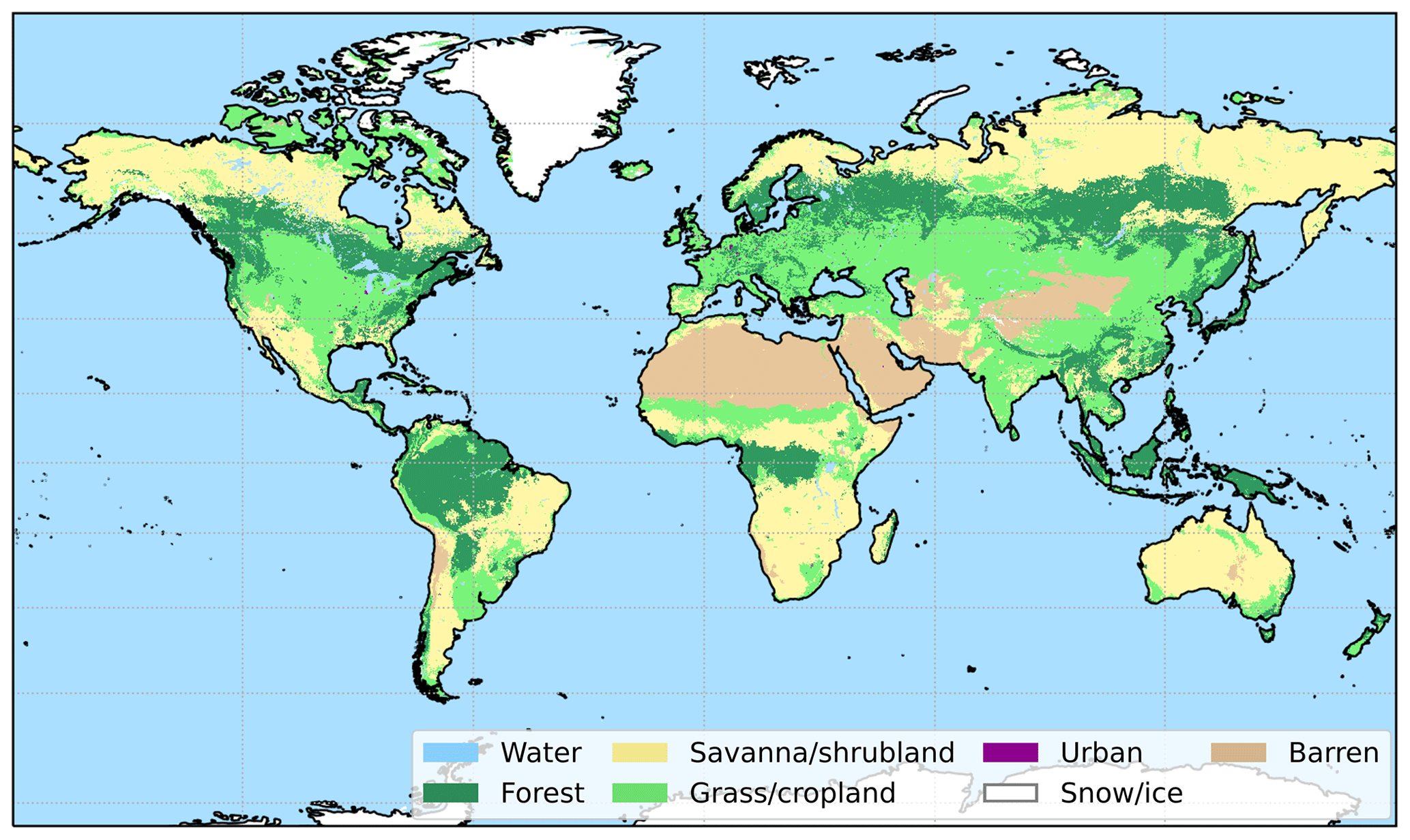
Figure 2The simplified MODIS land cover classification. Details are given in the text.
In this work, the surface is classified by two methods. The first method is based on a simplified version of the MODIS land cover classification (Friedl et al., 2002; Broxton et al., 2014). The 17 categories of the original data set are grouped into seven categories according to Table 1 in order to allow for robust statistics in the output (Fig. 2). Additionally, the horizontal resolution is reduced to 0.1∘. The categories do not resolve the annual cycles, for example, due to growing seasons. The second method involves custom defined areas as polygons, named according to their geographical context (Fig. 3). These areas can be tailored to the measurement location and/or scientific interest.
Table 1Overview of how the MODIS land surface categories translate into the simplified categories used in this study. MODIS category numbers as in Broxton et al. (2014).
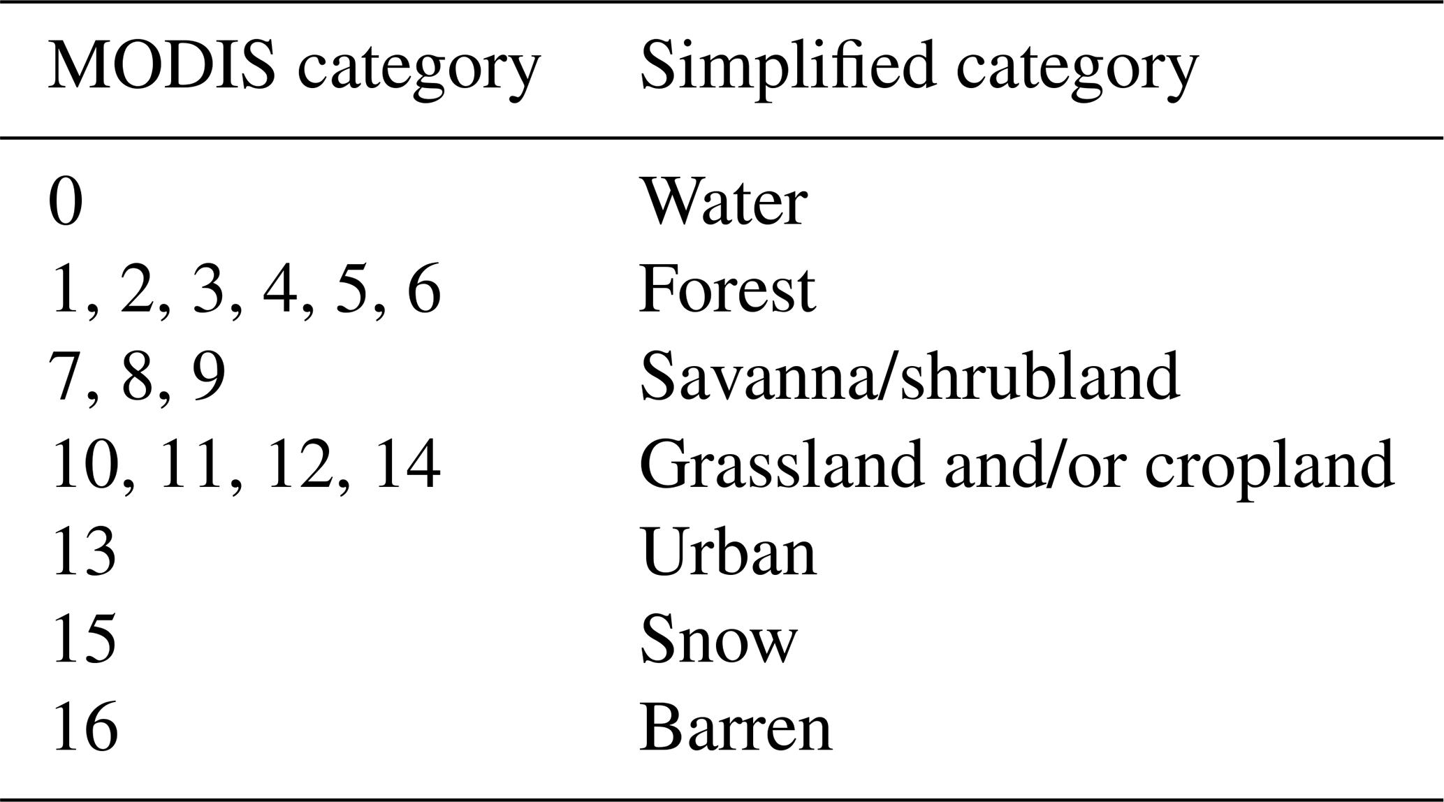
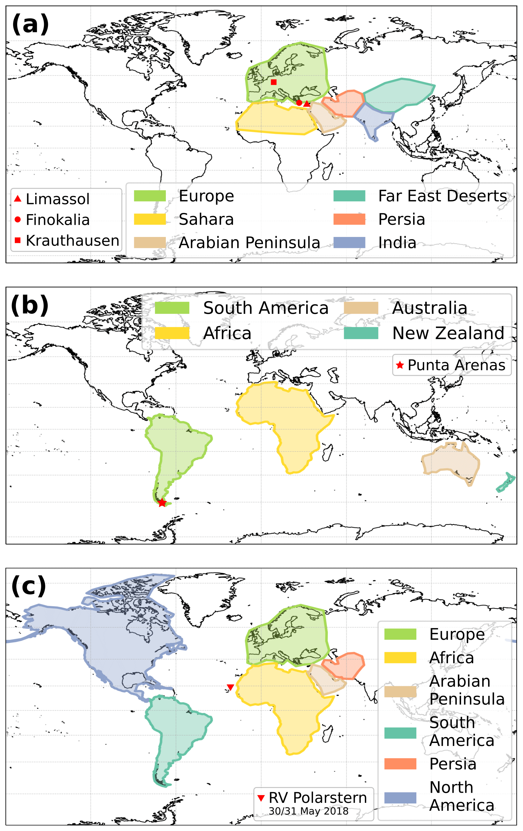
Figure 3The custom defined geographical areas for Limassol, Finokalia, Krauthausen (all shown in a), Punta Arenas (b) and the Atlantic transit (c). Locations of the sites are also marked on the respective maps.
The residence times at each time and height step are summed for each land cover class or polygon, where the air parcel was below the reception height. Within this study, the widely applicable reception height threshold of 2 km is used (Val Martin et al., 2018). Different settings can be easily applied to study events which are entrained at greater heights, such as wildfire smoke emission or volcanic eruptions. The vertical air mass transport during such events is usually not accurately covered by atmospheric models. Setting the reception height to the maximum emission height of such events (as can be estimated, e.g., from satellite observations) can bypass the uncertainties in the modeled vertical motion. The residence times for each category and each height can then be visualized as a profile (Fig. 1b). Where the residence time is 0, no air parcels were observed below the reception height during the duration of the backward simulation. In the example shown in Fig. 1b, above 5 km height, no air masses resided at heights below 2 km above the ground in the previous 10 d. The theoretical maximum residence time (in hours) depends on the number of trajectories or particles n, the duration of backward calculation d in days and the interval of output Δo in hours as follows:
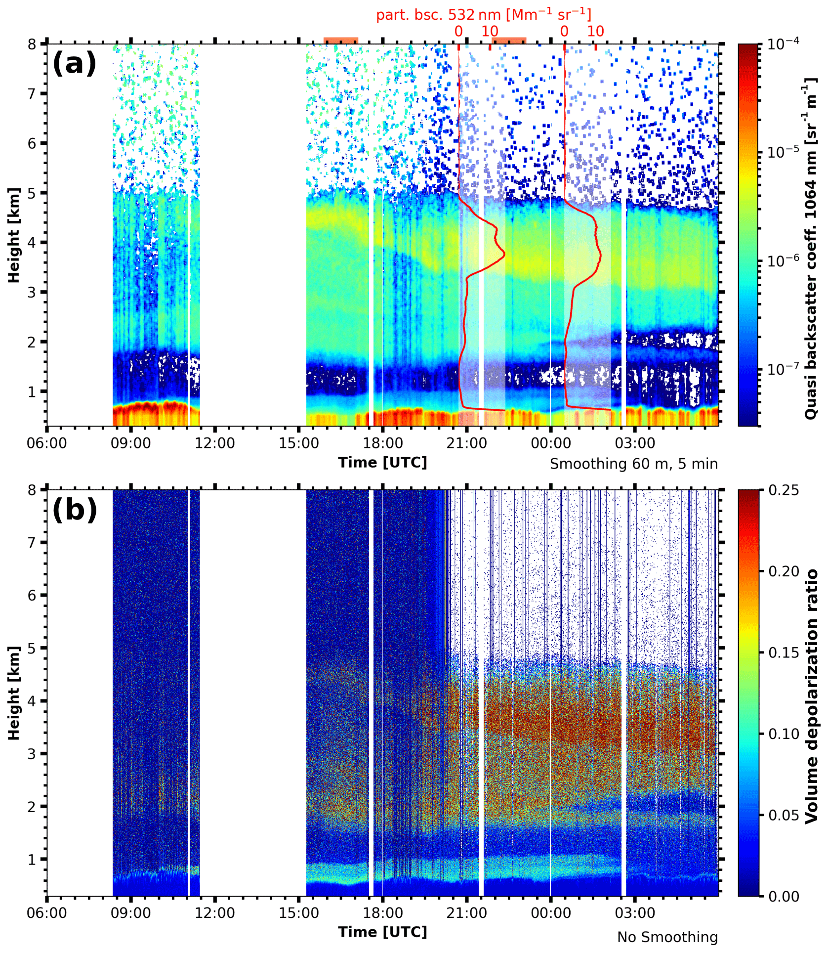
Figure 4(a) Quasi particle backscatter coefficient at 1064 nm observed by PollyXT on board R/V Polarstern close to Cabo Verde on 30 and 31 May 2018. Moving average smoothing of eight range bins (60 m) and 10 temporal bins (5 min) was applied. The red overlays show the Klett-derived particle backscatter coefficient from the automated algorithm at 532 nm. The time period of manual analysis (see text) is marked by a horizontal orange bar. (b) Volume depolarization ratio at 532 nm for the same period. No smoothing was applied.
To illustrate the temporal evolution, successive air mass source profiles can be shown one after another. This visualization condenses the 4D history of a multitude of trajectories (or thousands of particle positions) to a quickly understandable summary, which structures information on air mass source into a time–height cross section. Such a format is usually obtained from vertically or nadir-pointed active ground-based remote sensing observations (e.g., Fig. 4).
The air mass source estimate is used to interpret observations conducted with the PollyXT lidar (Engelmann et al., 2016). PollyXT is equipped with backscatter channels at 1064, 532 and 355 nm and Raman and depolarization channels at the shorter two wavelengths. The optical properties are derived using the automated PollyNET retrieval (Baars et al., 2016, 2017; Yin and Baars, 2020) and manual analysis of single profiles. One product of the PollyNET retrieval is the quasi backscatter coefficient, where the attenuated backscatter is corrected for molecular extinction. For this approach, the background, range and dead-time-corrected lidar profiles are normalized by the so-called lidar calibration parameter (also sometimes called the lidar constant even though it is not constant) which is derived from Raman or Klett retrievals (see Baars et al., 2016). This normalization gives the attenuated backscatter coefficient from ground (note that, for the same atmospheric scene, the attenuated backscatter measured from ground is different to the one measured from space as it is not corrected for attenuation by molecules and particles). The molecular contribution to the atmospheric backscattering and extinction can be calculated from pressure and temperature profiles; the attenuated backscatter coefficient is corrected for the molecular scattering. Furthermore, an assumption of a fixed lidar ratio is applied on the attenuated backscatter corrected for molecular contribution to account for a first guess of the particulate attenuation. This procedure gives the quasi particle backscatter coefficient, which is a good proxy for the real particle backscatter coefficient that cannot yet be obtained at a high temporal resolution for all atmospheric scenes. More details are covered in Baars et al. (2017).
PollyXT was deployed to various field campaigns and longer-term measurements during the last 15 years (Baars et al., 2016). A broad variety of meteorological conditions and aerosol regimes was covered. The multi-wavelength observations of PollyXT contain unique fingerprints of the observed aerosol types from different source regions (Illingworth et al., 2015).
In Sects. 4 and 5, the air mass source attribution will be applied to selected case studies and measurement campaigns in order to demonstrate its applicability for determinating the air mass source regions and for the estimate of potential observation biases. The case studies are chosen from deployments of PollyXT to Limassol (Cyprus; 34.7∘ N, 33.0∘ E; 12 m above sea level (a.s.l.); October 2016 to March 2018), Punta Arenas (Chile; 53.1∘ S, 70.9∘ W; 10 m a.s.l.; November 2018 and ongoing) and the Atlantic transit of R/V Polarstern in 2018 when passing Cabo Verde (18.1∘ N, 21.3∘ W to 21.3∘ N, 20.8∘ W). The estimate of potential observation biases is done for two multi-week campaigns. One at Krauthausen (Germany; 50.9∘ N, 6.4∘ E; 99 m a.s.l.) took place for 8 weeks in April–May 2013 and the second one was at Finokalia (Greece; 35.3∘ N 25.7∘ E; 250 m a.s.l.) for 6.5 weeks in June–July 2014.
4.1 Saharan dust off the coast of West Africa
A lofted layer of dust was observed on 30 and 31 May 2018 by a PollyXT system on board R/V Polarstern (Strass, 2018) as the ship steamed between Cabo Verde and the African mainland (18.1∘ N, 21.3∘ W to 21.3∘ N, 20.8∘ W) on her transit north from Punta Arenas (Chile) to Bremerhaven (Germany). A detailed description of the event and optical properties of the observed aerosol were already reported by Yin et al. (2019).
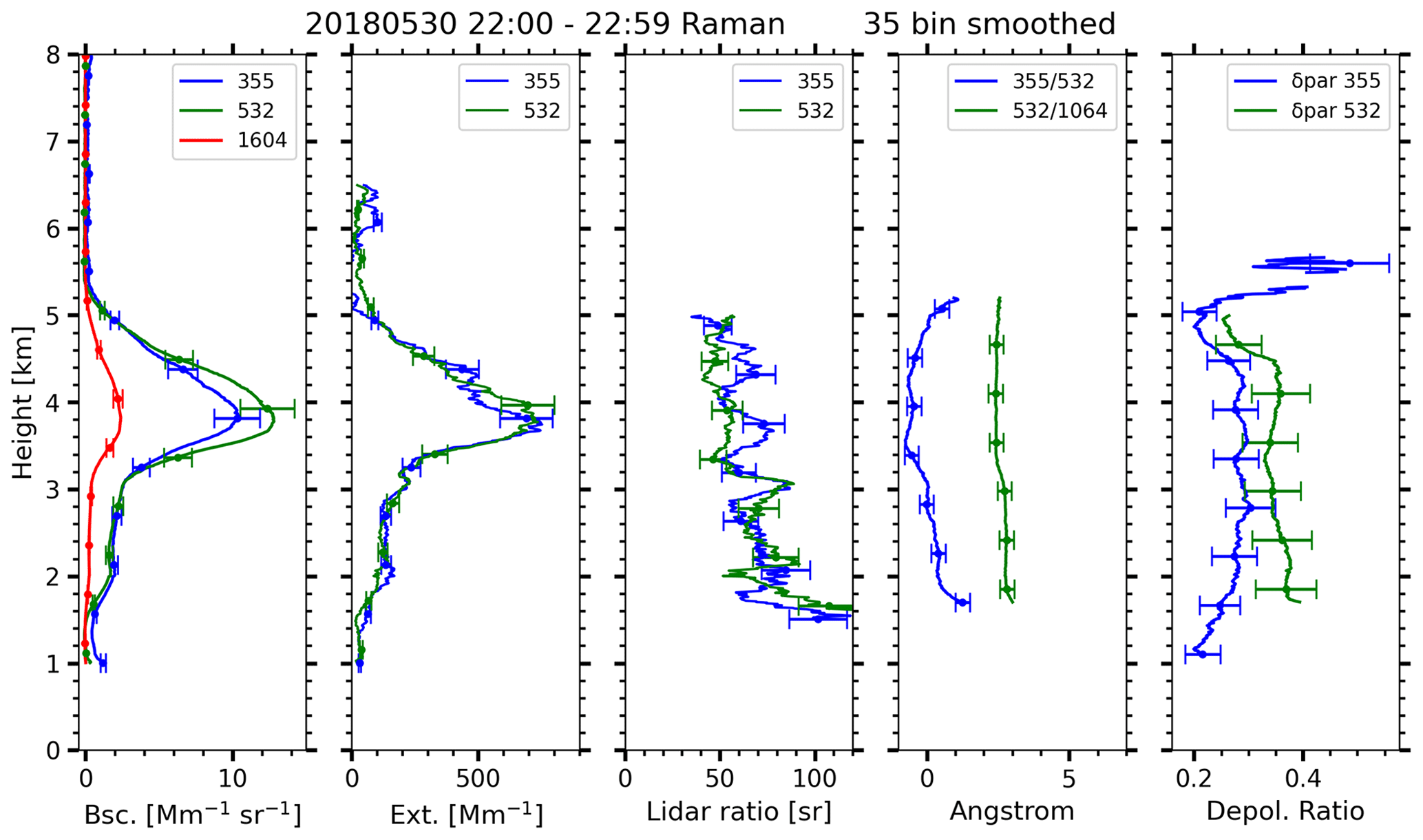
Figure 5Profiles of optical properties on 30 May 2018, between 22:00 and 22:59 UTC, manually derived with the Raman method. A vertical smoothing of 35 bins (262.5 m) was applied.
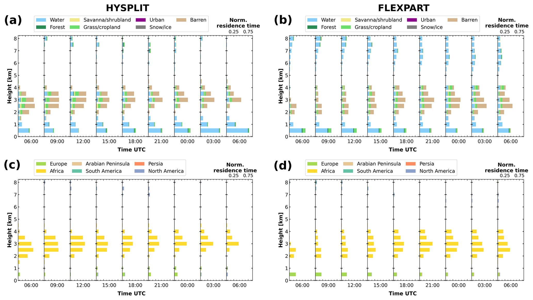
Figure 6Air mass source estimate from 06:00 UTC on 30 May 2018 to 06:00 UTC on 31 May 2018 for the land surface classification (a, b) and the named geographical areas (b, d), based on HYSPLIT ensemble trajectories (a, c) and FLEXPART particle positions (b, d).
Figure 4 illustrates the temporal evolution of the observed aerosol plume by means of a time–height cross section of the 1064 nm quasi particle backscatter coefficient for the time period from 30 May 06:00 UTC to 31 May 06:00 UTC. Yin et al. (2019) already discussed this case, especially the period from 16:00 to 17:00 UTC (their Fig. 14). Optical parameters from the Raman analysis during the following night from 22:00 to 23:00 UTC are shown in Fig. 5 (period marked in Fig. 4a with a horizontal orange bar). According to the optical properties, Yin et al. (2019) argued that the lowest 1 km was dominated by marine particles and a certain contribution from European continental aerosol. Patchy, liquid clouds were observed at the boundary layer top, especially around 09:00 and 19:00 UTC. At larger heights, between 1.8 and 5.2 km height, a Saharan dust plume with extinction values as large as 700 Mm−1 was present. Lidar ratios were 60 sr and particle linear depolarization ratios at 532 nm of 0.35. The low Ångström exponent between the 532 and 355 nm backscatter coefficients is consistent with values reported by Veselovskii et al. (2016) and Rittmeister et al. (2017). Yin et al. (2019) corroborate their findings by ensemble calculations of HYSPLIT backward trajectories for selected arrival heights and times. However, this way of presentation is rather selective, as information for different heights and times can hardly be shown. This is where the benefit of the continuous air mass source estimate becomes evident. Figure 6 presents the results of the air mass source estimate for the land surface classification and geographical areas for both the HYSPLIT (Fig. 6a, c) and the FLEXPART simulations (Fig. 6b, d). The estimates based on HYSPLIT and FLEXPART show a good general agreement. The heights and times of certain surface types and geographical regions agree qualitatively. Before 12:00 UTC on 30 May 2018, FLEXPART derived a lower residence time from barren and grassland regions or Africa, respectively. With respect to Fig. 4, this seems to be reasonable as the layer was rather faint at the beginning of the shown measurement period. Besides this difference, both the HYSPLIT and FLEXPART approaches provide a concise picture of the likely source regions of the observed aerosol. Below 1.5 km height, the air mass was marine dominated, with a small contribution of European grass and/or cropland. At heights between 2 and 4 km, barren areas from Africa are the main source, but a considerable fraction is also attributed to African grass/cropland and savanna. This finding supports the observations presented by Yin et al. (2019), who already discussed that there was likely a small non-dust fraction in the upper layer as the particle depolarization ratio profile was not constant at all heights. A potential reason for the observed discrepancy in the observations from pure dust conditions could be the presence of wildfire smoke stemming from the crop/grassland and savanna. In comparison to the lidar observations, the top of the layer was slightly underestimated by the air mass source estimate. The temporal extent is also fully captured. Variability in backscatter within the layer is not represented by the air mass source estimate because the strength of dust mobilization is insufficiently parameterized by the reception height. However, the air mass transport is correctly covered by both estimates. Interestingly, the air mass source estimation for this case provides some information with an added value with respect to the lidar observations. As both HYSPLIT and FLEXPART approaches indicate, North American air masses were present in the upper troposphere during the time of the observation, which, however, had too low an aerosol load to be detectable by the PollyXT lidar.
4.2 Saharan and Arabian dust at Limassol, Cyprus
On 14 September 2017 an upper level shortwave trough moved eastward from the Aegean Sea towards Cyprus. Above 1 km height, the wind turned from southwest to south during the course of the day, with velocities ranging between 5–15 m s−1, whereas, below the 1 km height, wind velocity was lower and the direction was more variable.
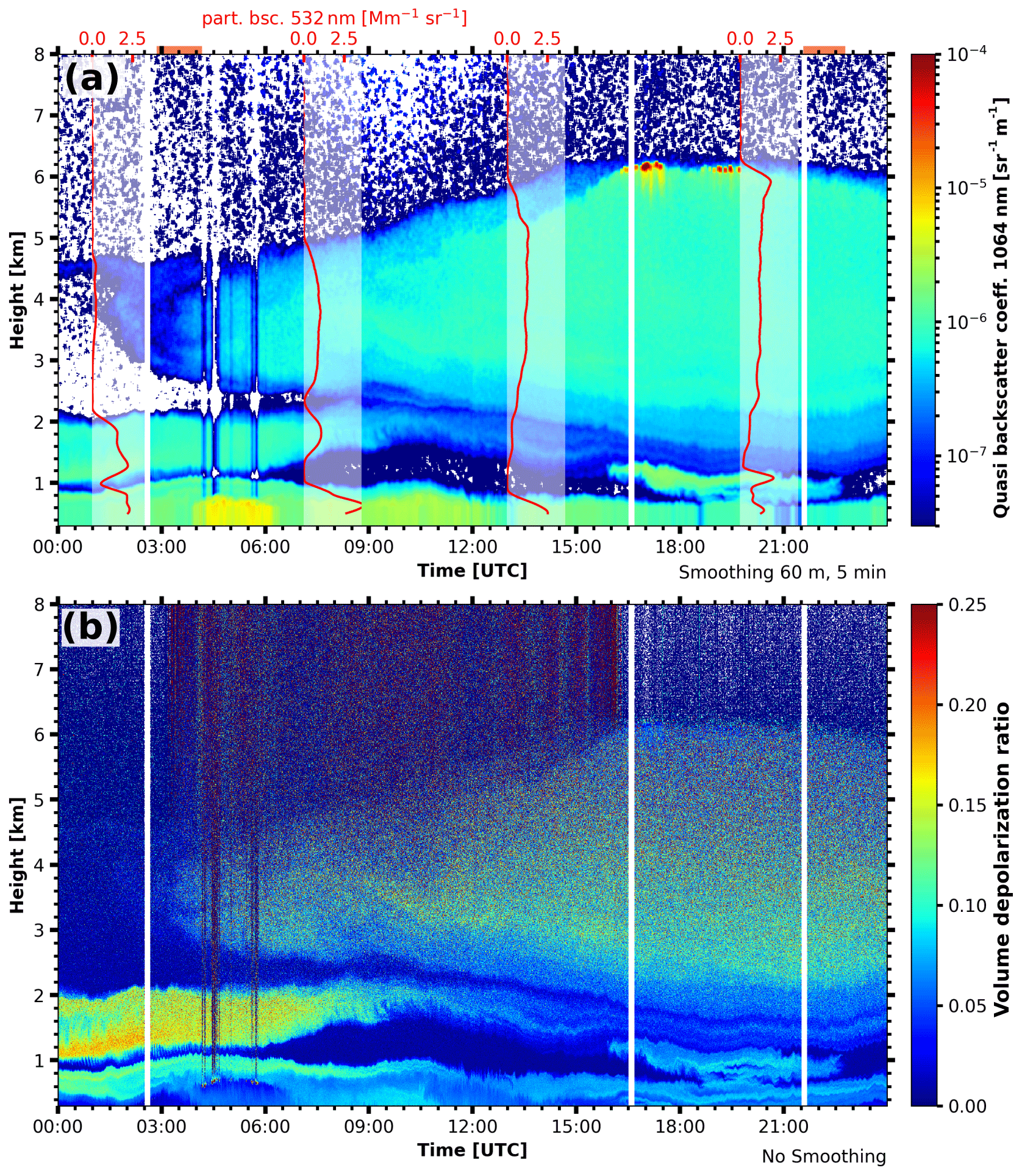
Figure 7(a) Quasi particle backscatter coefficient at 1064 nm observed by PollyXT at Limassol on 14 September 2017. Moving average smoothing of eight range bins (60 m) and 10 temporal bins (5 min) was applied. The red overlays show the Klett-derived particle backscatter coefficient at 532 nm. The time periods of manual analysis (Figs. 8 and 9) are marked by horizontal orange bars. (b) Volume depolarization ratio at 532 nm for the same period. No smoothing was applied.
The time–height cross section of quasi particle backscatter observed by PollyXT at Limassol shows two pronounced aerosol layers above the boundary layer (Fig. 7). The first layer was observed between 1 and 2 km height from 00:00 to 09:00 UTC and a second, thicker layer after 03:00 UTC. Until nighttime, this layer increases in thickness from bases at 3 km and tops at 4.5 km height to bases at 1.2 km and tops at 6.5 km height. The boundary layer itself is also laden with aerosols and shows significant backscatter below 1 km height.
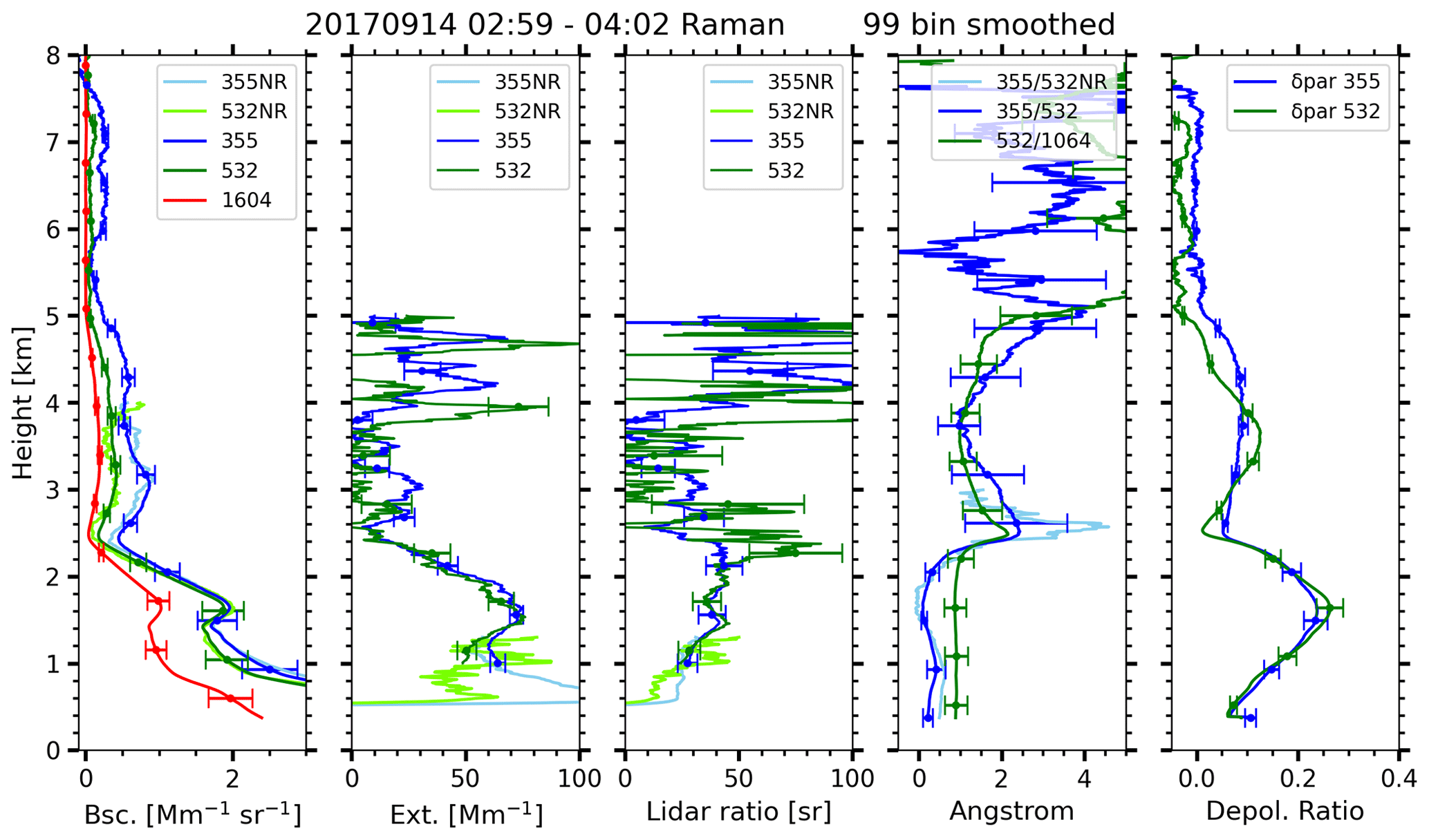
Figure 8Profiles of optical properties on 14 September 2017, between 02:59 and 04:02 UTC, manually derived with the Raman method. A smoothing of 99 range bins (742.5 m) was applied. The abbreviation NR indicates the profiles observed with the larger field of view near-range telescope.
The optical parameters of the aerosol plume were analyzed for two periods, namely 02:59–04:02 UTC in the morning and 21:41–22:39 UTC in the evening (periods marked in Fig. 7a with horizontal orange bars). The profiles from the morning period (Fig. 8) show, for the lower layer at 1.8 km height, particle depolarization ratios of 0.25 (355 and 532 nm) and low Ångström values and lidar ratios around 40 sr (355 and 532 nm). These optical parameters and their independence of wavelength are typical for aerosol mixtures with a high dust fraction. Extinction in this layer peaks at 72 Mm−1 (355 and 532 nm). The second layer, above 2.5 km height, has particle backscatter values of less than 2 Mm−1 sr−1 (at 355 nm) and 0.5 Mm−1 sr−1 (at 532 nm). Ångström values are slightly higher than in the lower layer, varying between one and two. The particle depolarization ratios, at both the 355 and 532 nm wavelength, are between 0.05 and 0.10. This upper layer during the morning is already the leading edge of the second plume that increased in thickness during the day (both geometrically and optical). As shown in Fig. 7b, the volume depolarization ratio increased only slowly during the averaging period.

Figure 9Profiles of optical properties on 14 September 2017, between 21:41 and 22:39 UTC, manually derived with the Raman method. A smoothing of 99 range bins (742.5 m) was applied. The abbreviation of NR indicates profiles observed with the larger field of view near-range telescope.
During the evening (Fig. 9), the upper layer extended from 1.3 to 6 km height and shows homogeneous and mostly wavelength-independent optical properties throughout. Particle depolarization ratios were between 0.10 and 0.15, with 532 nm values slightly higher than those at 355 nm. Lidar ratios in that layer were 35 sr, typical for Middle Eastern dust (Mamouri et al., 2013; Nisantzi et al., 2015), while the particle depolarization ratio hints towards a mixture of mineral dust and anthropogenic pollution (e.g., Tesche et al., 2009).
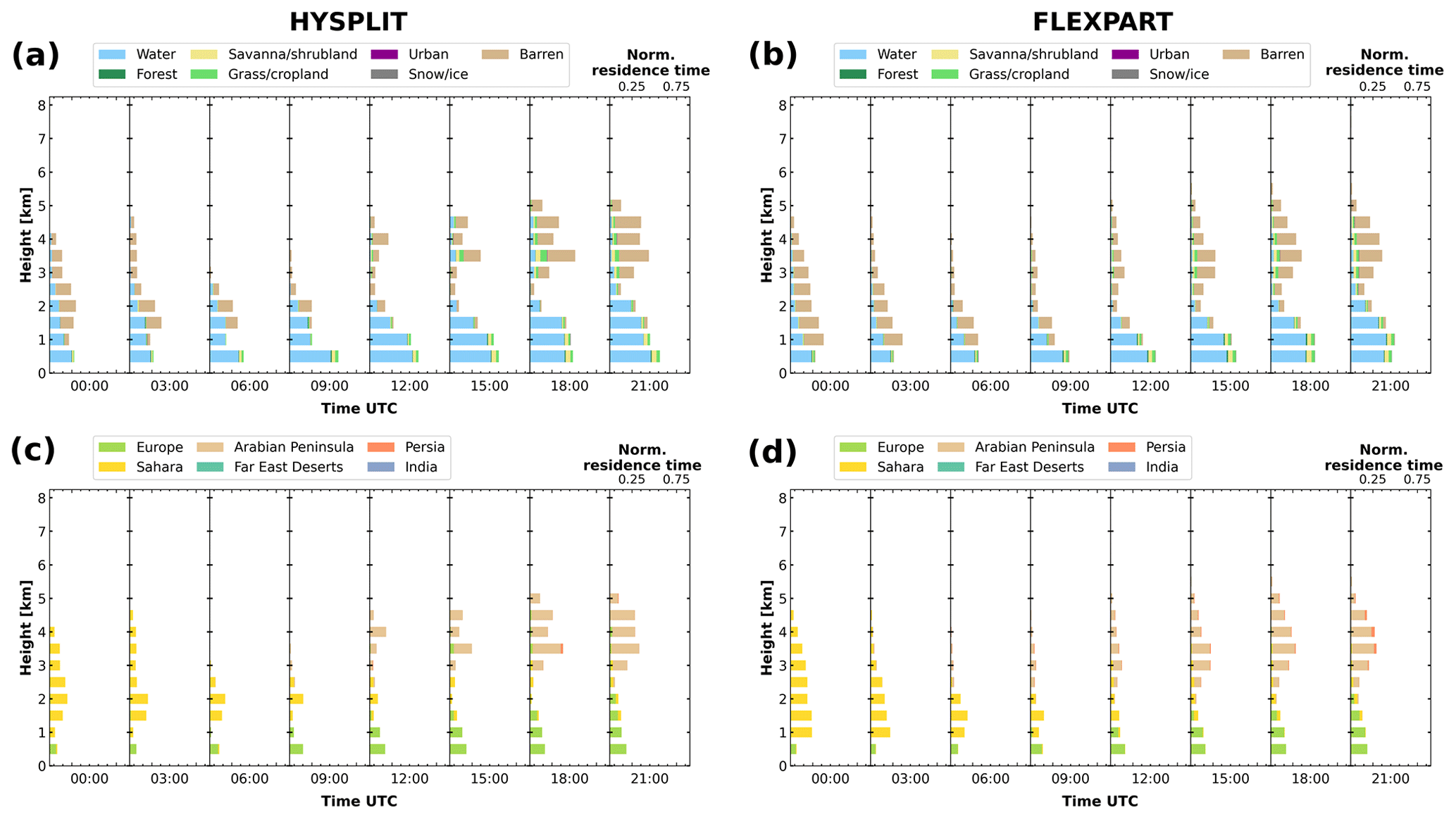
Figure 10Air mass source estimate on 14 September 2017 for the land surface classification (a, b) and the named geographical areas (b, d), based on HYSPLIT ensemble trajectories (a, c) and FLEXPART particle positions (b, d).
The air mass source estimate (Fig. 10) identifies transport from barren-ground-influenced air from the Sahara until 09:00 UTC. Later, corresponding to the change in wind direction, the source for the air aloft is identified as Arabian Peninsula but is still in the barren class. Below 1 km height, a mixture of surfaces was observed, originating mostly form Europe. Comparing the source estimate based on HYSPLIT (Fig. 10a, c) with the one from FLEXPART (Fig. 10b, d), both models agree qualitatively well again. While the general transition was captured by the source estimate, the leading edge of the Arabian Peninsula plume was observed over Limassol earlier than indicated. The increase in the thickness of this plume is represented in the source estimate as well.
4.3 Biomass burning aerosol at Punta Arenas, Chile
Punta Arenas is located in a region where the atmosphere is known to be clean and one of the least affected by anthropogenic influences (Hamilton et al., 2014). Nevertheless, events of aerosol long-range transport occur occasionally (Foth et al., 2019; Floutsi et al., 2021). Due to the large distance between Punta Arenas and the aerosol source regions, an attribution of observed aerosol events is, in general, rather complicated. The application of air mass source estimates for the characterization of an aerosol long-range transport event is presented here. An upper-level ridge was located off the Chilean coast on 20 May 2019, which also supported a surface high-pressure system. At Punta Arenas, the flow was zonal throughout the troposphere. Within that flow, long-range transport from across the Pacific Ocean occurred.
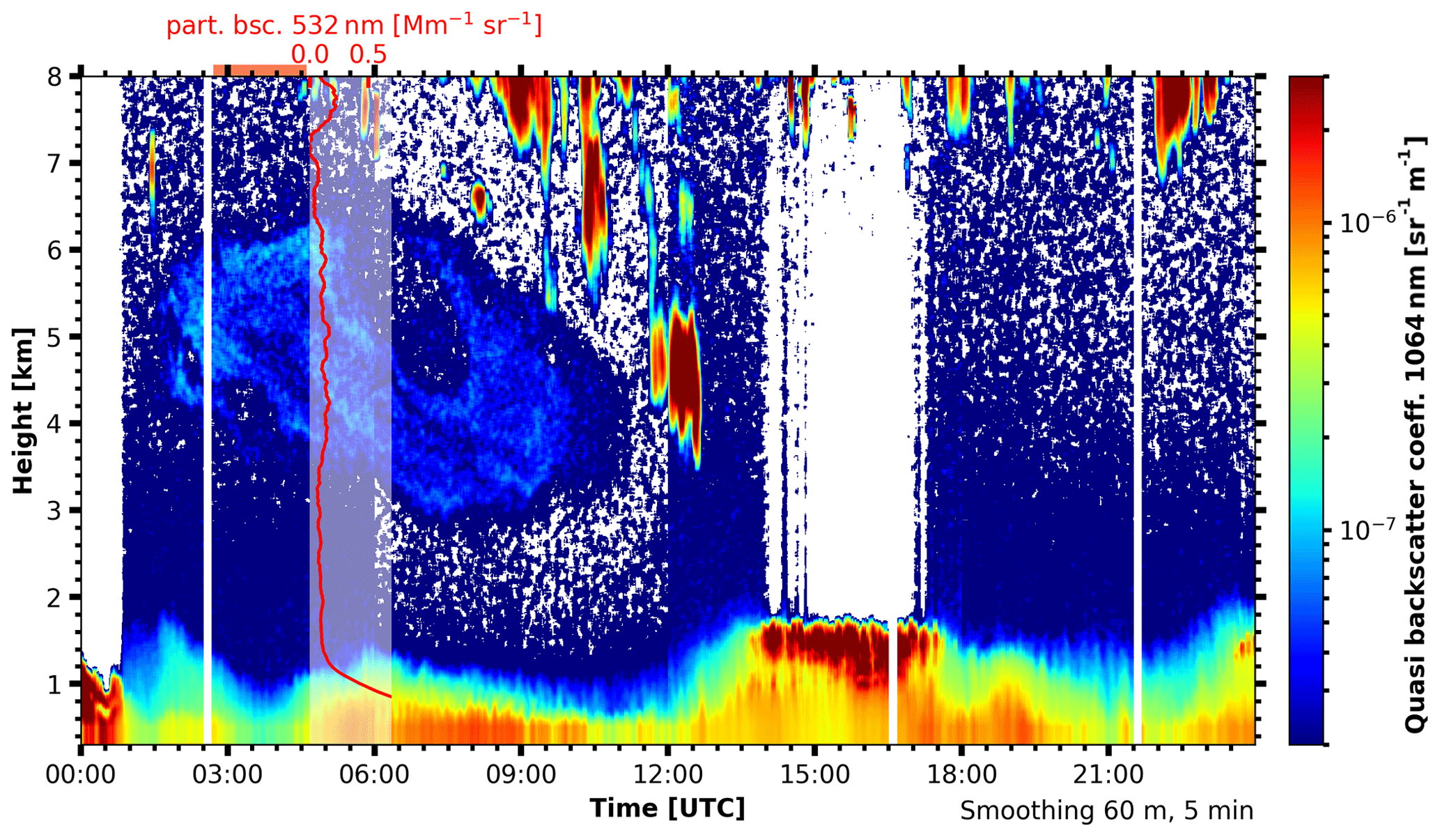
Figure 11Quasi particle backscatter coefficient at 1064 nm observed by PollyXT at Punta Arenas on 20 May 2019. Moving average smoothing of eight range bins (60 m) and 10 temporal bins (5 min) was applied. The red overlay shows the Klett-derived particle backscatter coefficient at 532 nm. The time period of the manual analysis (Fig. 12) is marked by a horizontal orange bar.

Figure 12Profiles of optical properties on 20 May 2019, between 02:50 and 04:30 UTC, manually derived with the Raman method. A smoothing of range 153 bins (1147.5 m) was applied. The abbreviation NR indicates profiles observed with the larger field of view near-range telescope.
In the PollyXT observations from 20 May 2019 a layer of increased backscatter is present from 02:00 UTC to roughly 10:00 UTC. This layer extends from 3 km to above 6 km height (Fig. 11). From 14:00 to 18:00 UTC a low-level liquid cloud was observed at 1.5 km height. The cloud was optically thick enough to significantly attenuate the laser beam, causing a lack of signal above the cloud's top. Occasional cirrus clouds also enhanced the backscatter in the free troposphere, e.g., at 12:00 UTC, between 4 and 5 km. The values of particle backscatter peaked at 0.3 Mm−1 sr−1 (Fig. 12), which are significantly lower values than reported for the prior cases. In the period analyzed, extinction values were approximately 15 Mm−1, giving lidar ratios well above 50 sr and rather low linear particle depolarization ratios. Altogether, these optical parameters agree with prior findings of wildfire smoke in the troposphere (Tesche et al., 2011; Burton et al., 2012; Groß et al., 2013; Veselovskii et al., 2015).
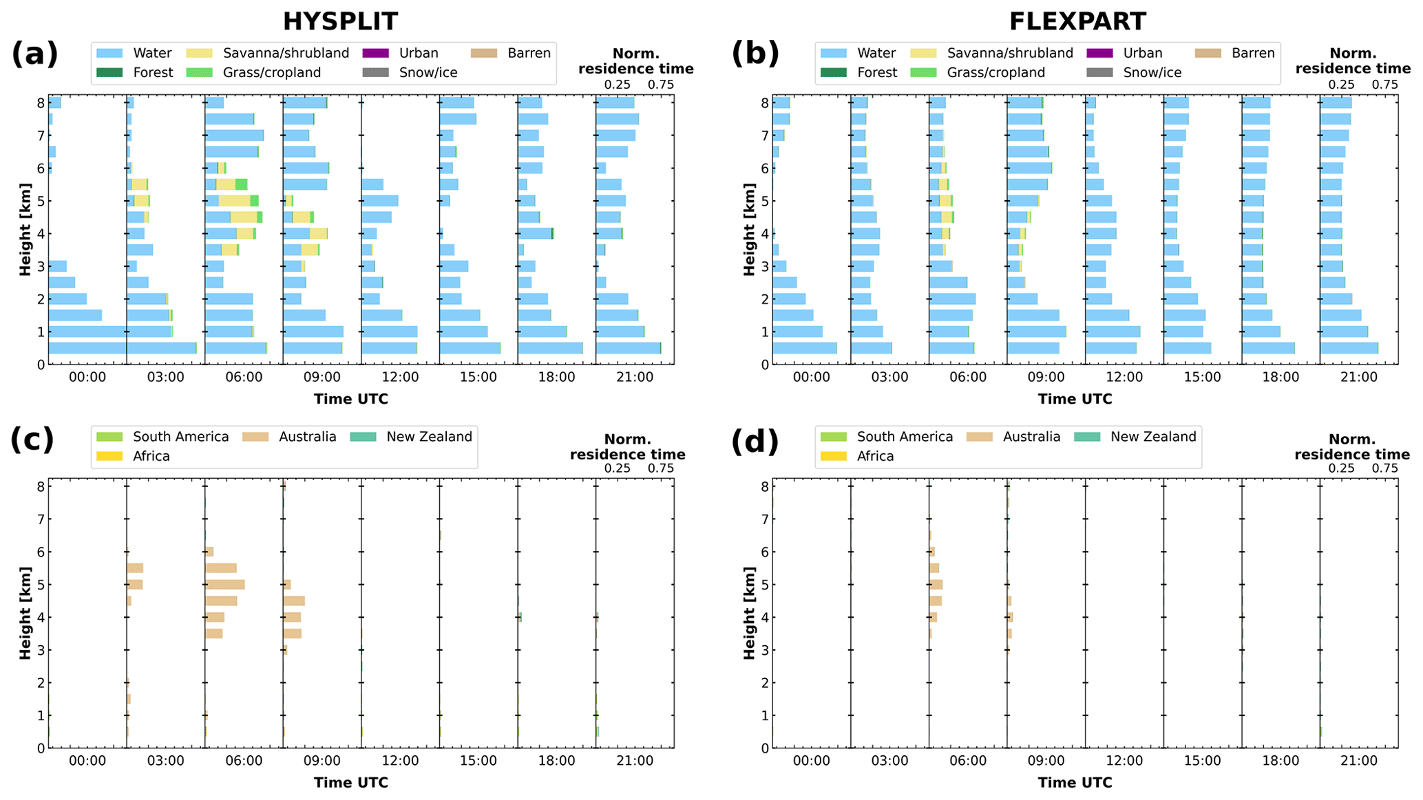
Figure 13Air mass source estimate on 20 May 2019 for the land surface classification (a, b) and the named geographical areas (b, d), based on HYSPLIT ensemble trajectories (a, c) and FLEXPART particle positions (b, d).
The air mass source estimate is also able to capture this faint aerosol layer. Fig. 13 shows that air masses from Australia were present between 03:00 and 09:00 UTC from 3 to 6 km height. In terms of land cover class, these air masses were characterized by savanna/shrubland and grass. Wildfires were active in southwestern Australia between 10 and 16 May 2019, which is also the region where the backward simulations end (Fig. A1). Apart from the described period, the air masses were solely influenced by the Southern Ocean (i.e., the water class). FLEXPART simulations (Fig. 13b, d) agree with the HYSPLIT results; however, the computed temporal extent and the residence times are slightly longer for the latter. Hence, the air mass source scheme is also capable of capturing aerosol transport at hemispheric (i.e., more than 10 000 km) scales.
Vertically resolved aerosol statistics are prone to observation biases, as they usually depend on cloud-free conditions. When clouds or precipitation are present, no aerosol properties can be obtained from optical techniques. However, respective statistics, for example, obtained from lidar observations, provide key quantities for the determination of the environmental conditions at a certain site (Matthias et al., 2004; Winker et al., 2013; Baars et al., 2016). It is therefore an open question whether the data from suitable (cloud-free) measurement periods are representative for the full observational period. Chances are that cloudy conditions are related to certain air masses which would stay unidentified in the lidar-based statistics of aerosol optical properties. One way to assess this bias is to compare the air mass residence time statistics of the full observational period with the one subsampled to the times when aerosol information is available.
When applied to lidar data, the automatically analyzed profiles of particle backscatter at 532 nm from Baars et al. (2016) are used. In their work, the raw profiles are grouped into 30 min chunks, cloud screened, averaged and analyzed by either the Klett or the Raman method to see if signal-to-noise ratio is high enough for a reference height to be set. All profiles that pass a basic quality control are then included in the backscatter statistics. Obviously, this statistic will only be intermittent, due to overcast cloud conditions or interruptions in the measurement. Subsampling the air mass source statistics is done by selecting only the air mass source profiles that are temporally close to a valid lidar profile. A time threshold of 1.5 h is used for the following statistics. However, covering representative air mass conditions is only a necessary condition and not a sufficient for obtaining representative aerosol statistics.

Figure 14Statistics of particle backscatter coefficient (a, as in Baars et al., 2016) and air mass source estimate, based on FLEXPART particle positions for the Finokalia campaign of PollyXT in June and July 2014. The land surface classification (b) and the named geographical areas (c) are shown for the full duration (solid lines) and subsampled only for the periods with available lidar data (dotted lines). The subsampled residence times are divided by the fraction of the time covered. The reception height threshold is 2 km.

Figure 15Statistics of particle backscatter coefficient (a, as in Baars et al., 2016) and air mass source estimate, based on FLEXPART particle positions for the Krauthausen campaign of PollyXT in April and May 2013. The land surface classification (b) and the named geographical areas (c) are shown for the full duration (solid lines) and subsampled only for the periods with available lidar data (dotted lines). The subsampled residence times are divided by the fraction of time covered. The reception height threshold is 2 km.
PollyXT observations at Krauthausen (Germany; April–May 2013) and Finokalia (Greece; June–July 2014) are used here. At Finokalia, 940 profiles could be analyzed with the Klett method. Hence, the particle backscatter statistic covers 457.7 h, which is 42 % of the campaign duration. The statistics of particle backscatter are shown in Fig. 14a. For the Krauthausen deployment, 315 profiles could be analyzed with the Klett method, covering 154.2 h or 11 % of the campaign. Figure 15a shows the particle backscatter statistics.
Profiles of air mass source for the Finokalia deployment are shown in Fig. 14b and c, again with a reception height threshold of 2 km. The summed residence time of the subsampled profiles is divided by the fraction of time covered to make them comparable to the full residence time. Most dominant land surface categories are water, barren ground and grass-/cropland. The residence time of air masses from barren ground shows a pronounced maximum between 2 and 6 km height. The residence time of all other categories decreases monotonically. Air masses from urban and snow- or ice-covered areas are 10–100 times less frequent than the other categories.
In terms of geographical areas (Fig. 14c), Europe is the most dominant source up to 3 km and again above 9 km height. Between 3 and 6 km height, the Sahara is the most dominant air mass source. During the campaign period, no air masses from the Arabian Peninsula, that fulfilled the <2 km criterion were transported to Finokalia.
The dominant sources are well covered by the lidar profiles in terms of land surface; only the barren class is subsampled by a factor of 10 above 6.5 km height (Fig. 14b). This agrees with the Sahara also being subsampled above that height. Air masses originating over Europe were also subsampled at heights above 5 km. An undersampling of potentially aerosol-laden air masses by the lidar statistics will cause the backscatter statistics to be biased as low values.
During the Krauthausen campaign, air masses originating over water were the most frequent ones, followed by grass-/cropland, forest, shrubland and barren ground (Fig. 15b). Again, the residence times of the barren class show a distinct peak between 6 and 8 km height. Air masses from the Sahara area agree with the barren class (Fig. 15c). As expected, Europe is the dominant air mass source in the lowest 6 km height, but due to increasing residence times with height for the Sahara source, both appear with equal frequency in the upper troposphere. In the lidar observations, Europe is potentially undersampled by 70 % between 1 and 10 km height, which is consistent with the grass/cropland and forest class also being undersampled. Barren land surfaces and the Sahara are oversampled by approximately 20 % up to 7 km height. In the lowermost 2 km height, the land surface classes urban and snow/ice also contribute to the air mass mixture and are slightly oversampled.
In this study, we propose an easy-to-use method for a continuous, height-resolved automated air mass source estimate. With the combination of air mass transport modeling and geographical information, the dimensionality can be reduced, and straightforward visualizations accelerate the interpretation of air mass origin. The air mass source estimate can be used to assist (profiling) aerosol observations, as aerosol load and characteristics are strongly controlled by surface properties and atmospheric transport. Three case studies illustrated the applicability at different sites and under different large-scale flow conditions. In a second application, we showed how the source estimate supports the interpretation of lidar case studies and how potential observation biases can be investigated for longer-term campaigns.
The major constraints of the proposed method are discussed in the following. While the air mass transport itself is generally covered well by trajectory models or LPDMs, linking it to aerosol properties has to be done with care. First, the reception height is modeled by using the mixing depth of the input fields or fixed values for all surfaces and aerosol particles, where differences could be expected for dust, smoke or wildfire smoke. Nevertheless, the assumption for a general reception height might be valid and can be improved in future. The 2 km height used in this work was also reported by other studies (e.g., for wildfires Val Martin et al., 2018) and seem to be applicable over wide ranges of climates and meteorological conditions. In summary, a high residence time over a certain class is only a necessary, not a sufficient, condition for the aerosol load of an air parcel.
Second, aerosol particles might be removed by (wet) deposition between the source and observation site. Currently, such processes are not sufficiently reproduced in trajectory models or LPDMs as they require detailed representation of aerosol microphysics and precipitation amount. Some improvements in this regard incorporated in the most recent version of FLEXPART (Pisso et al., 2019). However, deposition changes only the aerosol load of an air parcel and not the air mass source itself. Judging from the air mass source residence times alone, this process cannot be distinguished from cases in which no emission happened in the first place. These questions could be addressed in future with a fully fledged aerosol transport model that also includes a tracer of the air mass origin, similar to the scheme shown here.
Some uncertainty is caused by the turbulent nature of the transport. For HYSPLIT, a first estimate for the uncertainty of a single parcel location is 20 % of the distance from the trajectory's origin (Stohl, 1998). Hence, for HYSPLIT, a 27-member ensemble was used to attribute this uncertainty. Compared to HYSPLIT, the LPDM FLEXPART allows for a more realistic representation of turbulent transport and better sampling when using hundreds or thousands of particles. However, a qualitatively good agreement between both simulations suggests that the presented air mass source estimate is rather robust, considering uncertainty in the models.
In summary, the described compromises are necessary to obtain a continuous, height-resolved, automated air mass source estimate. The provided source code allows us to use FLEXPART particle positions and HYSPLIT trajectories as input. User-defined named geographical areas can be easily added. The runtime environment is provided as a docker container, including FLEXPART v10.4. With that setup, 1 d of air mass source estimate, with the resolution used in this study, can be processed in less than 1 h on a standard desktop computer (2.1 GHz processor; 4 GB RAM; single-threaded).
Such an automated air mass source estimate can provide valuable auxiliary information for the analysis of long-term data sets of profiling aerosol observations, such as those collected in the network of EARLINET (Pappalardo et al., 2014). The methodology could also be adapted to existing and future space-borne lidar observations, e.g., CALIPSO (Cloud-Aerosol Lidar and Infrared Pathfinder Satellite Observation; Winker et al., 2009), Aeolus (Reitebuch, 2012) or EarthCARE (Earth Clouds, Aerosols and Radiation Explorer; Illingworth et al., 2015). A first estimate of air mass source could be used to constrain retrievals of optical parameters by narrowing the assumed lidar ratio, as in the case of CALIPSO, or guide subsequent aerosol typing based on intensive aerosol optical properties, as in the case of Aeolus and EarthCARE. But, simulating enough air parcels with sufficient along-track resolution might require further development.
With respect to aerosol typing, downstream products, such as estimates of concentration of cloud condensation nuclei or ice nucleating particles (Ansmann et al., 2019, 2020), will benefit from the air mass source estimate. Having air mass source information available will advance the implementation of such retrievals into automatic processing, such as the single calculus chain (D'Amico et al., 2015) for EARLINET from the ground or for EarthCARE from space. Also, further synergy between lidar target categorizations, such as Baars et al. (2017) and the source estimate, remain subject to further investigation.
Apart from the shown applications, the presented methodology can be utilized to assess profiles of air mass sources when planning field campaigns. Questions on where, when or how long to measure in order to capture a certain mix of aerosol scenarios can easily be answered. In future, the proposed method can be extended further by source maps, for example, by dust source maps derived by the approach of Feuerstein and Schepanski (2018) or temporally varying information on wildfires and snow and ice cover or biological productivity.
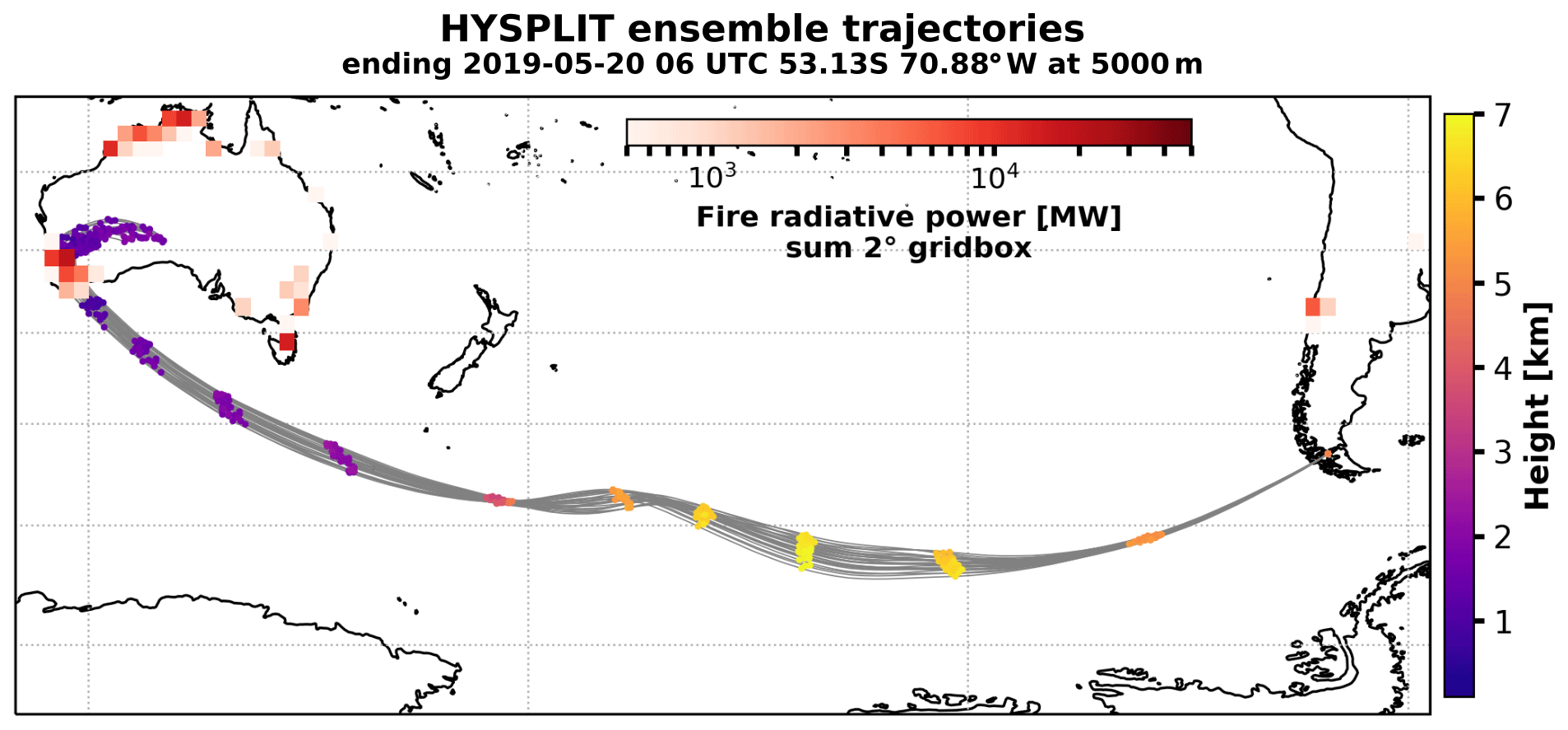
Figure A1HYSPLIT ensemble backward trajectories ending above Punta Arenas on 20 May 2019, 06:00 UTC, at 5 km height, together with the MODIS-derived fire radiative power (Giglio, 2000). Dots along the trajectories indicate the height of the air parcel in 12 h intervals. MODIS-derived fire radiative power of fires between 10 and 16 May 2019 is gridded to 2∘.
The processing software, as used for this publication, is available under https://doi.org/10.5281/zenodo.4438051 (Radenz, 2021). The most recent version is available via GitHub at https://github.com/martin-rdz/trace_airmass_source (last access: 14 January 2021). A Docker configuration is provided for a straightforward replication of the programming environment, including all dependencies. Meteorological fields for the backward simulations were obtained from https://www.ready.noaa.gov/gdas1.php (ARL Archive, 2019) and https://doi.org/10.5065/D6M043C6 (NCEP et al., 2000). The data for the fire radiative power map are available at https://doi.org/10.5067/FIRMS/MODIS/MCD14ML (Giglio, 2000). The analyzed PollyXT and air mass source data are available on request.
The supplement related to this article is available online at: https://doi.org/10.5194/acp-21-3015-2021-supplement.
MR developed the algorithm and drafted the paper. PS and JB supported the implementation and supervised the work. HB, AAF and ZY analyzed the lidar data. All authors jointly contributed to the paper and the scientific discussion.
The authors declare that they have no conflict of interest.
This article is part of the special issue “EARLINET aerosol profiling: contributions to atmospheric and climate research”. It is not associated with a conference.
We thank the Alfred Wegener Institute as well as the captain and crew of R/V Polarstern for their support (grant no. AWI_PS113_00). Many improvements to the Polly instruments, both in terms of hardware and software, were triggered by the fruitful discussions and network activities within EARLINET (Pappalardo et al., 2014). We thank Lucia Mona for serving as an editor and gratefully acknowledge the constructive comments from the two anonymous referees.
This research has been supported by the European Union's Horizon 2020 (ACTRIS; grant no. 654109), the Seventh Framework Programme (BACCHUS; grant no. 603445), the Federal Ministry of Education and Research in Germany (grant nos. 01LK1503F, 01LK1502I, 01LK1209C and 01LK1212C), the Alfred Wegener Institute Helmholtz Centre for Polar and Marine Research (grant no. AWI_PS113_00), and the German Federal Ministry for Economic Affairs and Energy (BMWi; grant no. 50EE1721C.
The publication of this article was funded by the
Open Access Fund of the Leibniz Association.
This paper was edited by Lucia Mona and reviewed by two anonymous referees.
Amiridis, V., Marinou, E., Tsekeri, A., Wandinger, U., Schwarz, A., Giannakaki, E., Mamouri, R., Kokkalis, P., Binietoglou, I., Solomos, S., Herekakis, T., Kazadzis, S., Gerasopoulos, E., Proestakis, E., Kottas, M., Balis, D., Papayannis, A., Kontoes, C., Kourtidis, K., Papagiannopoulos, N., Mona, L., Pappalardo, G., Le Rille, O., and Ansmann, A.: LIVAS: a 3-D multi-wavelength aerosol/cloud database based on CALIPSO and EARLINET, Atmos. Chem. Phys., 15, 7127–7153, https://doi.org/10.5194/acp-15-7127-2015, 2015. a
Ansmann, A., Mamouri, R.-E., Hofer, J., Baars, H., Althausen, D., and Abdullaev, S. F.: Dust mass, cloud condensation nuclei, and ice-nucleating particle profiling with polarization lidar: updated POLIPHON conversion factors from global AERONET analysis, Atmos. Meas. Tech., 12, 4849–4865, https://doi.org/10.5194/amt-12-4849-2019, 2019. a
Ansmann, A., Ohneiser, K., Mamouri, R.-E., Knopf, D. A., Veselovskii, I., Baars, H., Engelmann, R., Foth, A., Jimenez, C., Seifert, P., and Barja, B.: Tropospheric and stratospheric wildfire smoke profiling with lidar: Mass, surface area, CCN and INP retrieval, Atmos. Chem. Phys. Discuss. [preprint], https://doi.org/10.5194/acp-2020-1093, in review, 2020. a
ARL Archive: GDAS1 dataset, available at: https://www.ready.noaa.gov/gdas1.php, last access: 11 Novemer 2019. a, b
Ashbaugh, L. L.: A Statistical Trajectory Technique for Determining Air Pollution Source Regions, JAPCA J. Air Waste Ma., 33, 1096–1098, https://doi.org/10.1080/00022470.1983.10465702, 1983. a
Ashbaugh, L. L., Malm, W. C., and Sadeh, W. Z.: A residence time probability analysis of sulfur concentrations at grand Canyon National Park, Atmos. Environ., 19, 1263–1270, https://doi.org/10.1016/0004-6981(85)90256-2, 1985. a
Baars, H., Kanitz, T., Engelmann, R., Althausen, D., Heese, B., Komppula, M., Preißler, J., Tesche, M., Ansmann, A., Wandinger, U., Lim, J.-H., Ahn, J. Y., Stachlewska, I. S., Amiridis, V., Marinou, E., Seifert, P., Hofer, J., Skupin, A., Schneider, F., Bohlmann, S., Foth, A., Bley, S., Pfüller, A., Giannakaki, E., Lihavainen, H., Viisanen, Y., Hooda, R. K., Pereira, S. N., Bortoli, D., Wagner, F., Mattis, I., Janicka, L., Markowicz, K. M., Achtert, P., Artaxo, P., Pauliquevis, T., Souza, R. A. F., Sharma, V. P., van Zyl, P. G., Beukes, J. P., Sun, J., Rohwer, E. G., Deng, R., Mamouri, R.-E., and Zamorano, F.: An overview of the first decade of PollyNET: an emerging network of automated Raman-polarization lidars for continuous aerosol profiling, Atmos. Chem. Phys., 16, 5111–5137, https://doi.org/10.5194/acp-16-5111-2016, 2016. a, b, c, d, e, f, g, h
Baars, H., Seifert, P., Engelmann, R., and Wandinger, U.: Target categorization of aerosol and clouds by continuous multiwavelength-polarization lidar measurements, Atmos. Meas. Tech., 10, 3175–3201, https://doi.org/10.5194/amt-10-3175-2017, 2017. a, b, c
Baars, H., Ansmann, A., Ohneiser, K., Haarig, M., Engelmann, R., Althausen, D., Hanssen, I., Gausa, M., Pietruczuk, A., Szkop, A., Stachlewska, I. S., Wang, D., Reichardt, J., Skupin, A., Mattis, I., Trickl, T., Vogelmann, H., Navas-Guzmán, F., Haefele, A., Acheson, K., Ruth, A. A., Tatarov, B., Müller, D., Hu, Q., Podvin, T., Goloub, P., Veselovskii, I., Pietras, C., Haeffelin, M., Fréville, P., Sicard, M., Comerón, A., Fernández García, A. J., Molero Menéndez, F., Córdoba-Jabonero, C., Guerrero-Rascado, J. L., Alados-Arboledas, L., Bortoli, D., Costa, M. J., Dionisi, D., Liberti, G. L., Wang, X., Sannino, A., Papagiannopoulos, N., Boselli, A., Mona, L., D'Amico, G., Romano, S., Perrone, M. R., Belegante, L., Nicolae, D., Grigorov, I., Gialitaki, A., Amiridis, V., Soupiona, O., Papayannis, A., Mamouri, R.-E., Nisantzi, A., Heese, B., Hofer, J., Schechner, Y. Y., Wandinger, U., and Pappalardo, G.: The unprecedented 2017–2018 stratospheric smoke event: decay phase and aerosol properties observed with the EARLINET, Atmos. Chem. Phys., 19, 15183–15198, https://doi.org/10.5194/acp-19-15183-2019, 2019. a
Broxton, P. D., Zeng, X., Sulla-Menashe, D., and Troch, P. A.: A Global Land Cover Climatology Using MODIS Data, J. Appl. Meteorol. Climatol., 53, 1593–1605, https://doi.org/10.1175/JAMC-D-13-0270.1, 2014. a, b
Burton, S. P., Ferrare, R. A., Hostetler, C. A., Hair, J. W., Rogers, R. R., Obland, M. D., Butler, C. F., Cook, A. L., Harper, D. B., and Froyd, K. D.: Aerosol classification using airborne High Spectral Resolution Lidar measurements – methodology and examples, Atmos. Meas. Tech., 5, 73–98, https://doi.org/10.5194/amt-5-73-2012, 2012. a
D'Amico, G., Amodeo, A., Baars, H., Binietoglou, I., Freudenthaler, V., Mattis, I., Wandinger, U., and Pappalardo, G.: EARLINET Single Calculus Chain – overview on methodology and strategy, Atmos. Meas. Tech., 8, 4891–4916, https://doi.org/10.5194/amt-8-4891-2015, 2015. a
Dipu, S., Quaas, J., Wolke, R., Stoll, J., Mühlbauer, A., Sourdeval, O., Salzmann, M., Heinold, B., and Tegen, I.: Implementation of aerosol–cloud interactions in the regional atmosphere–aerosol model COSMO-MUSCAT(5.0) and evaluation using satellite data, Geosci. Model Dev., 10, 2231–2246, https://doi.org/10.5194/gmd-10-2231-2017, 2017. a
Draxler, R. R.: Evaluation of an Ensemble Dispersion Calculation, J. Appl. Meteorol., 42, 308–317, https://doi.org/10.1175/1520-0450(2003)042<0308:EOAEDC>2.0.CO;2, 2003. a
Engelmann, R., Kanitz, T., Baars, H., Heese, B., Althausen, D., Skupin, A., Wandinger, U., Komppula, M., Stachlewska, I. S., Amiridis, V., Marinou, E., Mattis, I., Linné, H., and Ansmann, A.: The automated multiwavelength Raman polarization and water-vapor lidar PollyXT: the neXT generation, Atmos. Meas. Tech., 9, 1767–1784, https://doi.org/10.5194/amt-9-1767-2016, 2016. a
Escudero, M., Stein, A., Draxler, R., Querol, X., Alastuey, A., Castillo, S., and Avila, A.: Source apportionment for African dust outbreaks over the Western Mediterranean using the HYSPLIT model, Atmos. Res., 99, 518–527, https://doi.org/10.1016/j.atmosres.2010.12.002, 2011. a
Feuerstein, S. and Schepanski, K.: Identification of Dust Sources in a Saharan Dust Hot-Spot and Their Implementation in a Dust-Emission Model, Remote Sens., 11, 4, https://doi.org/10.3390/rs11010004, 2018. a
Fleming, Z. L., Monks, P. S., and Manning, A. J.: Review: Untangling the influence of air-mass history in interpreting observed atmospheric composition, Atmos. Res., 104–105, 1–39, https://doi.org/10.1016/j.atmosres.2011.09.009, 2012. a
Flemming, J., Benedetti, A., Inness, A., Engelen, R. J., Jones, L., Huijnen, V., Remy, S., Parrington, M., Suttie, M., Bozzo, A., Peuch, V.-H., Akritidis, D., and Katragkou, E.: The CAMS interim Reanalysis of Carbon Monoxide, Ozone and Aerosol for 2003–2015, Atmos. Chem. Phys., 17, 1945–1983, https://doi.org/10.5194/acp-17-1945-2017, 2017. a
Floutsi, A. A., Baars, H., Radenz, M., Haarig, M., Yin, Z., Seifert, P., Jimenez, C., Ansmann, A., Engelmann, R., Barja, B., Zamorano, F., and Wandinger, U.: Advection of Biomass Burning Aerosols towards the Southern Hemispheric Mid-Latitude Station of Punta Arenas as Observed with Multiwavelength Polarization Raman Lidar, Remote Sens., 13, 138, https://doi.org/10.3390/rs13010138, 2021. a, b
Foth, A., Kanitz, T., Engelmann, R., Baars, H., Radenz, M., Seifert, P., Barja, B., Fromm, M., Kalesse, H., and Ansmann, A.: Vertical aerosol distribution in the southern hemispheric midlatitudes as observed with lidar in Punta Arenas, Chile (53.2∘ S and 70.9∘ W), during ALPACA, Atmos. Chem. Phys., 19, 6217–6233, https://doi.org/10.5194/acp-19-6217-2019, 2019. a, b
Friedl, M., McIver, D., Hodges, J., Zhang, X., Muchoney, D., Strahler, A., Woodcock, C., Gopal, S., Schneider, A., Cooper, A., Baccini, A., Gao, F., and Schaaf, C.: Global land cover mapping from MODIS: algorithms and early results, Remote Sensing of Environment, 83, 287–302, https://doi.org/10.1016/S0034-4257(02)00078-0, 2002. a
Giglio, L.: MODIS Thermal Anomalies/Fire Products, NASA Earth Observing System Data and Information System (EOSDIS), https://doi.org/10.5067/FIRMS/MODIS/MCD14ML, 2000. a, b
Groß, S., Esselborn, M., Weinzierl, B., Wirth, M., Fix, A., and Petzold, A.: Aerosol classification by airborne high spectral resolution lidar observations, Atmos. Chem. Phys., 13, 2487–2505, https://doi.org/10.5194/acp-13-2487-2013, 2013. a
Haarig, M., Ansmann, A., Gasteiger, J., Kandler, K., Althausen, D., Baars, H., Radenz, M., and Farrell, D. A.: Dry versus wet marine particle optical properties: RH dependence of depolarization ratio, backscatter, and extinction from multiwavelength lidar measurements during SALTRACE, Atmos. Chem. Phys., 17, 14199–14217, https://doi.org/10.5194/acp-17-14199-2017, 2017. a
Hamilton, D. S., Lee, L. A., Pringle, K. J., Reddington, C. L., Spracklen, D. V., and Carslaw, K. S.: Occurrence of pristine aerosol environments on a polluted planet, P. Natl. Acad. Sci., 111, 18466–18471, https://doi.org/10.1073/pnas.1415440111, 2014. a
Heintzenberg, J., Birmili, W., Seifert, P., Panov, A., Chi, X., and Andreae, M. O.: Mapping the aerosol over Eurasia from the Zotino Tall Tower, Tellus B, 65, 20062, https://doi.org/10.3402/tellusb.v65i0.20062, 2013. a
Illingworth, A. J., Hogan, R. J., O'Connor, E. J., Bouniol, D., Delanoë, J., Pelon, J., Protat, A., Brooks, M. E., Gaussiat, N., Wilson, D. R., Donovan, D. P., Baltink, H. K., van Zadelhoff, G.-J., Eastment, J. D., Goddard, J. W. F., Wrench, C. L., Haeffelin, M., Krasnov, O. A., Russchenberg, H. W. J., Piriou, J.-M., Vinit, F., Seifert, A., Tompkins, A. M., and Willén, U.: Cloudnet: Continuous Evaluation of Cloud Profiles in Seven Operational Models Using Ground-Based Observations, B. Am. Meteorol. Soc., 88, 883–898, https://doi.org/10.1175/BAMS-88-6-883, 2007. a
Illingworth, A. J., Barker, H. W., Beljaars, A., Ceccaldi, M., Chepfer, H., Clerbaux, N., Cole, J., Delanoë, J., Domenech, C., Donovan, D. P., Fukuda, S., Hirakata, M., Hogan, R. J., Huenerbein, A., Kollias, P., Kubota, T., Nakajima, T., Nakajima, T. Y., Nishizawa, T., Ohno, Y., Okamoto, H., Oki, R., Sato, K., Satoh, M., Shephard, M. W., Velázquez-Blázquez, A., Wandinger, U., Wehr, T., and van Zadelhoff, G.-J.: The EarthCARE Satellite: The Next Step Forward in Global Measurements of Clouds, Aerosols, Precipitation, and Radiation, B. Am. Meteor. Soc., 96, 1311–1332, https://doi.org/10.1175/BAMS-D-12-00227.1, 2015. a, b
Kahl, J. D.: A cautionary note on the use of air trajectories in interpreting atmospheric chemistry measurements, Atmos. Environ., 27, 3037–3038, https://doi.org/10.1016/0960-1686(93)90336-W, 1993. a
Lu, Z., Streets, D. G., Zhang, Q., and Wang, S.: A novel back-trajectory analysis of the origin of black carbon transported to the Himalayas and Tibetan Plateau during 1996–2010, Geophys. Res. Lett., 39, L01809, https://doi.org/10.1029/2011GL049903, 2012. a
Mamouri, R. E., Ansmann, A., Nisantzi, A., Kokkalis, P., Schwarz, A., and Hadjimitsis, D.: Low Arabian dust extinction-to-backscatter ratio, Geophys. Res. Lett., 40, 4762–4766, https://doi.org/10.1002/grl.50898, 2013. a
Matthias, V., Balis, D., Bösenberg, J., Eixmann, R., Iarlori, M., Komguem, L., Mattis, I., Papayannis, A., Pappalardo, G., Perrone, M. R., and Wang, X.: Vertical aerosol distribution over Europe: Statistical analysis of Raman lidar data from 10 European Aerosol Research Lidar Network (EARLINET) stations, J. Geophys. Res.-Atmos., 109, D18201, https://doi.org/10.1029/2004JD004638, 2004. a
Mattis, I., Müller, D., Ansmann, A., Wandinger, U., Preißler, J., Seifert, P., and Tesche, M.: Ten years of multiwavelength Raman lidar observations of free-tropospheric aerosol layers over central Europe: Geometrical properties and annual cycle, J. Geophys. Res.-Atmos., 113, D20202, https://doi.org/10.1029/2007JD009636, 2008. a
Merrill, J. T., Bleck, R., and Avila, L.: Modeling atmospheric transport to the Marshall Islands, J. Geophys. Res.-Atmos., 90, 12927–12936, https://doi.org/10.1029/JD090iD07p12927, 1985. a
Müller, D., Ansmann, A., Mattis, I., Tesche, M., Wandinger, U., Althausen, D., and Pisani, G.: Aerosol-type-dependent lidar ratios observed with Raman lidar, J. Geophys. Res.-Atmos., 112, D16202, https://doi.org/10.1029/2006JD008292, 2007. a
Mylonaki, M., Giannakaki, E., Papayannis, A., Papanikolaou, C.-A., Komppula, M., Nicolae, D., Papagiannopoulos, N., Amodeo, A., Baars, H., and Soupiona, O.: Aerosol type classification analysis using EARLINET multiwavelength and depolarization lidar observations, Atmos. Chem. Phys. Discuss. [preprint], https://doi.org/10.5194/acp-2020-865, in review, 2020. a
Nicolae, D., Vasilescu, J., Talianu, C., Binietoglou, I., Nicolae, V., Andrei, S., and Antonescu, B.: A neural network aerosol-typing algorithm based on lidar data, Atmos. Chem. Phys., 18, 14511–14537, https://doi.org/10.5194/acp-18-14511-2018, 2018. a
Nisantzi, A., Mamouri, R. E., Ansmann, A., Schuster, G. L., and Hadjimitsis, D. G.: Middle East versus Saharan dust extinction-to-backscatter ratios, Atmos. Chem. Phys., 15, 7071–7084, https://doi.org/10.5194/acp-15-7071-2015, 2015. a
National Centers For Environmental Prediction/National Weather Service/NOAA/U.S. Department Of Commerce: NCEP FNL Operational Model Global Tropospheric Analyses continuing from July 1999, UCAR/NCAR – Research Data Archive, https://doi.org/10.5065/D6M043C6, 2000. a, b
Papagiannopoulos, N., D'Amico, G., Gialitaki, A., Ajtai, N., Alados-Arboledas, L., Amodeo, A., Amiridis, V., Baars, H., Balis, D., Binietoglou, I., Comerón, A., Dionisi, D., Falconieri, A., Fréville, P., Kampouri, A., Mattis, I., Mijić, Z., Molero, F., Papayannis, A., Pappalardo, G., Rodríguez-Gómez, A., Solomos, S., and Mona, L.: An EARLINET early warning system for atmospheric aerosol aviation hazards, Atmos. Chem. Phys., 20, 10775–10789, https://doi.org/10.5194/acp-20-10775-2020, 2020. a, b
Pappalardo, G., Mona, L., D'Amico, G., Wandinger, U., Adam, M., Amodeo, A., Ansmann, A., Apituley, A., Alados Arboledas, L., Balis, D., Boselli, A., Bravo-Aranda, J. A., Chaikovsky, A., Comeron, A., Cuesta, J., De Tomasi, F., Freudenthaler, V., Gausa, M., Giannakaki, E., Giehl, H., Giunta, A., Grigorov, I., Groß, S., Haeffelin, M., Hiebsch, A., Iarlori, M., Lange, D., Linné, H., Madonna, F., Mattis, I., Mamouri, R.-E., McAuliffe, M. A. P., Mitev, V., Molero, F., Navas-Guzman, F., Nicolae, D., Papayannis, A., Perrone, M. R., Pietras, C., Pietruczuk, A., Pisani, G., Preißler, J., Pujadas, M., Rizi, V., Ruth, A. A., Schmidt, J., Schnell, F., Seifert, P., Serikov, I., Sicard, M., Simeonov, V., Spinelli, N., Stebel, K., Tesche, M., Trickl, T., Wang, X., Wagner, F., Wiegner, M., and Wilson, K. M.: Four-dimensional distribution of the 2010 Eyjafjallajökull volcanic cloud over Europe observed by EARLINET, Atmos. Chem. Phys., 13, 4429–4450, https://doi.org/10.5194/acp-13-4429-2013, 2013. a
Pappalardo, G., Amodeo, A., Apituley, A., Comeron, A., Freudenthaler, V., Linné, H., Ansmann, A., Bösenberg, J., D'Amico, G., Mattis, I., Mona, L., Wandinger, U., Amiridis, V., Alados-Arboledas, L., Nicolae, D., and Wiegner, M.: EARLINET: towards an advanced sustainable European aerosol lidar network, Atmos. Meas. Tech., 7, 2389–2409, https://doi.org/10.5194/amt-7-2389-2014, 2014. a, b, c
Paris, J.-D., Stohl, A., Ciais, P., Nédélec, P., Belan, B. D., Arshinov, M. Yu., and Ramonet, M.: Source-receptor relationships for airborne measurements of CO2, CO and O3 above Siberia: a cluster-based approach, Atmos. Chem. Phys., 10, 1671–1687, https://doi.org/10.5194/acp-10-1671-2010, 2010. a
Pisso, I., Sollum, E., Grythe, H., Kristiansen, N. I., Cassiani, M., Eckhardt, S., Arnold, D., Morton, D., Thompson, R. L., Groot Zwaaftink, C. D., Evangeliou, N., Sodemann, H., Haimberger, L., Henne, S., Brunner, D., Burkhart, J. F., Fouilloux, A., Brioude, J., Philipp, A., Seibert, P., and Stohl, A.: The Lagrangian particle dispersion model FLEXPART version 10.4, Geosci. Model Dev., 12, 4955–4997, https://doi.org/10.5194/gmd-12-4955-2019, 2019. a, b, c
Polissar, A., Hopke, P., Paatero, P., Kaufmann, Y., Hall, D., Bodhaine, B., Dutton, E., and Harris, J.: The aerosol at Barrow, Alaska: long-term trends and source locations, Atmos. Environ., 33, 2441–2458, https://doi.org/10.1016/S1352-2310(98)00423-3, 1999. a
Radenz, M.: martin-rdz/trace_airmass_source: trace_airmass_source jan2021, Zenodo, https://doi.org/10.5281/zenodo.4438051, 2021. a
Reitebuch, O.: The Spaceborne Wind Lidar Mission ADM-Aeolus, Springer Berlin Heidelberg, Berlin, Heidelberg, 815–827, https://doi.org/10.1007/978-3-642-30183-4_49, 2012. a
Rieger, D., Bangert, M., Bischoff-Gauss, I., Förstner, J., Lundgren, K., Reinert, D., Schröter, J., Vogel, H., Zängl, G., Ruhnke, R., and Vogel, B.: ICON–ART 1.0 – a new online-coupled model system from the global to regional scale, Geosci. Model Dev., 8, 1659–1676, https://doi.org/10.5194/gmd-8-1659-2015, 2015. a
Rittmeister, F., Ansmann, A., Engelmann, R., Skupin, A., Baars, H., Kanitz, T., and Kinne, S.: Profiling of Saharan dust from the Caribbean to western Africa – Part 1: Layering structures and optical properties from shipborne polarization/Raman lidar observations, Atmos. Chem. Phys., 17, 12963–12983, https://doi.org/10.5194/acp-17-12963-2017, 2017. a
Seibert, P.: Convergence and Accuracy of Numerical Methods for Trajectory Calculations, J. Appl. Meteorol., 32, 558–566, https://doi.org/10.1175/1520-0450(1993)032<0558:CAAONM>2.0.CO;2, 1993. a
Stein, A. F., Draxler, R. R., Rolph, G. D., Stunder, B. J. B., Cohen, M. D., and Ngan, F.: NOAA’s HYSPLIT Atmospheric Transport and Dispersion Modeling System, B. Am. Meteorol. Soc., 96, 2059–2077, https://doi.org/10.1175/BAMS-D-14-00110.1, 2015. a, b
Stohl, A.: Trajectory statistics-A new method to establish source-receptor relationships of air pollutants and its application to the transport of particulate sulfate in Europe, Atmos. Environ., 30, 579–587, https://doi.org/10.1016/1352-2310(95)00314-2, 1996. a
Stohl, A.: Computation, accuracy and applications of trajectories–A review and bibliography, Atmos. Environ., 32, 947–966, https://doi.org/10.1016/S1352-2310(97)00457-3, 1998. a
Stohl, A., Wotawa, G., Seibert, P., and Kromp-Kolb, H.: Interpolation Errors in Wind Fields as a Function of Spatial and Temporal Resolution and Their Impact on Different Types of Kinematic Trajectories, J. Appl. Meteorol., 34, 2149–2165, https://doi.org/10.1175/1520-0450(1995)034<2149:IEIWFA>2.0.CO;2, 1995. a
Stohl, A., Eckhardt, S., Forster, C., James, P., Spichtinger, N., and Seibert, P.: A replacement for simple back trajectory calculations in the interpretation of atmospheric trace substance measurements, Atmos. Environ., 36, 4635–4648, https://doi.org/10.1016/S1352-2310(02)00416-8, 2002. a
Stohl, A., Forster, C., Frank, A., Seibert, P., and Wotawa, G.: Technical note: The Lagrangian particle dispersion model FLEXPART version 6.2, Atmos. Chem. Phys., 5, 2461–2474, https://doi.org/10.5194/acp-5-2461-2005, 2005. a
Strass, V. H.: The Expedition PS113 of the Research Vessel POLARSTERN to the Atlantic Ocean in 2018, Reports on Polar and Marine Research, Alfred-Wegener-Institut, Helmholtz-Zentrum für Polar- und Meeresforschung, Bremerhaven, Germany, 724, 1–66, https://doi.org/10.2312/BzPM_0724_2018, 2018. a
Tarasova, O. A., Senik, I. A., Sosonkin, M. G., Cui, J., Staehelin, J., and Prévôt, A. S. H.: Surface ozone at the Caucasian site Kislovodsk High Mountain Station and the Swiss Alpine site Jungfraujoch: data analysis and trends (1990–2006), Atmos. Chem. Phys., 9, 4157–4175, https://doi.org/10.5194/acp-9-4157-2009, 2009. a
Tesche, M., Ansmann, A., Müller, D., Althausen, D., Engelmann, R., Freudenthaler, V., and Groß, S.: Vertically resolved separation of dust and smoke over Cape Verde using multiwavelength Raman and polarization lidars during Saharan Mineral Dust Experiment 2008, J. Geophys. Res.-Atmos., 114, D13202, https://doi.org/10.1029/2009JD011862, 2009. a
Tesche, M., Gross, S., Ansmann, A., Müller, D., Althausen, D., Freudenthaler, V., and Esselborn, M.: Profiling of Saharan dust and biomass-burning smoke with multiwavelength polarization Raman lidar at Cape Verde, Tellus B, 63, 649–676, https://doi.org/10.1111/j.1600-0889.2011.00548.x, 2011. a
Val Martin, M., Kahn, R., and Tosca, M.: A Global Analysis of Wildfire Smoke Injection Heights Derived from Space-Based Multi-Angle Imaging, Remote Sens., 10, 1609, https://doi.org/10.3390/rs10101609, 2018. a, b, c
Veselovskii, I., Whiteman, D. N., Korenskiy, M., Suvorina, A., Kolgotin, A., Lyapustin, A., Wang, Y., Chin, M., Bian, H., Kucsera, T. L., Pérez-Ramírez, D., and Holben, B.: Characterization of forest fire smoke event near Washington, DC in summer 2013 with multi-wavelength lidar, Atmos. Chem. Phys., 15, 1647–1660, https://doi.org/10.5194/acp-15-1647-2015, 2015. a
Veselovskii, I., Goloub, P., Podvin, T., Bovchaliuk, V., Tanre, D., Derimian, Y., Korenskiy, M., and Dubovik, O.: Study of African Dust with Multi-Wavelength Raman Lidar During “Shadow” Campaign in Senegal, EPJ Web of Conferences, 119, 08003, https://doi.org/10.1051/epjconf/201611908003, 2016. a
Wandinger, U., Baars, H., Engelmann, R., Hünerbein, A., Horn, S., Kanitz, T., Donovan, D., van Zadelhoff, G.-J., Daou, D., Fischer, J., von Bismarck, J., Filipitsch, F., Docter, N., Eisinger, M., Lajas, D., and Wehr, T.: HETEAC: The Aerosol Classification Model for EarthCARE, EPJ Web of Conferences, 119, 01004, https://doi.org/10.1051/epjconf/201611901004, 2016. a
Wernli, B. H. and Davies, H. C.: A lagrangian-based analysis of extratropical cyclones. I: The method and some applications, Q. J. Roy. Meteorol. Soc., 123, 467–489, https://doi.org/10.1002/qj.49712353811, 1997. a
Winker, D. M., Vaughan, M. A., Omar, A., Hu, Y., Powell, K. A., Liu, Z., Hunt, W. H., and Young, S. A.: Overview of the CALIPSO Mission and CALIOP Data Processing Algorithms, J. Atmos. Ocean. Tech., 26, 2310–2323, https://doi.org/10.1175/2009jtecha1281.1, 2009. a
Winker, D. M., Tackett, J. L., Getzewich, B. J., Liu, Z., Vaughan, M. A., and Rogers, R. R.: The global 3-D distribution of tropospheric aerosols as characterized by CALIOP, Atmos. Chem. Phys., 13, 3345–3361, https://doi.org/10.5194/acp-13-3345-2013, 2013. a
Yin, Z. and Baars, H.: PollyNET/Pollynet_Processing_Chain: Version 2.0, Zenodo, https://doi.org/10.5281/zenodo.3774689, 2020. a
Yin, Z., Ansmann, A., Baars, H., Seifert, P., Engelmann, R., Radenz, M., Jimenez, C., Herzog, A., Ohneiser, K., Hanbuch, K., Blarel, L., Goloub, P., Dubois, G., Victori, S., and Maupin, F.: Aerosol measurements with a shipborne Sun–sky–lunar photometer and collocated multiwavelength Raman polarization lidar over the Atlantic Ocean, Atmos. Meas. Tech., 12, 5685–5698, https://doi.org/10.5194/amt-12-5685-2019, 2019. a, b, c, d
- Abstract
- Introduction
- Air mass source attribution method
- PollyXT lidar observations
- Application to lidar case studies
- Assessing potential observation biases
- Discussion and conclusions
- Appendix A
- Code and data availability
- Author contributions
- Competing interests
- Special issue statement
- Acknowledgements
- Financial support
- Review statement
- References
- Supplement