the Creative Commons Attribution 4.0 License.
the Creative Commons Attribution 4.0 License.
 | 15 Feb 2021
Aerosol type classification analysis using EARLINET multiwavelength and depolarization lidar observations
Elina Giannakaki
Alexandros Papayannis
Christina-Anna Papanikolaou
Mika Komppula
Doina Nicolae
Nikolaos Papagiannopoulos
Aldo Amodeo
Holger Baars
Ourania Soupiona
We introduce an automated aerosol type classification method, called Source Classification Analysis (SCAN). SCAN is based on predefined and characterized aerosol source regions, the time that the air parcel spends above each geographical region, and a number of additional criteria. The output of SCAN is compared with two independent aerosol classification methods, which use the intensive optical parameters from lidar data: (1) the Mahalanobis distance automatic aerosol type classification (MD) and (2) a neural network aerosol typing algorithm (NATALI). In this paper, data from the European Aerosol Research Lidar Network (EARLINET) have been used. A total of 97 free tropospheric aerosol layers from four typical EARLINET stations (i.e., Bucharest, Kuopio, Leipzig, and Potenza) in the period 2014–2018 were classified based on a lidar configuration. We found that SCAN, as a method independent of optical properties, is not affected by overlapping optical values of different aerosol types. Furthermore, SCAN has no limitations concerning its ability to classify different aerosol mixtures. Additionally, it is a valuable tool to classify aerosol layers based on even single (elastic) lidar signals in the case of lidar stations that cannot provide a full data set () of aerosol optical properties; therefore, it can work independently of the capabilities of a lidar system. Finally, our results show that NATALI has a lower percentage of unclassified layers (4 %), while MD has a higher percentage of unclassified layers (50 %) and a lower percentage of cases classified as aerosol mixtures (5 %).


Aerosol particles directly affect the Earth's radiation budget by interacting mainly with solar radiation through absorption and scattering (aerosol–radiation interaction – ARI) (Hobbs, 1993). Furthermore, aerosols affect cloud formation and behavior, not only serving as seeds (cloud condensation nuclei, ice nuclei) upon which cloud droplets and ice crystals form, but also influencing the cloud albedo due to changing concentrations of cloud condensation and ice nuclei, also known as the Twomey effect (Twomey, 1959; Boucher et al., 2013; Rosenfeld et al., 2014, 2016).
The light detection and ranging (lidar) technique, which is based on the active remote sensing of the atmosphere (Weitcamp et al., 2005), has received quite a lot of attention because of the multiple possibilities to retrieve near-real-time information on the vertical structure and the composition of the atmosphere with high spatial (i.e., down to a few meters) and temporal (i.e., down to seconds depending on the system) resolution. Specifically, multiwavelength Raman and depolarization lidars can be used for aerosol detection and characterization (i.e., dust, smoke, continental). They can provide vertically resolved information on extensive and intensive aerosol optical properties (Freudenthaler et al., 2009; Nicolae et al., 2006; Burton et al., 2012; Groß et al., 2013; Giannakaki et al., 2016; Soupiona et al., 2018, 2019). These properties are the particle backscatter (bλα) and extinction coefficients (eλα), the lidar ratio (LRλα), the Ångström exponent extinction () and backscatter (), and the particle linear depolarization ratio (PLDR). Towards this direction, the large majority of European Aerosol Research Lidar Network (EARLINET) stations use multiwavelength Raman lidar systems that combine detection channels at both elastic and Raman-shifted signals and are equipped with depolarization channels (Pappalardo et al., 2014).
Until recently, the identification of aerosol layers was based, apart from aerosol lidar data, on air-mass back-trajectory analysis, atmospheric models (e.g., DREAM; Basart et al., 2012), concurrent satellite products (MODIS dust and fire data; e.g., Giglio et al., 2013), and ground-based photometric data (Papayannis et al., 2005, 2008). It is well-established that air-mass trajectory analysis (back to several hours) with the HYSPLIT (Draxler et al., 2013) or FLEXPART (FLEXible PARTicle dispersion model; Stohl et al., 2005) models ending above the observation station is used in order to identify the air-mass origin of the detected layer. However, this case-by-case aerosol layer identification is neither objective nor automated.
To overcome this defect, two automated methods have been developed recently to classify aerosol layers observed by lidars: (1) the Mahalanobis distance aerosol classification algorithm (MD) (Papagiannopoulos et al., 2018), which uses lidar intensive properties (LRλα, the lidar ratio – LRλ1 LRλ2, , , and PLDR if provided) in order to classify the measured aerosol layers into a number of aerosol types, and (2) a neural network aerosol classification algorithm (NATALI) (Nicolae et al., 2018a), which is based on artificial neural networks (ANNs) trained to estimate the most probable aerosol type solely from a set of multispectral lidar data (color index – CI, color ratio – CR, LRλα, , , and PLDR if provided). In reality, intensive aerosol optical properties can vary greatly even for single aerosol types. For example, Nicolae et al. (2013) showed that fresh biomass burning aerosols have higher Ångström exponents and refractive indexes than aged ones. Additionally, according to Veselovkii et al. (2020), the lidar ratio values of dust aerosols can vary greatly depending on the source region mineralogy. Thus, the physicochemical modifications the aerosols undergo, from the time they are created to when they are finally observed, change their geometrical, size, and optical characteristics. As a result, their optical properties change as well. Taking into account that both NATALI and MD experience several limitations, as they request as input the aerosol intensive optical properties as stated previously (Nicolae et al., 2018b; Voudouri et al., 2019), a more generic aerosol classification code free from these defects is needed.
Therefore, in this work, we develop an improved automated layer classification algorithm based on air-mass backward-trajectory analysis and satellite data. The algorithm, called Source Classification Analysis (SCAN), is based on the amount of time that the air parcel spends above an already characterized aerosol source region and a number of additional criteria. This algorithm, being independent of aerosol optical properties, provides the advantage that its classification process is not affected by overlapping values of optical properties representing more than one aerosol type (e.g., clean continental, continental polluted, smoke). Furthermore, it has no limitations concerning its ability to classify aerosol mixtures. Finally, it can be useful for all types of lidar systems (independently of the number of channels used) and for other network-based systems (radar profilers, sun photometers).
In this paper, we use SCAN, MD, and NATALI as classifiers to assign lidar observations to the pre-specified aerosol classes. The three different aerosol classification methods are described in Sect. 2, while Sect. 3 provides a discussion of the results and a comparison between them. Finally, Sect. 4 provides the conclusions of our study.
2.1 Aerosol layer classification algorithms
2.1.1 Neural network aerosol classification algorithm
NATALI (Nicolae et al., 2018a) is an automated, optical-property-dependent aerosol layer classification algorithm. The typical aerosol profiles ( PLDR, optional; in NetCDF format) from the EARLINET database are used as inputs in order to retrieve the mean aerosol optical properties within the layer boundaries indicated by the gradient method (Belegante et al., 2014). The learning process of the ANN has been performed using a synthetic database developed by Koepke et al. (1997) along with the T-matrix numerical method (Waterman, 1971; Mishchenko et al., 1996) to iteratively compute the intensive optical properties of six pure aerosol types (the first six aerosol types in Table 1) presented to the artificial neural networks to perform the typing. The synthetic database is built for 350, 550, and 1000 nm wavelengths, which are then rescaled to the usual lidar wavelengths (i.e., 355, 532, and 1064 nm) using an Ångström exponent equal to 1. The mixtures are obtained through a linear combination of pure aerosol properties (Nicolae et al., 2018a).
Two classification schemes are used with different aerosol type (classification) resolutions when particle depolarization data are available. The first one is applied when all the high-quality aerosol optical parameters are provided (uncertainty of eλα≤50 %, uncertainty of bλα≤20 %, uncertainty of PLDR ≤30 %) and the aerosol typing is performed in the high-resolution (AH) mode. This means that the aerosol mixtures can be sufficiently resolved, providing the maximum number of output types (14 types, Table 1). In the second scheme, the values of the aerosol optical parameters have high uncertainty (uncertainty of eλα>50 %, uncertainty of bλα>20 %, uncertainty of the PLDR >30 %), and the typing is performed in the low-resolution (AL) mode. In this case, the number of output types is limited to six (first six aerosol types; Table 1). A “voting” procedure selects the most probable answer out of the two (possibly different) individual returns. The correct answer is selected based on a statistical approach considering two criteria: (i) which answer has a higher confidence and (ii) which answer is more stable over the uncertainty range (i.e., the percentage of agreement for values between error limits). Finally, there is the capability to perform the typing when the particle depolarization is not available, knowing that the mixtures cannot be resolved, so only the predominant aerosol type is retrieved (Nicolae et al., 2018a).
2.1.2 Mahalanobis distance aerosol classification algorithm
The automatic classification algorithm described in Papagiannopoulos et al. (2018) makes use of the Mahalanobis distance function (Mahalanobis, 1936) that relates an unclassified measurement to a predefined aerosol type. The method compares observations to model distributions that comprise EARLINET pre-classified data. Each Mahalanobis distance of an observation from a specific aerosol type is estimated, and the aerosol type is assigned for the minimum distance. Prior to the classification, two screening criteria are assumed to ensure correct classification. The algorithm is able to classify an observation to a maximum of eight (dust, volcanic, mixed dust, polluted dust, clean continental, mixed marine, polluted continental, and smoke) and minimum of four (dust + volcanic + mixed dust + polluted dust, mixed marine, smoke + polluted continental, and clean continental) aerosol classes depending on the lidar configuration.
In this study, we used four aerosol intensive properties: the backscatter-related Ångström exponent at 355 and 1064 nm, the aerosol lidar ratio at 532 nm, the color ratio of the lidar ratios, and the aerosol particle linear depolarization ratio at 532 nm, while the minimum accepted distance was set to 4.3 (Papagiannopoulos et al., 2018). As soon as the distance from a specific aerosol class is below the threshold and the remaining distances are higher than the threshold, the observation is assigned to that aerosol class. If more than one distance is below the threshold, the normalized probability of each class needs to be over 50 %.
This objective multidimensional classification scheme has found great applicability and has been used with lidar (e.g., Burton et al., 2012; Papagiannopoulos et al., 2018), space-based polarimetry (Russell et al., 2014), and spectral photometry (e.g., Hamill et al., 2020; Siomos et al., 2020) data. Voudouri et al. (2019) compared NATALI and the Mahalanobis distance classification algorithm for the EARLINET station in Thessaloniki. Their study used a 3bλα+2eλα lidar configuration and four aerosol classes (i.e., dust, maritime, polluted smoke, and clean continental) for each automatic algorithm. In general, they found fair agreement between MD and NATALI, and the differences were attributed to the class definition and the range of the class intensive properties.
2.1.3 Source Classification Analysis
SCAN is an automated aerosol layer classification process that is independent of optical properties and has been developed in the IDL programming language in the framework of this study. For each identified aerosol layer an X h HYSPLIT backward trajectory (Draxler et al., 2013) is used to calculate the amount of time traveled above predefined aerosol source regions before arriving over a lidar station at the specific date and height that the aerosol layer is observed. X is the number of hours of the backward trajectory, which can be decided by the user at the beginning of the process. SCAN assumes specific regions (Fig. 1, colored squares; from now on referred to as domains) in terms of aerosol sources (Penning de Vries et al., 2015). The polluted continental domains represent the regions with increased anthropogenic activity according to monthly means of tropospheric NO2 from GOME-2 (Georgloulias et al., 2019).
Taking into account the information (latitude, longitude and height) from each HYSPLIT air-mass backward trajectory, SCAN implements a number of criteria: (i) if the geographical coordinates for the specific hour of the backward trajectory are within the boundaries of the marine domains and if the height of this trajectory over the domain is below 1 km (Wu et al., 2008; Ho et al., 2015), SCAN assigns this layer to the marine aerosol type. (ii) If the geographical coordinates for the specific hour of the backward trajectory are within the boundaries of the clean continental, polluted continental, or dust domains and if the height of this backward trajectory is below 2 km over the domain, SCAN assigns the specific hour to the clean continental, polluted continental, or dust aerosol type, respectively. (iii) For an hour to be assigned to the smoke aerosol type, except from the coordinates of the backward trajectory at this specific hour, which should be within the boundaries of the clean continental or polluted continental domains, the height of the trajectory at this specific hour should be below 3 km (Amiridis et al., 2010).
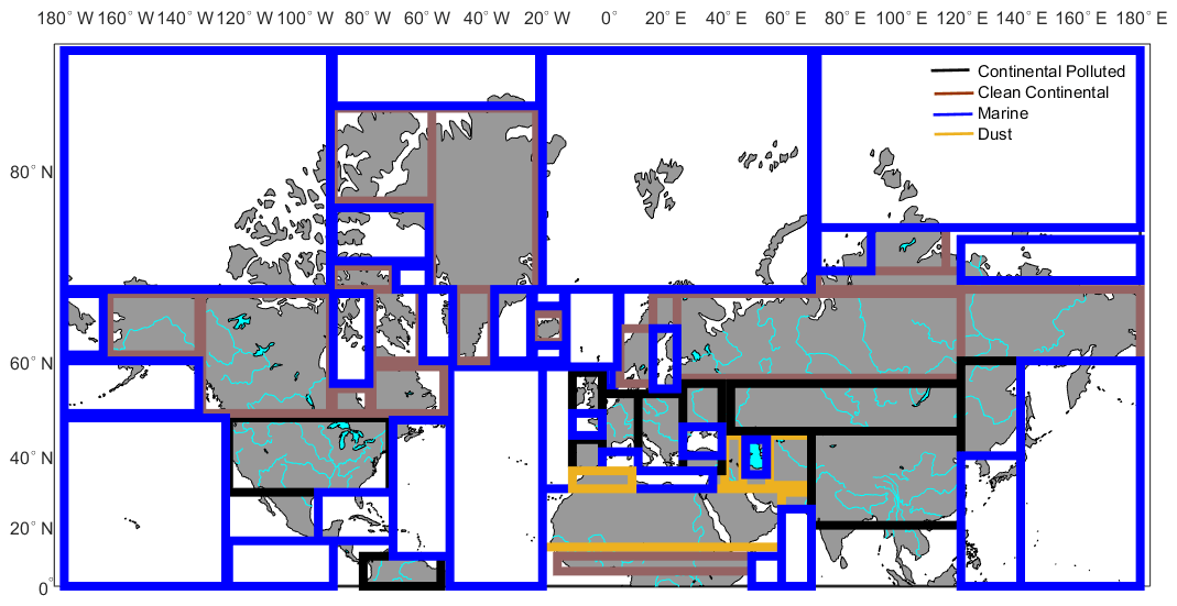
Figure 1SCAN's aerosol source type classification map. Different colored squares represent different aerosol sources: orange squares correspond to dust, blue squares to marine, brown squares to clean continental, and black squares to continental polluted aerosol sources.
SCAN draws fire information from the Fire Information for Resource Management System (FIRMS) (https://firms.modaps.eosdis.nasa.gov, last access: 1 August 2020) using data on actively burning fires, along with their location, time, and confidence value (in %) (Kaufman et al., 1998; Giglio et al., 2002; Davies et al., 2009; Justice et al., 2002) derived from the Moderate Resolution Imaging Spectroradiometer (MODIS). The selected time period is in accordance with HYSPLIT simulations (air-mass backward duration). From SCAN's point of view, a hotspot is assumed to be significant if the MODIS “confidence” value is higher than 80 % (Amiridis et al., 2010). In addition to the above criteria, the location of HYSPLIT air-mass backward trajectories at the specific hour must be a maximum distance of 8 km away from a hotspot of high confidence in order to be assigned as the smoke aerosol type.
SCAN performs the above classification process for all the HYSPLIT air-mass backward trajectories, and as a final step, it counts the hours that the air parcel spends above each geographical domain. If more than one domain is involved in following the backward trajectory's path, a mixture of more than one aerosol type is assumed. In case the aforementioned criteria (domain and height limitations) are not satisfied, the aerosol type is considered unknown.
Table 1Correspondence between the aerosol types, the shorthand used for this work, and the actual aerosol types defined with the NATALI, MD, and SCAN aerosol classification algorithms.
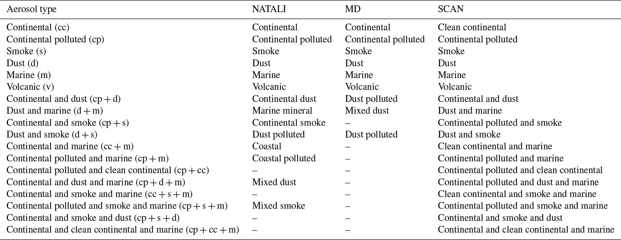
The maximum number of pure aerosol types that SCAN can assign to a layer is six, and the combination of them gives SCAN the capability to identify aerosols from different sources in a specific layer. In Table 1 one can find the pure aerosol types and the mixtures that SCAN has dealt with in this study. The whole classification procedure of SCAN is displayed in the flowchart in Fig. 2.
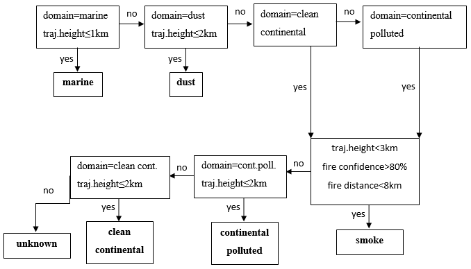
Figure 2Classification procedure of SCAN. This procedure is performed for each hour of the HYSPLIT back trajectory associated with each layer.
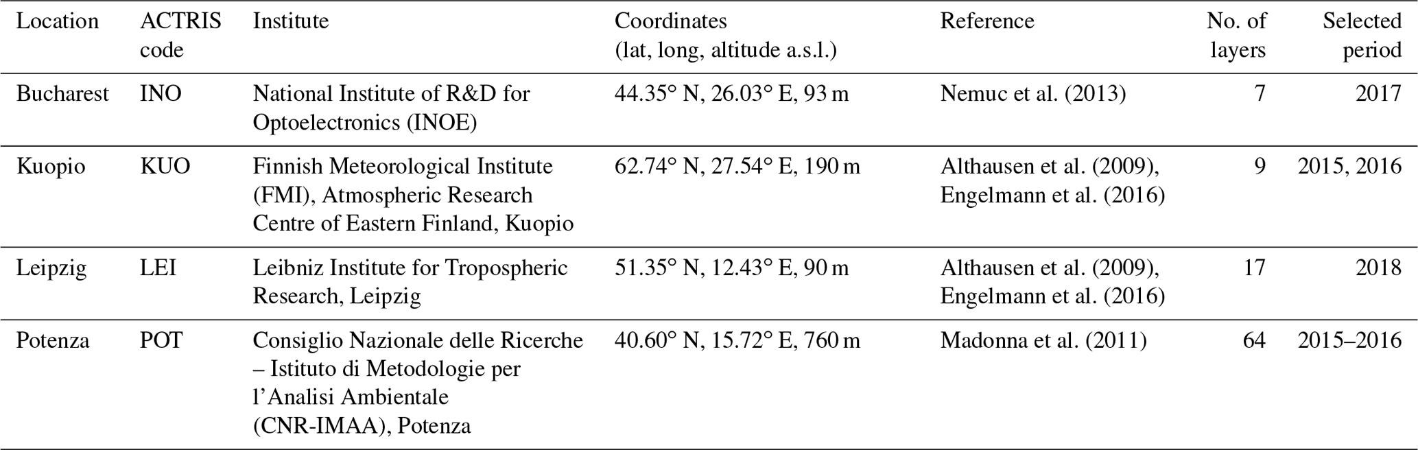
2.2 EARLINET lidar stations and data
The lidar station selection was based on the availability of the vertical profiles of a full set ( PLDR) of aerosol optical properties at several wavelengths: backscatter coefficient (b355, b532, b1064), extinction coefficient (e355, e532), lidar ratio (LR355, LR532), Ångström exponent (, , ), and particle linear depolarization ratio (PLDR532) at the EARLINET database during the period 2014–2018. Therefore, the selected lidar stations are the following: Bucharest, Romania; Kuopio, Finland; Leipzig, Germany; and Potenza, Italy (Table 2). Thus, 48 full sets ( PLDR) of aerosol optical properties of lidar observations from the aforementioned stations have been studied. For each data set and each aerosol layer, the geometrical layer boundaries (bottom, top) have been calculated according to Belegante et al. (2014). In total, 97 free tropospheric (FT) aerosol layers were obtained, and their mean aerosol optical properties (intensive and extensive) were calculated.
2.3 Case studies
In this section selected atmospheric layers involving different types of probed aerosols are presented. The performance of the three automated aerosol typing algorithms for aerosol classification is discussed in detail.
Figure 3 illustrates the vertical profiles of the aerosol optical properties, along with the mean values and standard deviations (inserted text) of the following: (3a) b355, b532, and b1064 (SR−1 Mm−1); (3b) e355 and e532 (Mm−1); (3c) LR355 and LR532 (SR); (3d) , , and ; and (3e) the PLDR532 (%) of the aerosol layer observed on 30 July 2015 over (i) Kuopio (19:25 UTC) and (ii) over Potenza (21:26 UTC). The bottom and top boundaries of the aerosol layer observed over Kuopio are estimated at 1.5 and 1.9 km a.s.l. (Fig. 3i, lower red and upper black horizontal line), respectively. For the same day, three different aerosol layers are detected over Potenza with corresponding values (Fig. 3ii) for the bottom (red horizontal line) and top (black horizontal line) of (1) 2.8 and 3.1 km a.s.l. (lower layer), (2) 3.4 and 3.9 km (middle layer), and (3) 4.5 and 5.4 km (upper layer), respectively.
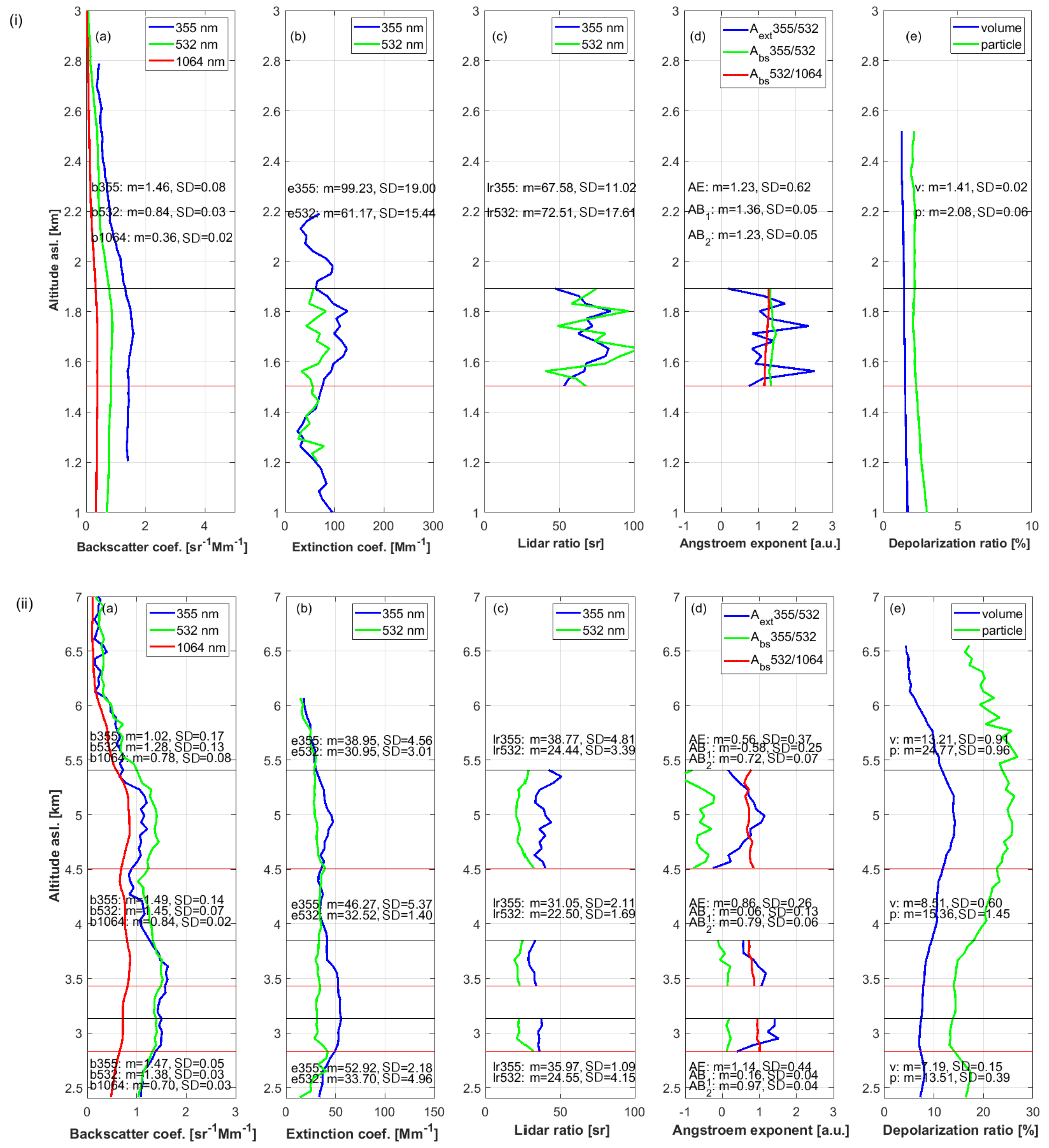
Figure 3Vertical profiles of the following aerosol optical properties observed over (i) Kuopio (19:25 UTC) and (ii) Potenza (21:26 UTC) on 30 July 2015, along with their mean values and standard deviations (inserted text): (a) b355, b532, b1064, (b) e355, e532, (c) LR355, LR532, (d) , , , (e) VDR532, and PLDR532.
The mean values of the intensive aerosol optical properties within the aerosol layer observed over Kuopio and Potenza on 30 July 2015 are also presented in Table 3. In particular, for the case of Kuopio, the LR355 values were found to be lower than those of LR532, the Ångström exponent (both extinction- and backscatter-related) was higher than 1.2, and PLDR532 had low values (<5 %), indicating fine absorbing aerosols. For the case of Potenza, the LR values were found to be low (<39 SR at 355 nm and <25 SR at 532 nm), while the Ångström exponents remained mainly below 1.0 for all three aerosol layers observed. The difference between these three aerosol layers is the value of PLDR532, which was found to ascend from 13.5 ± 0.4 % (bottom layer) to 15.4 ± 1.5 % (middle layer) and finally reached the value of 24.8 ± 1.0 % (top layer), indicating coarse semi-depolarizing aerosols at lower altitudes (<4.5 km) and highly depolarizing aerosols higher, probably of dust origin.
Table 3Mean values of the intensive optical properties of aerosol layers observed on 30 July 2015 over Kuopio and Potenza.
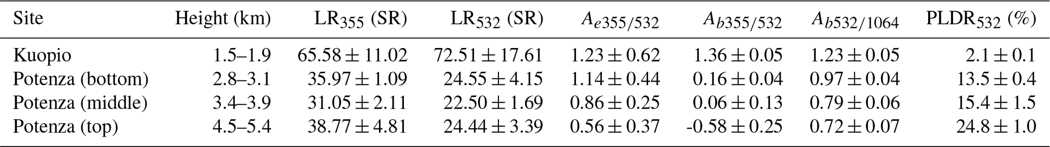
Figure 4 illustrates the 6 d (144 h) backward trajectory analysis for air masses ending on 30 July 2015 over the stations in (i) Kuopio (62.74∘ N, 27.54∘ E) at 1500 m a.s.l. (19:00 UTC) and (ii) Potenza (40.60∘ N, 15.72∘ E) at (1) 3000, (2) 3800, and (3) 5000 m a.s.l. (21:00 UTC). The color bar indicates the trajectory's height above sea level for each hour of its journey. According to Fig. 4i the air masses that reached Kuopio on that day at 1500 m a.s.l. (19:00 UTC) traveled from Ireland to southern Finland from 26 to 30 July at ∼ 1500 m a.s.l. and were probably affected by continental polluted and clean continental aerosol sources in northern Europe. The same air masses seem to also be affected by marine aerosols from 24 to 25 July when traveling at lower heights (<1000 m a.s.l.) over southern Ireland.
In contrast, the air masses that reached Potenza on 30 July 2015 at 3000 m a.s.l. (lower layer, Fig. 4ii) traveled at a height of ∼ 2000 m a.s.l. throughout their 6 d journey. These air masses started from northwestern Africa, remained in the area almost 3 d, and then passed over southern Spain before reaching Potenza. The aerosol layer observed over Potenza the same date and hour at 3800 m a.s.l. (middle layer, Fig. 3ii, a–b) originated over the northern Atlantic Ocean at a height of ∼ 5000 m a.s.l. 6 d before and slowly descended to lower altitudes before passing over northern Spain near ground level (Fig. 4ii, 2). In the following 2 d, the air mass traveled at a height of 2000–4000 m a.s.l. from Spain to Italy over the Mediterranean Sea before reaching Potenza.
Finally, the upper aerosol layer observed over Potenza at 5000 m a.s.l. (upper layer, Fig. 3ii, a–b) had a similar origin as the previous one except the first 3 d of its journey when the air masses traveled over the Atlantic Ocean at low altitudes (<1000 m a.s.l.), enhancing the marine contribution to that layer (Fig. 4ii, 3).
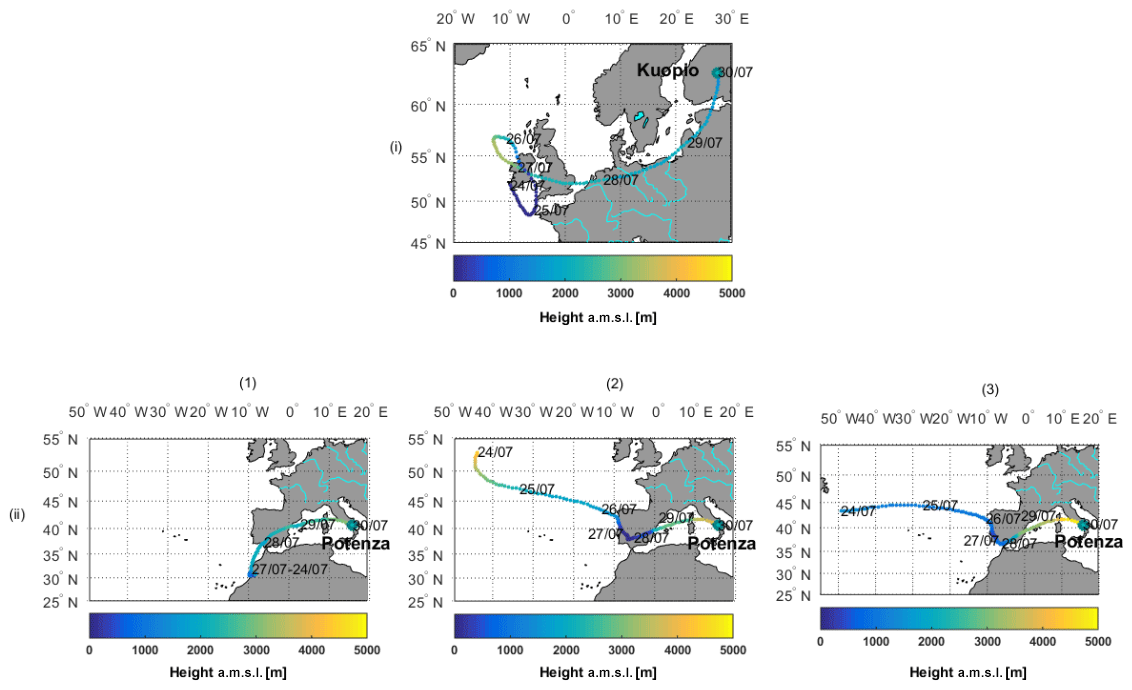
Figure 4HYSPLIT (GDAS Meteorological Data) 6 d (144 h) air-mass backward trajectory ending on 30 July 2015 over the lidar stations in (i) Kuopio (62.74∘ N, 27.54∘ E) at 1500 m. a.s.l. (19:00 UTC) and (ii) Potenza (40.60∘ N, 15.72∘ E) at (1) 3000, (2) 4000, and (3) 5000 m a.s.l. (21:00 UTC) using the model vertical velocity as a vertical motion calculation method. The color bar indicates the trajectory's height above mean sea level for each hour of its journey.
In Fig. 5 we present the classification of the aerosol layers under study by (a) NATALI, (b) MD, and (c) SCAN. The aerosol type results are given concerning the classification by NATALI. Concerning the MD classification, the normalized probabilities of each aerosol type assumed by MD are also given. Finally, concerning the classification of the aerosols by SCAN, the time (in hours) within which the air mass circulated over specified domains is also provided. It should be noted here that different colors refer to different aerosol types or aerosol mixtures.
Thus, in Fig. 5 we observe that NATALI classified the aerosol layer observed over Kuopio as continental polluted. MD also gave the highest probability (65 %) for the same layer to be of continental polluted origin and typed it as such, while the second-closest probability was 11 % smoke. Finally, SCAN attributed 24 h to that air mass and classified it as continental polluted. Moreover, 17 h were attributed as clean continental and 2 h as marine out of the 144 h of the air-mass backward trajectory, so it was finally classified as a cp + cc + m mixture (Fig. 5ia–c). For the remaining 101 h of the air-mass backward trajectory that SCAN did not take into account, it was assumed that the air mass traveled without being affected by any aerosol source as a result of the combination of the height and domain limitations, criteria that SCAN take into account during its classification process. Taking into account these criteria and the air-mass back trajectory provided by HYSPLIT, we would expect that SCAN should have counted more hours for the air mass attributed as marine. This is because of the predefined domains on the map as possible aerosol sources, which reduces the spatial accuracy of the classification method (Fig. 1). Therefore, we can see that the final results of the three methods (Fig. 5ia–c) are in good agreement concerning the layer observed over Kuopio, although MD and SCAN can provide additional information on the constituents of the aerosol layer.
On the other hand, the classification results for the aerosol layers observed over Potenza on t30 July 2015 are more complex (Fig. 3ii). NATALI classified the lower and middle aerosol layers as marine/cc and the upper one as mineral mixtures/volcanic. However, regarding the lower and middle aerosol layers, they are highly unlikely to be of marine origin, as they are not affected by the sea spray at these heights (>2.5 km a.s.l.). These erroneous classification results must have been affected by the low LR values (22–35 ± 5 SR).
In this case MD gave the aforementioned lower aerosol layer a 41 % probability to be of continental polluted origin, while there was also a 22 % probability for the layer to be clean continental. MD also classified the middle aerosol layer as marine with a 63 % probability, while it seems to attribute a 16 % probability to the continental polluted aerosol type. Again, the classification results for the lower and middle layers have probably been affected by the low LR values. Concerning the upper aerosol layer observed over Potenza, MD failed to characterize it, as it gave nearly equal probabilities to its possible aerosol types.
Taking into account the results provided by SCAN concerning the lower aerosol layer observed above Potenza, SCAN counted 78 h as dust and 11 h as continental polluted, finally classifying the aerosols as a mixture of continental polluted + dust. Concerning the middle aerosol layer, SCAN counted 64 h as continental polluted aerosols (out of 144 total hours), while one would expect a contribution of dust aerosols as well, according to both PLDR532 values and the origin of the air masses based on the air-mass backward-trajectory analysis. This indicates, again, that the predefined domains on the map of possible aerosol sources reduce the spatial accuracy of the classification method, especially when it comes to the southern Mediterranean Sea in the vicinity of Sahara. In these cases, an atmospheric dust model (e.g., BSC DREAM) should be used synergistically. Finally, concerning the upper aerosol layer observed above Potenza, SCAN counted 66 h as continental polluted aerosols and 44 h as marine aerosols, the latter again being highly improbable at that height (∼ 5 km a.s.l.), as previously explained. Again, it becomes obvious that an atmospheric dust model should be used synergistically with the SCAN results when we deal with air-mass backward trajectories passing over the southern Mediterranean Sea due to the vicinity of Sahara.
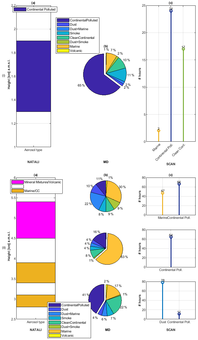
Figure 5Aerosol layers observed over (i) Kuopio and (ii) Potenza at 3 (bottom), 3.8 (middle), and 5 km a.s.l. (top) on 30 July 2015 classified by (a) NATALI, (b) MD, and (c) SCAN.
So far, 97 FT aerosol layers have been classified by the three aforementioned classification algorithms. The results have been separated into aerosol layers according to aerosol types as follows: the 1 type (Fig. 6, blue) and mixture (Fig. 6, cyan) categories represent the aerosol layers that consist of one and two or more aerosol types, respectively. The other category consists of cases that NATALI marked as aerosol type/cloud-contaminated (i.e., marine/cc), and finally, the unknown category (Fig. 6, yellow) consists of the cases for which the method was unable to identify the source of the observed aerosol layers. All the aerosol types and mixtures considered by each algorithm are demonstrated in Table 1.
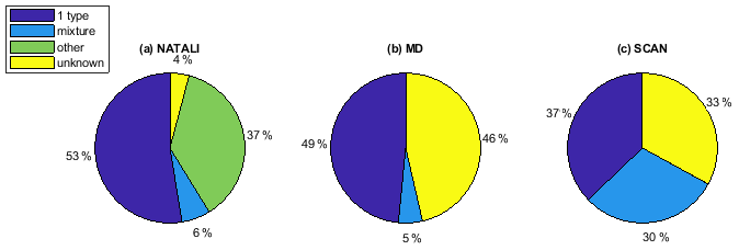
Figure 6Percentages of classified aerosol layers by (a) NATALI, (b) MD, (c) SCAN. Blue: 1 type aerosol layers, cyan: mixtures, green: other types, yellow: unknown constitution of aerosol layers.
It can be concluded that NATALI (Fig. 6a) is able to classify the highest number of cases (94 cases), while MD (Fig. 6b) failed to classify a high number of cases (46 %) with a lower percentage of aerosols classified as “mixture” types (5 %), which is a reasonable outcome given that the MD scheme considers only two aerosol mixtures, while NATALI and SCAN have many more. Finally, the SCAN algorithm (Fig. 6c) classified 37 % of the aerosol layers (36 layers) as 1 type, 30 % (29 layers) as aerosol mixtures, and 32 % (32 layers) as unknown types.
3.1 Comparison of aerosol classification codes
In Fig. 7 we present a comparison of the classification results obtained using the pairs of (a) NATALI and MD, (b) MD and SCAN, and (c) SCAN and NATALI. The number of aerosol layers classified as indicated by the row i and the column j is given inside each (i,j) square. For example, the number of aerosol layers classified as being 1 type by MD but as a mixture of aerosols by SCAN is shown inside the (1 type – mixture) square (there are 16 such cases for this example in Fig. 7b).
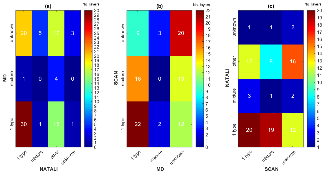
Figure 7Comparison between classified aerosol layers by (a) NATALI and MD, (b) MD and SCAN, and (c) SCAN and NATALI. The number of classified aerosol layers as indicated by the i row and the j column is given inside each (i,j) square.
In Fig. 7a it can be seen that the 45 cases classified as unknown by MD were classified as 1 type (20 cases), a mixture (5 cases), or other (17 cases) by NATALI and 1 type (12 cases) or a mixture (13 cases) by SCAN (Fig. 7b). Furthermore, it seems that MD is unable to discriminate the different aerosol types inside the other layers according to NATALI (Fig. 7a) and the mixture layers according to SCAN, labeling them as 1 type (Fig. 7b), which is probably because only two aerosol mixtures are considered by MD. Concerning the 29 unknown cases classified by SCAN, 20 of them were also identified as unknown by MD (Fig. 7b), and they were almost equally separated into 1 type (12 cases) and other (16 cases) by NATALI (Fig. 7c).
3.1.1 NATALI versus MD
Figure 8a presents a comparison between the cases that MD classified as 1 type or a mixture against those classified as other by NATALI, while Fig. 8b shows the number of aerosol layers that MD classified as unknown and NATALI as 1 type. Finally, in Fig. 8c we present the number of aerosol layers that MD classified as unknown and NATALI as a mixture or other. The pie charts above each bar (Fig. 8b) and each stem (Fig. 8c) reveal the mean frequencies of each aerosol type as calculated by MD.
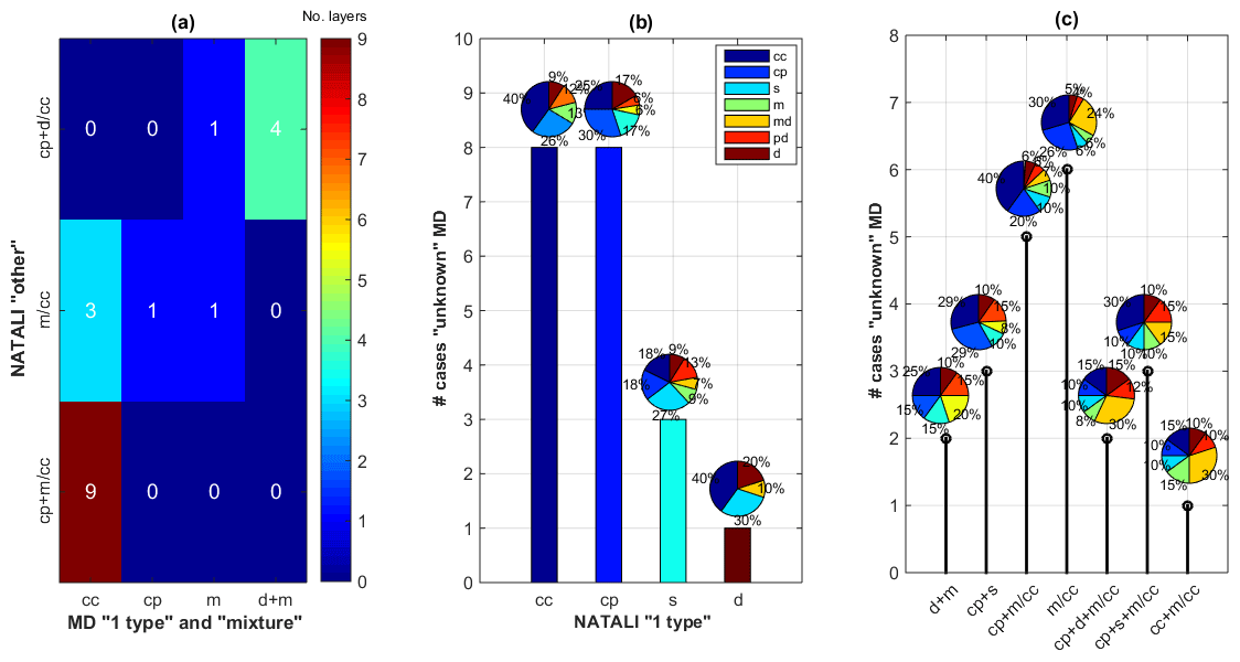
Figure 8(a) Comparison between the cases classified by MD as 1 type or mixture and as other by NATALI. (b) Number of aerosol layers classified by MD as unknown and as 1 type by NATALI. (c) Number of aerosol layers classified by MD as unknown and as mixture or other by NATALI. The pie charts above each bar and each stem reveal the mean frequencies of each aerosol type as calculated by MD.
The inability of MD to classify the aerosol layers according to NATALI's classification (Fig. 8a) can be attributed to the characteristics of the aerosol layers not being well-modeled by the algorithm, which means that the intensive parameters are not within the accepted “borders” of the predefined classes of the algorithm. Concerning the 1 type aerosol layers according to NATALI (Fig. 8b), MD would have predicted them correctly if the labeling of these layers by MD was achieved by considering a higher percentage of aerosol types, as the pie charts above each bar indicate (Fig. 8b). This does not seem to be the case for the dust type labeled by NATALI, to which MD gave a 40 % probability to be continental polluted, 30 % smoke, and only 30 % dust and mixed dust (Fig. 8b). Concerning the mixture and other according to NATALI (Fig. 8c), it seems that MD found a high contribution of dust and mixtures of dust aerosols (approximately 50 %) inside these layers (yellow, orange, and dark red aerosol types according to the pie charts above the stems).
3.1.2 MD versus SCAN
Figure 9a presents a comparison between the cases that were classified by MD as 1 type and as a mixture by SCAN, while Fig. 9b shows the number of aerosol layers classified by MD as unknown and as 1 type by SCAN. Finally, Fig. 9c presents the number of aerosol layers classified by MD as unknown and as a mixture or other by SCAN. The pie charts above each bar (Fig. 9b) and each stem (Fig. 9c) reveal the mean frequencies of each aerosol type as calculated by MD.
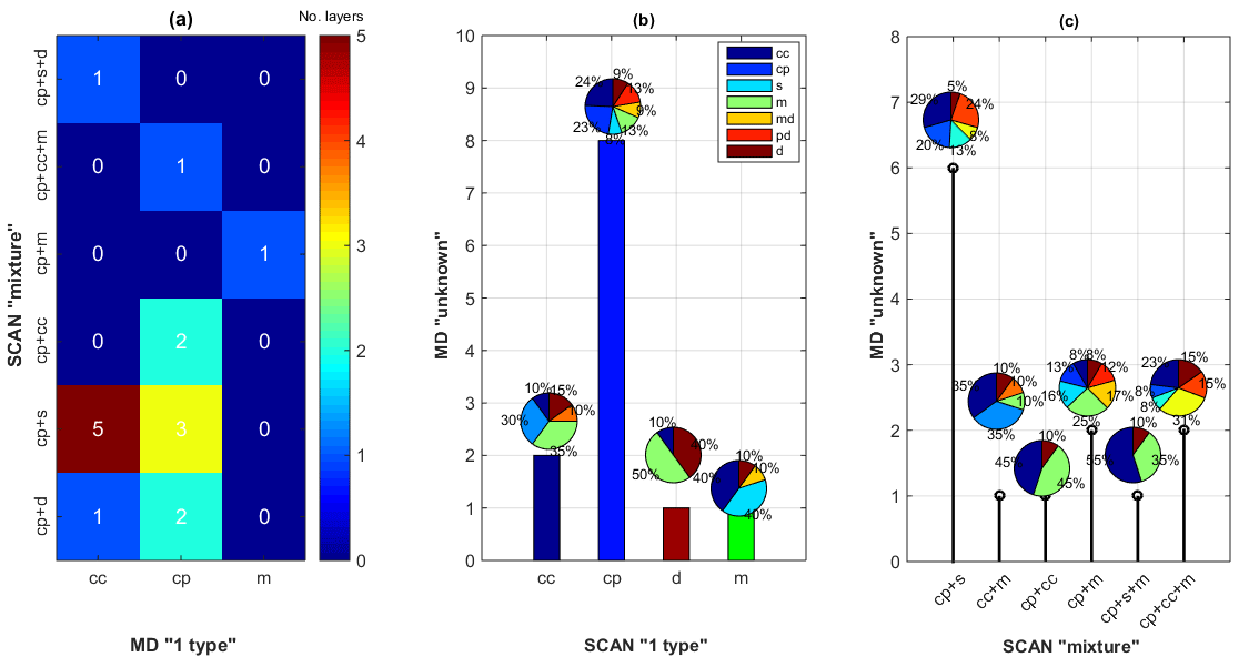
Figure 9(a) Comparison between the cases that were classified by MD as 1 type and as mixture by SCAN. (b) Number of aerosol layers classified by MD as unknown and as 1 type by SCAN. (c) The number of aerosol layers classified by MD as unknown and as mixture or other by SCAN. The pie charts above each bar and each stem reveal the mean frequencies of each aerosol type as calculated by MD.
The misclassification of an aerosol layer by MD compared to the classification as a continental polluted and smoke layer by SCAN (Fig. 9a) could again be attributed to the location of the observation compared to the location of the predefined aerosol types for the MD classification algorithm, which depend on the aerosol optical properties of the studied layers. Additionally, it seems that the aerosol optical properties of the mixture of continental polluted and smoke by SCAN are attributed to either clean continental or continental polluted aerosols by MD (Fig. 9a). From the cases that MD classified as unknown, eight are classified as continental polluted (cp) by SCAN (Fig. 9b), while another six cases are classified as continental polluted and smoke (cp + s) (Fig. 9c). Finally, from these unknown cases by MD, there are another 11 cases that SCAN classified as clean continental (two cases), dust (one case), marine (one case; Fig. 9b), clean continental and marine (one case), continental polluted and clean continental (one case), continental polluted and marine (two cases), continental polluted, smoke, and marine (one case), or continental polluted, clean continental, and marine (two cases; Fig. 9c).
3.1.3 SCAN versus NATALI
Figure 10 presents a comparison between the cases that (a) SCAN classified as a mixture and NATALI as 1 type, (b) SCAN classified as 1 type and NATALI as other, and (c) SCAN classified as a mixture and NATALI as other.
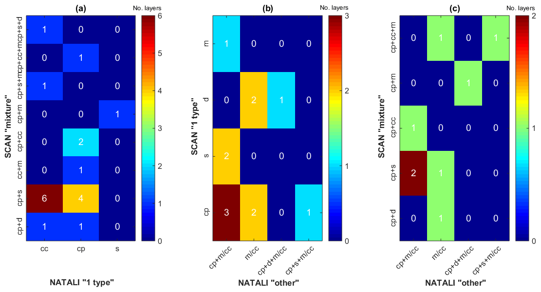
Figure 10Comparison between the cases classified by (a) SCAN as mixture and as 1 type by NATALI, (b) SCAN as 1 type and as other by NATALI, and (c) SCAN as mixture and as other by NATALI.
From Fig. 10 it can be concluded that of the 12 cases that SCAN classified as continental polluted and smoke (cp + s), NATALI classified 6 of them as clean continental (cc), 4 as continental polluted (cp) (Fig. 10a), and 2 as continental polluted and marine/cloud-contaminated (cp + m/cc) (Fig. 10c). Moreover, of the six cases that SCAN classified as continental polluted (cp), three of them were classified as continental polluted and marine or cloud-contaminated (cp + m/cc), two as marine/cloud-contaminated (m/cc), and only one as continental polluted, smoke, and marine or cloud-contaminated (cp + s + m/cc) by NATALI (Fig. 10b). It seems that the aerosol optical properties of this mixture are attributed to either the clean continental or continental polluted aerosol types based on the NATALI classification.
3.2 Aerosol optical properties
The mean values of the aerosol optical properties derived from the NATALI, MD, and SCAN classification for each aerosol type are presented in Table 4 and discussed in this section. The correspondence between the aerosol types and the terminology defined by the classification methods is presented in Table 1.
3.2.1 Clean continental (cc) aerosols
Aerosol layers classified as clean continental by both NATALI and MD present medium LR355 values (45–46 ± 5 SR), medium to low LR532 values (37–39 ± 5 SR), medium and values (1.0 ± 0.3), high values (2.0 ± 0.3), and low PLDR values at 532 nm (3 ± 1 %). These values are in accordance with others reported in previous studies concerning cc aerosols (Ansmann et al., 2001; Omar et al., 2009; Giannakaki et al., 2010).
Table 4Mean values and standard deviations of aerosol optical properties according to each classification method.

3.2.2 Continental polluted (cp) aerosols
Aerosol layers classified as continental polluted by both NATALI and MD present medium LR355 nm (57 ± 6 SR), slightly higher LR532 values (62 ± 7 SR), medium , , and values (1.1–1.4 ± 0.3), and low PLDR values at 532 nm (3 ± 1 %). On the other hand, the aerosol layers similarly classified by SCAN present medium LR355 values (50 ± 6 SR) and LR532 values (49 ± 5 SR), medium , and values (1.0–1.5 ± 0.3), and low PLDR values at 532 nm (3 ± 1 %). These values are also in accordance with those reported in previous studies concerning this type of aerosol (Müller et al., 2007; Giannakaki et al., 2010; Gross et al., 2013; Burton et al., 2013; Mattis et al., 2008). The similarity of these values to those of the clean continental aerosol type is the reason why it remains difficult to distinguish between these two aerosol types.
3.2.3 Smoke (s) aerosols
Smoke aerosol layers according to SCAN show medium LR355 values (50 ± 5 SR), medium to small LR532 values (37 ± 4 SR), medium and values (0.9–1.3 ± 0.3), medium to high values (1.6 ± 0.3), and low PLDR values at 532 nm (3 ± 1 %). These values are in accordance with those reported in previous studies concerning this type of aerosol (Wandinger et al., 2002; Müller et al., 2005, 2007; Burton et al., 2013; Baars et al., 2012; Balis, et al., 2003; Papanikolaou, et al., 2020). Again, the similarity of these values to those of the clean continental and continental polluted aerosol types is the reason why it remains difficult to distinguish between these three aerosol types.
3.2.4 Marine/cloud-contaminated (m/cc) aerosols
Aerosol layers classified as marine/cloud-contaminated by NATALI showed low values of LR355 (35 ± 4 SR), even lower LR532 values (27 ± 3 SR), small to medium and values (0.9-1.0 ± 0.3), increased values (1.7 ± 0.3), and low PLDR532 values (4 ± 2 %). These values are in accordance with those reported by Cattrall et al. (2005), Burton et al. (2012, 2013), and Dawson, et al. (2015) concerning marine aerosols.
3.2.5 Dust and marine aerosols (d&m)
Concerning the dust and marine mixture according to the MD algorithm classification, these aerosols showed medium LR355 values (43 ± 4 SR), low LR532 values (46 ± 5 SR), small , (0.0–0.7 ± 0.2), values (−0.2 ± 0.2), and medium PLDR532 values (15 ± 5 %). These values indicate large and depolarizing aerosol particles, confirming the type of these particles as a mixture of dust and marine ones, according to Burton et al. (2012) and Papagiannopoulos et al. (2016).
3.2.6 Continental polluted and smoke (cp&s) aerosols
The continental polluted and smoke mixed aerosols classified according to SCAN showed medium LR355 values (52 ± 8 SR), medium LR532 values (47 ± 7 SR), medium and values (0.8–1.3 ± 0.4), high values of (1.5 ± 0.4), and low values of PLDR532 (4 ± 2 %). The medium LR355 and LR532 values indicate continental polluted aerosols (Müller et al., 2007; Giannakaki et al., 2010; Gross et al., 2013; Burton et al., 2013; Papanikolaou, et al., 2020), while the high values indicate smoke aerosols (Wandinger et al., 2002; Müller et al., 2005).
3.2.7 Continental polluted and marine (cp&m) aerosols
The continental polluted and marine mixture according to NATALI showed a large difference between the LR355 and LR532 values, with the latter being smaller (LR355=69 ± 11, LR532=31 ± 5.3 SR). The , , and PLDR at 532 nm showed low values (0.9 ± 0.4, −1.2 ± 0.4, 2.7 ± 1.6, respectively), while the showed large values (1.3 ± 0.2). SCAN showed medium LR355 values (45 ± 6 SR), increased LR532 values (55 ± 7 SR), low , , and values (0.3–0.7 ± 0.3), and low PLDR532 values (8 ± 4 %). The low PLDR values are indicative of non-depolarizing aerosols such as continental polluted (Müller et al., 2007; Giannakaki et al., 2010; Gross et al., 2013; Burton et al., 2013) and marine aerosols (Gross et al., 2011; Burton et al., 2012, 2013; Gross et al., 2013). Additionally, the low , , and values are indicative of coarse-mode aerosols such as marine, while the increased LR532 values are more indicative of continental polluted aerosols rather than marine ones.
3.2.8 Continental polluted, dust, and marine or clean continental (cp&d&m/cc) aerosols
Finally, the continental polluted, dust, and marine or cloud-contaminated aerosol mixture classified by NATALI showed medium LR355 values (41 ± 4 SR), medium LR532 values (43 ± 5 SR), low , , and values (−0.1–0.7 ± 0.3), and medium PLDR532 values (13 ± 4 %). Here, the medium PLDR values are indicative of dust mixtures (Gross et al., 2011, 2016; Burton et al., 2013), while the low , , and values are indicative of coarse-mode aerosols, such as dust and marine.
In this study, we compared three independent aerosol classification methods: a neural network aerosol typing algorithm, the Mahalanobis distance automatic aerosol type classification, and a source classification analysis using 97 free tropospheric aerosol layers from four EARLINET stations (Bucharest, Kuopio, Leipzig, and Potenza) from 2014–2018. NATALI is an automated aerosol layer classification neural network depending on the aerosol optical properties () directly obtained from the EARLINET database. MD is an automated aerosol layer classification algorithm depending on the mean values of the aerosol optical properties (, LR532, LR532 LRλ355, PLDR532, and ) of the probed atmospheric layers. SCAN, introduced for the first time in this study, is based on the automatization of the typical classification method, while its classification procedure is based on the amount of time that an air parcel spends over specific pre-characterized aerosol source regions and a number of additional criteria, as analytically presented.
We concluded that NATALI showed a lower percentage (4 %) of unclassified layers. When compared to MD, NATALI's X or cloud-contaminated aerosol layers (where X is either an aerosol type or a mixture) are classified by MD as clean continental layers, except when X is a mixture of dust aerosols. When compared, SCAN's continental polluted and smoke layers are classified by NATALI as either clean continental or continental polluted.
Furthermore, we found that MD was unable to classify almost 50 % of the layers under study. Compared to NATALI, these layers either belong to one single aerosol type or to aerosol mixtures. Concerning MD's unknown category and NATALI's one single aerosol type, we showed that MD's mean percentages predict the aerosol type of each layer quite well, even though this aerosol type is not chosen by the classification process of MD. Concerning MD's unknown and NATALI's mixture categories, the MD algorithm revealed an increased contribution of dust aerosols (approximately 50 %) inside the studied aerosol layers. Compared to SCAN, MD's unknown layers are mainly either continental polluted or continental polluted and smoke. Finally, SCAN's continental polluted and smoke layers are classified by MD as either clean continental or continental polluted.
We found that the SCAN code successfully managed to classify more than 50 % of the layers studied either as a single aerosol type or as mixtures of different aerosols. Being independent of aerosol optical properties, SCAN provides the advantage that its classification process is not affected by overlapping values of the optical properties representing more than one aerosol type (clean continental, continental polluted, smoke). Furthermore, it has no limitations concerning its ability to classify aerosol mixtures, an advantage that arises from the air-mass trajectory analysis and the relevant aerosol sources on the ground. Finally, it can be useful for all types of lidar systems (independently of the number of channels used) and for other network-based systems (radar profilers, sun photometers).
The aerosol lidar profiles used in this study are available upon registration from the EARLINET web page at https://data.earlinet.org/earlinet/login.zul (Pappalardo et al., 2014).
DN, NP, and EG distributed the NATALI, MD, and SCAN algorithms, respectively. CAP created algorithms that produced the maps presented in this work. EG had the idea for this paper. MM upgraded the SCAN algorithm, collected the lidar data, made the comparison, analyzed the results, and wrote the paper. All authors participated in scientific discussions on this study and reviewed and edited the paper during its preparation process.
The authors declare that they have no conflict of interest.
This article is part of the special issue “EARLINET aerosol profiling: contributions to atmospheric and climate research”. It is not associated with a conference.
The authors acknowledge support through ACTRIS under grant agreement no. 262254 from the European Commission Seventh Framework Programme (FP7/2007–2013) and ACTRIS-2 under grant agreement no. 654109 from the Horizon 2020 research and innovation program of the European Commission. The authors acknowledge EARLINET for providing aerosol lidar profiles available at https://data.earlinet.org/ (last access: 1 August 2020). The authors gratefully acknowledge the NOAA Air Resources Laboratory (ARL) for the provision of the HYSPLIT transport and dispersion model as well as the READY website (http://www.ready.noaa.gov, last access: 1 August 2020) used in this publication. We acknowledge the use of data products and imagery from the Land, Atmosphere Near-real-time Capability for EOS (LANCE) system operated by NASA's Earth Science Data and Information System (ESDIS) with funding provided by NASA headquarters.
This research has been supported by the Hellenic Foundation for Research and Innovation (grant no. 669) and the PANhellenic infrastructure for Atmospheric Composition and climatE change (grant no. MIS 5021516), which is implemented under the action “Reinforcement of the Research and Innovation Infrastructure” funded by the operational program “Competitiveness, Entrepreneurship and Innovation” (NSRF 2014–2020), and co-financed by Greece and the European Union (European Regional Development Fund).
This paper was edited by Eduardo Landulfo and reviewed by three anonymous referees.
Althausen, D., Engelmann, R., Baars, H., Heese, B., Ansmann, A., Müller, D., and Komppula, M.: Portable raman lidar pollyxt for automated profiling of aerosol backscatter, extinction, and depolarization, J. Atmos. Ocean. Technol., 26, 2366–2378, https://doi.org/10.1175/2009JTECHA1304.1, 2009.
Amiridis, V., Giannakaki, E., Balis, D. S., Gerasopoulos, E., Pytharoulis, I., Zanis, P., Kazadzis, S., Melas, D., and Zerefos, C.: Smoke injection heights from agricultural burning in Eastern Europe as seen by CALIPSO, Atmos. Chem. Phys., 10, 11567–11576, https://doi.org/10.5194/acp-10-11567-2010, 2010.
Ansmann, A., Wagner, F., Althausen, D., Müller, D., Herber, A., and Wandinger, U.: European pollution outbreaks during ACE 2: Lofted aerosol plumes observed with Raman lidar at the Portuguese coast, J. Geophys. Res. Atmos., 106, 20725–20733, https://doi.org/10.1029/2000JD000091, 2001.
Baars, H., Ansmann, A., Althausen, D., Engelmann, R., Heese, B., Mller, D., Artaxo, P., Paixao, M., Pauliquevis, T., and Souza, R.: Aerosol profiling with lidar in the Amazon Basin during the wet and dry season, J. Geophys. Res. Atmos., 117, 1–16, https://doi.org/10.1029/2012JD018338, 2012.
Balis, D. S., Amiridis, V., Zerefos, C., Gerasopoulos, E., Andreae, M., Zanis, P., Kazantzidis, A., Kazadzis, S., and Papayannis, A.: Raman lidar and sunphotometric measurements of aerosol optical properties over Thessaloniki, Greece during a biomass burning episode, Atmos. Environ., 37, 4529–4538, https://doi.org/10.1016/S1352-2310(03)00581-8, 2003.
Basart, S., Pérez, C., Nickovic, S., Cuevas, E., and Baldasano, J.: Development and evaluation of the BSC-DREAM8b dust regional model over Northern Africa, the Mediterranean and the Middle East, Tellus B, 64, 18539, https://doi.org/10.3402/tellusb.v64i0.18539, 2012.
Belegante, L., Nicolae, D., Nemuc, A., Talianu, C., and Derognat, C.: Retrieval of the boundary layer height from active and passive remote sensors. Comparison with a NWP model, Acta Geophys., 62, 276–289, https://doi.org/10.2478/s11600-013-0167-4, 2014.
Boucher, O., Randall, D., Artaxo, P., Bretherton, C., Feingold, G., Forster, P., Kerminen, V.-M., Kondo, Y., Liao, H., Lohmann, U., Rasch, P., Satheesh, S. K., Sherwood, S., Stevens, B., and Zhang, X. Y.: Clouds and Aerosols, in: Climate Change 2013: The Physical Science Basis. Contribution of Working Group I to the Fifth Assessment Report of the Intergovernmental Panel on Climate Change, edited by: Stocker, T. F., Qin, D., Plattner, G.-K., Tignor, M., Allen, S. K., Boschung, J., Nauels, A., Xia, Y., Bex, V., and Midgley, P. M., Cambridge University Press, Cambridge, United Kingdom and New York, NY, USA, 2013.
Burton, S. P., Ferrare, R. A., Hostetler, C. A., Hair, J. W., Rogers, R. R., Obland, M. D., Butler, C. F., Cook, A. L., Harper, D. B., and Froyd, K. D.: Aerosol classification using airborne High Spectral Resolution Lidar measurements-methodology and examples, Atmos. Meas. Tech., 5, 73–98, https://doi.org/10.5194/amt-5-73-2012, 2012.
Burton, S. P., Ferrare, R. A., Vaughan, M. A., Omar, A. H., Rogers, R. R., Hostetler, C. A., and Hair, J. W.: Aerosol classification from airborne HSRL and comparisons with the CALIPSO vertical feature mask, Atmos. Meas. Tech., 6, 1397–1412, https://doi.org/10.5194/amt-6-1397-2013, 2013.
Cattrall, C., Reagan J., Thome K., and Dubovik O.: Variability of aerosol and spectral lidar and backscatter andextinction ratios of key aerosol types derived from selected Aerosol Robotic Network locations, J. Geophys. Res., 11, D10S11, https://doi.org/10.1029/2004JD005124, 2005.
Davies, D. K., Ilavajhala, S., Wong, M. M., and Justice, C. O.: Fire information for resource management system: Archiving and distributing MODIS active fire data, IEEE T. Geosci. Remote Sens., 47, 72–79, https://doi.org/10.1109/TGRS.2008.2002076, 2009.
Dawson, K. W., Meskhidze, N., Josset, D., and Gassó, S.: Spaceborne observations of the lidar ratio of marine aerosols, Atmos. Chem. Phys., 15, 3241–3255, https://doi.org/10.5194/acp-15-3241-2015, 2015.
Draxler, R. R. and Hess, G. D.: An overview of HYSPLIT_4 modelling system for trajectories, dispersion and deposition, Aust. Met. Mag., 47, 295–308, 2013.
Freudenthaler, V., Esselborn, M., Wiegner, M., Heese, B., Tesche, M., Ansmann, A., Müller, D., Althausen, D., Wirth, M., Fix, A., Ehret, G., Knippertz, P., Toledano, C., Gasteiger, J., Garhammer, M., and Seefeldner, M.: Depolarization ratio profiling at several wavelengths in pure Saharan dust during SAMUM 2006, Tellus B, 61, 165–179, https://doi.org/10.1111/j.1600-0889.2008.00396.x, 2009.
Georgoulias, A. K., van der A, R. J., Stammes, P., Boersma, K. F., and Eskes, H. J.: Trends and trend reversal detection in 2 decades of tropospheric NO2 satellite observations, Atmos. Chem. Phys. 19, 6269–6294, https://doi.org/10.5194/acp-19-6269-2019, 2019.
Giannakaki, E., Balis, D. S., Amiridis, V., and Zerefos, C.: Optical properties of different aerosol types: Seven years of combined Raman-elastic backscatter lidar measurements in Thessaloniki, Greece, Atmos. Meas. Tech., 3, 569–578, https://doi.org/10.5194/amt-3-569-2010, 2010.
Giannakaki, E., Van Zyl, P. G., Müller, D., Balis, D., and Komppula, M.: Optical and microphysical characterization of aerosol layers over South Africa by means of multi-wavelength depolarization and Raman lidar measurements, Atmos. Chem. Phys., 16, 8109–8123, https://doi.org/10.5194/acp-16-8109-2016, 2016.
Giglio, L., Descloitres, J., Justice, C. O., and Kaufman, Y. J.: An enhanced contextual fire detection algorithm for MODIS, Remote Sens. Environ., 87, 273–282, https://doi.org/10.1016/S0034-4257(03)00184-6, 2003.
Gross, S., Esselborn, M., Weinzierl, B., Wirth, M., Fix, A., and Petzold, A.: Aerosol classification by airborne high spectral resolution lidar observations, Atmos. Chem. Phys., 13, 2487–2505, https://doi.org/10.5194/acp-13-2487-2013, 2013.
Hamill, P., Piedra, P., and Giordano, M.: Simulated polarization as a signature of aerosol type, Atmos. Environ., 224, 117348, https://doi.org/10.1016/j.atmosenv.2020.117348, 2020.
Ho, S. P., Peng, L., Anthes, R. A., Kuo, Y. H., and Lin, H. C.: Marine boundary layer heights and their longitudinal, diurnal, and interseasonal variability in the southeastern Pacific using COSMIC, CALIOP, and radiosonde data, J. Clim., 28, 2856–2872, https://doi.org/10.1175/JCLI-D-14-00238.1, 2015.
Hobbs, P. V.: Aerosol-cloud interactions, in: Aerosol-Cloud-Climate Interactions, Academic, San Diego, California, 1993.
Justice, C. O., Giglio, L., Korontzi, S., Owens, J., Morisette, J. T., Roy, D., Descloitres, J., Alleaume, S., Petitcolin, F., and Kaufman, Y.: The MODIS fire products, Remote Sens. Environ., 83, 244–262, https://doi.org/10.1016/S0034-4257(02)00076-7, 2002.
Kaufman, Y. J., Justice, C. O., Flynn, L .P., Kendall, J. D., Prins, E. M., Giglio, L., Ward, D. E., Menzel, W. P., and Setzer, A. W.: Potential global fire monitoring from EOS-MODIS, J. Geophys. Res., 103, 32215–32238, 1998.
Koepke, P., Hess, M., Schult, I., and Shettle, E. P.: Global Aerosol Data Set, Report No. 243, MPI Hamburg, Germany, 44 pp., 1997.
Madonna, F., Amodeo, A., Boselli, A., Cornacchia, C., Cuomo, V., D'Amico, G., Giunta, A., Mona, L., and Pappalardo, G.: CIAO: The CNR-IMAA advanced observatory for atmospheric research, Atmos. Meas. Tech., 4, 1191–1208, https://doi.org/10.5194/amt-4-1191-2011, 2011.
Mattis, I., Siefert, P., Müller, D., Tesche, M., Hiebsch, A., Kanitz, T., Schmidt, J., Finger, F., Wandinger, U., and Ansmann, A.: Volcanic aerosol layers observed with multiwavelength Raman lidar over central Europe in 2008–2009, J. Geophys. Res.-Atmos., 115, 1–9, https://doi.org/10.1029/2009JD013472, 2010.
Mishchenko, M. I., Travis, L. D., and Mackowski, D. W.: T-matrix computations of light scattering by nonspherical particles: A review, J. Quant. Spectrosc. Radiat. Transf., 55, 535–575, https://doi.org/10.1016/0022-4073(96)00002-7, 1996.
Müller, D., Mattis, I., Wandinger, U., Ansmann, A., Althausen, D., and Stohl, A.: Raman lidar observations of aged Siberian and Canadian forest-fire smoke in the free troposphere over Germany in 2003: Microphysical particle characterization, J. Geophys. Res., 110, D17201, https://doi.org/10.1029/2004JD005756, 2005.
Müller, D., Ansmann, A., Mattis, I., Tesche, M., Wandinger, U., Althausen, D., and Pisani, G.: Aerosol-type-dependent lidar ratios observed with Raman lidar, J. Geophys. Res.-Atmos., 112, 1–11, https://doi.org/10.1029/2006JD008292, 2007.
Nemuc, A., Vasilescu, J., Talianu, C., Belegante, L., and Nicolae, D.: Assessment of aerosol's mass concentrations from measured linear particle depolarization ratio (vertically resolved) and simulations, Atmos. Meas. Tech., 6, 3243–3255, https://doi.org/10.5194/amt-6-3243-2013, 2013.
Nicolae, D., Talianu, C., Ionescu, C., Ciobanu, M., and Ciuciu, J.: Aerosol statistics and pollution forecast based on lidar measurements in Bucharest, Romania, Lidar Technol. Tech. Meas. Atmos. Remote Sens., 59840, https://doi.org/10.1117/12.627727, 2005.
Nicolae, D., Talianu, C., Ciuciu, J., Ciobanu, M., and Babin, V.: LIDAR monitoring of aerosols loading over Bucharest, J. Optoelectron. Adv. Mater., 8, 238–242, 2006.
Nicolae, D., Nemuc, A., Müller, D., Talianu, C., Vasilescu, J., Belegante, L., and Kolgotin, A.: Characterization of fresh and aged biomass burning events using multiwavelength Raman lidar and mass spectrometry, J. Geophys. Res.-Atmos., 118, 2956–2965, https://doi.org/10.1002/jgrd.50324, 2013.
Nicolae, D., Talianu, C., Vasilescu, J., Nicolae, V., and Stachlewska, I. S.: Strengths and limitations of the NATALI code for aerosol typing from multiwavelength Raman lidar observations, EPJ Web Conf., 176, 1–4, https://doi.org/10.1051/epjconf/201817605005, 2018a.
Nicolae, D., Vasilescu, J., Talianu, C., Binietoglou, I., Nicolae, V., Andrei, S., and Antonescu, B.: A neural network aerosol-typing algorithm based on lidar data, Atmos. Chem. Phys., 18, 14511–14537, https://doi.org/10.5194/acp-18-14511-2018, 2018b.
Omar, A. H., Winker, D. M., Kittaka, C., Vaughan, M. A., Liu, Z., Hu, Y., Trepte, C. R., Rogers, R. R., Ferrare, R. A., Lee, K. P., Kuehn, R. E., and Hostetler, C. A.: The CALIPSO automated aerosol classification and lidar ratio selection algorithm, J. Atmos. Ocean. Technol., 26, 1994–2014, https://doi.org/10.1175/2009JTECHA1231.1, 2009.
Papagiannopoulos, N., Mona, L., Alados-Arboledas, L., Amiridis, V., Baars, H., Binietoglou, I., Bortoli, D., D'Amico, G., Giunta, A., Luis Guerrero-Rascado, J., Schwarz, A., Pereira, S., Spinelli, N., Wandinger, U., Wang, X., and Pappalardo, G.: CALIPSO climatological products: Evaluation and suggestions from EARLINET, Atmos. Chem. Phys., 16, 2341–2357, https://doi.org/10.5194/acp-16-2341-2016, 2016.
Papagiannopoulos, N., Mona, L., Amodeo, A., D'Amico, G., Gumà Claramunt, P., Pappalardo, G., Alados-Arboledas, L., Luís Guerrero-Rascado, J., Amiridis, V., Kokkalis, P., Apituley, A., Baars, H., Schwarz, A., Wandinger, U., Binietoglou, I., Nicolae, D., Bortoli, D., Comerón, A., Rodríguez-Gómez, A., Sicard, M., Papayannis, A., and Wiegner, M.: An automatic observation-based aerosol typing method for EARLINET, Atmos. Chem. Phys., 18, 15879–15901, https://doi.org/10.5194/acp-18-15879-2018, 2018.
Papanikolaou, C.-A., Giannakaki, E., Papayannis, A., Mylonaki, M., and Soupiona, O.: Canadian Biomass Burning Aerosol Properties Modification during a Long-Ranged Event on August 2018, Sensors, 20, 5442, https://doi.org/10.3390/s20185442, 2020.
Papayannis, A., Balis, D., Amiridis, V., Chourdakis, G., Tsaknakis, G., Zerefos, C., Castanho, A. D. A., Nickovic, S., Kazadzis, S., and Grabowski, J.: Measurements of Saharan dust aerosols over the Eastern Mediterranean using elastic backscatter-Raman lidar, spectrophotometric and satellite observations in the frame of the EARLINET project, Atmos. Chem. Phys., 5, 2065–2079, https://doi.org/10.5194/acp-5-2065-2005, 2005.
Papayannis, A., Amiridis, V., Mona, L., Tsaknakis, G., Balis, D., Bösenberg, J., Chaikovski, A., De Tomasi, F., Grigorov, I., Mattis, I., Mitev, V., Müller, D., Nickovic, S., Pérez, C., Pietruczuk, A., Pisani, G., Ravetta, F., Rizi, V., Sicard, M., Trickl, T., Wiegner, M., Gerding, M., Mamouri, R. E., D'Amico, G., and Pappalardo, G.: Systematic lidar observations of Saharan dust over Europe in the frame of EARLINET (2000-2002), J. Geophys. Res.-Atmos., 113, 1–17, https://doi.org/10.1029/2007JD009028, 2008.
Pappalardo, G., Amodeo, A., Apituley, A., Comeron, A., Freudenthaler, V., Linné, H., Ansmann, A., Bösenberg, J., D'Amico, G., Mattis, I., Mona, L., Wandinger, U., Amiridis, V., Alados-Arboledas, L., Nicolae, D., and Wiegner, M.: EARLINET: Towards an advanced sustainable European aerosol lidar network, Atmos. Meas. Tech., 7, 2389–2409, https://doi.org/10.5194/amt-7-2389-2014, 2014.
Penning de Vries, M. J. M., Beirle, S., Hörmann, C., Kaiser, J. W., Stammes, P., Tilstra, L. G., Tuinder, O. N. E., and Wagner, T.: A global aerosol classification algorithm incorporating multiple satellite data sets of aerosol and trace gas abundances, Atmos. Chem. Phys., 15, 10597–10618, https://doi.org/10.5194/acp-15-10597-2015, 2015.
Rosenfeld, D., Andreae, M.O., Asmi, A., Chin, M., de Leeuw, G., Donovan D.P., Kahn, R., Kinne, S., Kivekäs, N., Kulmala, M., Lau, W., Schmidt, K.S., Suni, T., Wagner, T., Wild, M., and Quaas, J.: Global observations of aerosol-cloud-precipitation-climate interactions, Rev. Geophys., 52, 750–808, https://doi.org/10.1002/2013RG000441, 2014.
Rosenfeld, D., Zheng, Y. T., Hashimshoni, E., Pohlker, M. L., Jefferson, A., Pohlker, C., Yu, X., Zhu, Y. N., Liu, G. H., Yue, Z. G., Fischman, B., Li, Z. Q., Giguzin, D., Goren, T., Artaxo, P., Barbosa, H. M. J., Poschl, U., and Andreae, M. O.: Satellite retrieval of cloud condensation nuclei concentrations by using clouds as CCN chambers, P. Natl. Acad. Sci. USA, 113, 5828–5834, https://doi.org/10.1073/pnas.1514044113, 2016.
Russel, P. B., Kacenelenbogen, M., Lovingston, J. M., Hasekamp, O. P., Burton, S. P., Schuster, G., Johnson, M. S., Knobelspiesse, Redemann, J., Ramachandran, S., and Holben B.: A multiparameter aerosol classification method and its application to retrievals from spaceborne polarimetry, J. Geophys. Res., 119, 9838–9863, https://doi.org/10.1002/2013JD021411, 2014.
Siomos, N., Fountoulakis, I., Natsis, A., Drosoglou, T., and Bais, A.: Automated aerosol classification from spectral UV measurements using machine learning clustering, Remote Sens., 12, 1–18, https://doi.org/10.3390/rs12060965, 2020.
Soupiona, O., Papayannis, A., Kokkalis, P., Mylonaki, M., Tsaknakis, G., Argyrouli, A., and Vratolis, S.: Long-term systematic profiling of dust aerosol optical properties using the EOLE NTUA lidar system over Athens, Greece (2000–2016), Atmos. Environ., 183, 165–174, https://doi.org/10.1016/j.atmosenv.2018.04.011, 2018.
Soupiona, O., Samaras, S., Ortiz-Amezcua, P., Böckmann, C., Papayannis, A., Moreira, G. A., Benavent-Oltra, J. A., Guerrero-Rascado, J. L., Bedoya-Velásquez, A. E., Olmo, F. J., Román, R., Kokkalis, P., Mylonaki, M., Alados-Arboledas, L., Papanikolaou, C. A., and Foskinis, R.: Retrieval of optical and microphysical properties of transported Saharan dust over Athens and Granada based on multi-wavelength Raman lidar measurements: Study of the mixing processes, Atmos. Environ., 214, 1352–2310, https://doi.org/10.1016/j.atmosenv.2019.116824, 2019.
Stohl, A., Forster, C., Frank, A., Seibert, P., and Wotawa, G.: Technical note: The Lagrangian particle dispersion model FLEXPART version 6.2, Atmos. Chem. Phys., 5, 2461–2474, https://doi.org/10.5194/acp-5-2461-2005, 2005.
Twomey, S.: The nuclei of natural cloud formation part II: The supersaturation in natural clouds and the variation of cloud droplet concentration, Geofisica Pura e Applicata, 43, 243–249, https://doi.org/10.1007/BF01993560, 1959.
Veselovskii, I., Hu, Q., Goloub, P., Podvin, T., Korenskiy, M., Derimian, Y., Legrand, M., and Castellanos, P.: Variability in lidar-derived particle properties over West Africa due to changes in absorption: towards an understanding, Atmos. Chem. Phys., 20, 6563–6581, https://doi.org/10.5194/acp-20-6563-2020, 2020.
Mahalanobis, P. C.: On the generalised distance in statistics, Proc. National Institute of Sciences of India, 2, 49–55, 1936.
Voudouri, K. A., Siomos, N., Michailidis, K., Papagiannopoulos, N., Mona, L., Cornacchia, C., Nicolae, D., and Balis, D.: Comparison of two automated aerosol typing methods and their application to an EARLINET station, Atmos. Chem. Phys., 19, 10961–10980, https://doi.org/10.5194/acp-19-10961-2019, 2019.
Wandinger, U., Baars, H., Engelmann, R., Hunerbein, A., Horn, S., Kanitz, T., Donovan, D., Van Zadelhoff, G. J., Daou, D., Fischer, J., Von Bismarck, J., Filipitsch, F., Docter, N., Eisinger, M., Lajas, D., and Wehr, T.: HETEAC: The Aerosol Classification Model for EarthCARE, EPJ Web Conf., 119, 1–4, https://doi.org/10.1051/epjconf/201611901004, 2016.
Waterman, P. C.: Symmetry, unitarity, and geometry in electromagnetic scattering, Phys. Rev. D, 3, 825–839, https://doi.org/10.1103/PhysRevD.3.825, 1971.
Weitkamp, C. (Eds.): Lidar, Springer-Verlag, New York, 105–141, 2005.
Wu, D., Hu, Y., Xu, K. M., Liu, Z., Smith, B., Omar, A. H., Chang, F. L., and McCormick, M. P.: Deriving Marine-Boundary-Layer Lapse Rate from Collocated CALIPSO, MODIS, and AMSR-E Data to Study Global Low-Cloud Height Statistics, IEEE Geosci. Remote Sens. Lett., 5, 649–652, https://doi.org/10.1109/LGRS.2008.2002024, 2008.