the Creative Commons Attribution 4.0 License.
the Creative Commons Attribution 4.0 License.
 | 09 Sep 2021
Wildfire smoke, Arctic haze, and aerosol effects on mixed-phase and cirrus clouds over the North Pole region during MOSAiC: an introduction
Albert Ansmann
Kevin Ohneiser
Hannes Griesche
Martin Radenz
Julian Hofer
Dietrich Althausen
Sandro Dahlke
Marion Maturilli
Igor Veselovskii
Cristofer Jimenez
Robert Wiesen
Holger Baars
Johannes Bühl
Henriette Gebauer
Moritz Haarig
Patric Seifert
Ulla Wandinger
Andreas Macke
An advanced multiwavelength polarization Raman lidar was operated aboard the icebreaker Polarstern during the MOSAiC (Multidisciplinary drifting Observatory for the Study of Arctic Climate) expedition to continuously monitor aerosol and cloud layers in the central Arctic up to 30 km height. The expedition lasted from September 2019 to October 2020 and measurements were mostly taken between 85 and 88.5∘ N. The lidar was integrated into a complex remote-sensing infrastructure aboard the Polarstern. In this article, novel lidar techniques, innovative concepts to study aerosol–cloud interaction in the Arctic, and unique MOSAiC findings will be presented. The highlight of the lidar measurements was the detection of a 10 km deep wildfire smoke layer over the North Pole region between 7–8 km and 17–18 km height with an aerosol optical thickness (AOT) at 532 nm of around 0.1 (in October–November 2019) and 0.05 from December to March. The dual-wavelength Raman lidar technique allowed us to unambiguously identify smoke as the dominating aerosol type in the aerosol layer in the upper troposphere and lower stratosphere (UTLS). An additional contribution to the 532 nm AOT by volcanic sulfate aerosol (Raikoke eruption) was estimated to always be lower than 15 %. The optical and microphysical properties of the UTLS smoke layer are presented in an accompanying paper (Ohneiser et al., 2021). This smoke event offered the unique opportunity to study the influence of organic aerosol particles (serving as ice-nucleating particles, INPs) on cirrus formation in the upper troposphere. An example of a closure study is presented to explain our concept of investigating aerosol–cloud interaction in this field. The smoke particles were obviously able to control the evolution of the cirrus system and caused low ice crystal number concentration. After the discussion of two typical Arctic haze events, we present a case study of the evolution of a long-lasting mixed-phase cloud layer embedded in Arctic haze in the free troposphere. The recently introduced dual-field-of-view polarization lidar technique was applied, for the first time, to mixed-phase cloud observations in order to determine the microphysical properties of the water droplets. The mixed-phase cloud closure experiment (based on combined lidar and radar observations) indicated that the observed aerosol levels controlled the number concentrations of nucleated droplets and ice crystals.


Rapid sea ice loss, unusual Arctic warming, and our incomplete knowledge about the complex processes controlling the Arctic climate motivated the MOSAiC (Multidisciplinary drifting Observatory for the Study of Arctic Climate) (MOSAiC, 2020) expedition, the largest Arctic research initiative in history. On 20 September 2019, the German research icebreaker Polarstern (Knust, 2017) left Tromsø in northern Norway heading towards the central part of the Arctic and started drifting through the Arctic Ocean trapped in the ice at the beginning of October 2019. The goal of the MOSAiC expedition was to take the closest look ever at the Arctic as the epicenter of global warming and to gain fundamental insights that are key to better understand global climate change. Hundreds of researchers of more than 70 research institutions from 20 countries were involved in this exceptional expedition. The MOSAiC campaign brought a modern research icebreaker close to the North Pole for a full year, especially, for the first time, in polar winter. The mission was spearheaded by the Alfred Wegener Institute, Helmholtz Center for Polar and Marine Research (AWI).
We continuously operated a state-of-the-art multiwavelength Raman lidar (Engelmann et al., 2016) aboard the research vessel Polarstern side by side with the ARM (Atmospheric Radiation Measurement) mobile facility 1 (AMF-1) (ARM, 2020) and collected tropospheric and stratospheric aerosol and cloud profile data throughout the expedition period from September 2019 to October 2020. Our role in the MOSAiC consortium was to provide a seasonally and height-resolved characterization of aerosols and clouds in the North Pole region from the surface up to 30 km height. Our specific focus was to explore the impact of aerosol particles on mixed-phase-cloud and cirrus evolution in the free troposphere up to tropopause level. Aerosol–cloud interaction, especially in the upper troposphere, is poorly understood. Advances in our understanding of the influence of pollution from local aerosol and that transported over long distances especially on ice formation processes is, however, of fundamental importance for an improved modeling of atmospheric and climate processes in the Arctic. Clouds in general sensitively influence the energy and water cycles; their accurate representation in models is thus critical for robust future climate projections.
It is worth mentioning that Willis et al. (2019) recently pointed out that the majority of our current knowledge about Arctic aerosols (including their impact on cloud evolution) comes from ground-based in situ monitoring stations. However, as outlined in the review of Abbatt et al. (2019) with the increasing number of aircraft observations and advanced satellite remote sensing, especially after the launch of the spaceborne CALIPSO (Cloud-Aerosol Lidar and Infrared Pathfinder Satellite Observation) lidar (Devasthale et al., 2011a, b; Di Pierro et al., 2013; Di Biagio et al., 2018; Yang et al., 2021), it has become clear that this view of Arctic aerosol conditions is only valid for the lowest several hundreds of meters of the Arctic atmosphere and only holds for the summer season. Airborne in situ and CALIPSO lidar observations corroborate the idea that the Arctic free troposphere is significantly polluted during the late winter and early spring months.
Our most impressive and outstanding observation during the entire MOSAiC expedition was the detection of a persistent, 10 km deep aerosol layer of aged wildfire smoke (Ohneiser et al., 2021). We monitored this smoke layer in the upper troposphere and lower stratosphere (UTLS) from about 7–8 km up to 17–18 km height for more than 7 months from the beginning of the lidar observations in late September 2019 until May 2020. The wildfire smoke layer most probably originated from severe and long-lasting fires in Siberia occurring in July and August 2019. Because of the large number of cirrus clouds, occurring in the persistent smoke layer, a favorable opportunity presented itself to investigate, for the first time, the role of aged smoke particles (mainly consisting of organic material) in heterogeneous ice formation processes and to contrast these findings with respective ones for the summer half year, when anthropogenic haze and mineral dust dominate and influence cirrus formation in the Arctic (Grenier et al., 2009; Jouan et al., 2012, 2014). Furthermore, a record-breaking reduction in the ozone concentration, mainly between 15 and 20 km height, was found over the Arctic in the spring of 2020 (DeLand et al., 2020; Wohltmann et al., 2020; Innes et al., 2020; Manney et al., 2020). The ozone-depleted layer partly overlapped with the smoke layer so that the question arose to what extent the wildfire smoke particles contributed to the strong ozone depletion. More discussion is given by Ohneiser et al. (2021).
Our specific research goal is the study of aerosol–cloud interaction with the focus on ice formation in the middle and upper troposphere by means of active remote sensing (Bühl et al., 2016; Ansmann et al., 2019; Radenz et al., 2021). In the framework of the MOSAiC expedition, we tested several new, recently introduced lidar techniques and new data analysis concepts to investigate the role of aerosol particles in cloud evolution processes. Two examples, a case study on the evolution of mixed-phase cloud in Arctic haze and a case study of the formation of ice clouds in wildfire smoke close to the tropopause, will be presented in this introductory paper. Compared to snapshot-like aircraft observations, active remote sensing allows us to continuously monitor aerosol–cloud interaction (like a running camera) and thus cloud evolution processes and also to sample hundreds of cloud layers and systems within a short time period.
The article is organized as follows. After a brief description of the instrumentation and lidar products in Sect. 2, key observations are highlighted. An overview of the smoke situation during the MOSAiC winter half year is given in Sect. 3.1. An extended discussion can be found in Ohneiser et al. (2021). In Sect. 3.2, we present two cases of Arctic haze observations performed in February and March 2020. Then we continue with two aerosol–cloud interaction studies. In Sect. 3.3, we start with a case of a shallow mixed-phase cloud system consisting of a liquid-water-dominated cloud top layer and an extended ice virga zone below the main cloud layer. We present a new lidar technique, the so-called dual-field-of-view (dual-FOV) polarization lidar technique (Jimenez et al., 2020a, b) that allows us to retrieve the microphysical properties of the liquid-water droplets in the cloud top layer (including the cloud droplet number concentration, CDNC) and to combine these observations with lidar-derived estimates of cloud condensation nucleus concentrations (CCNCs) around and below the liquid-water cloud top layer. Furthermore, the lidar-based estimates of the ice-nucleating particle concentration (INPC) were compared with the ice crystal number concentration (ICNC) derived from combined lidar–radar observations (Bühl et al., 2019) in the framework of so-called cloud closure studies (Marinou et al., 2019; Ansmann et al., 2019).
In Sect. 3.4, the impact of the wildfire smoke on cirrus evolution is finally illuminated. This effort can be regarded as a pilot study. For the first time, we explore to what extent wildfire smoke (organic aerosol particles) can influence or even control cirrus formation. Organic particles are ubiquitous in the atmosphere around the world (Schill et al., 2020b), and there is an urgent need to investigate their potential to serve as efficient ice-nucleating particles. MOSAiC provides unique observations to make substantial progress in this research field. The importance and relevance of such smoke–cirrus-interaction studies has significantly increased during the last 3–4 years with the increasing number of major wildfire events in both the Northern Hemisphere and Southern Hemisphere (Baars et al., 2019; Ohneiser et al., 2020). Section 4 finally provides some concluding remarks and an outlook.
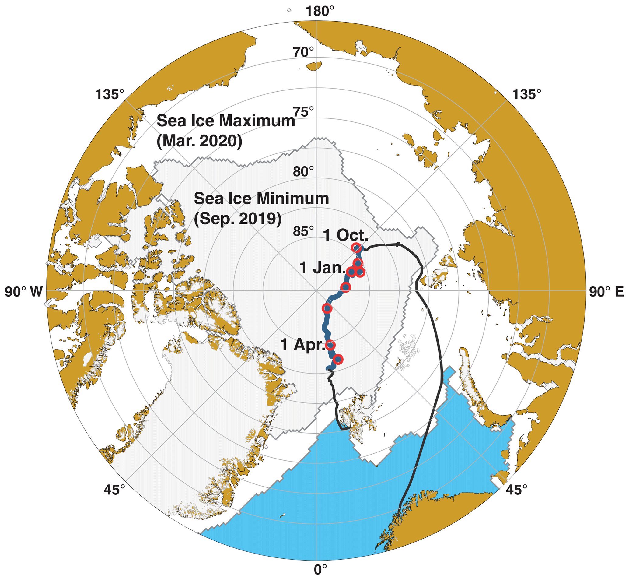
Figure 1Travel (black) and drifting (blue) route of the Polarstern from the beginning of October 2019 to the middle of May 2020. Each of the eight red circles marks the beginning of the next month. The map was produced with “ggOceanMaps” (Vihtakari, 2020) by using Sea Ice Index Version 3 data (Fetterer et al., 2020).
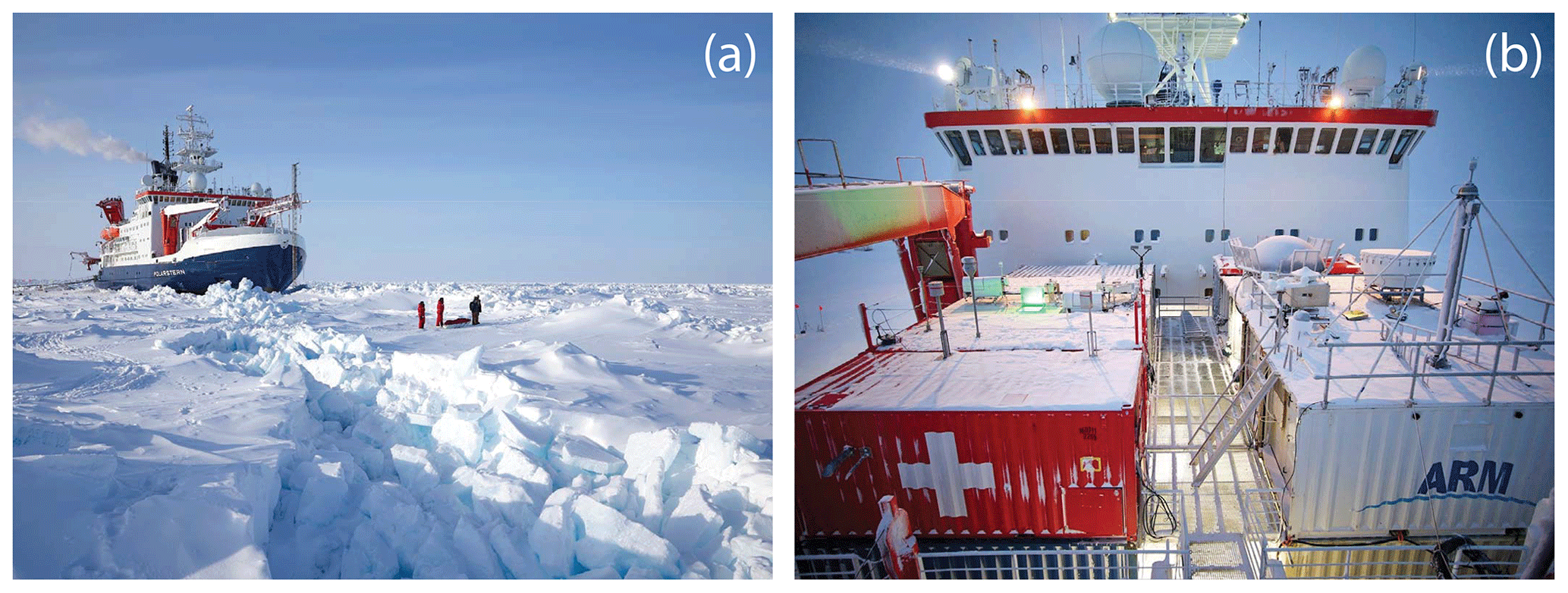
Figure 2(a) The Polarstern drifting in the Arctic ice on 10 April 2020 and (b) measurement containers for in situ aerosol monitoring (the first two containers on the left side and the first container on the right side) and for remote sensing of aerosols and clouds. The OCEANET-Atmosphere container of TROPOS is the third one on the left side (with the bright spot on the roof caused by green laser light). The ARM mobile facility (AMF-1) is shown on the right side. The photographs were taken by Michael Gutsche (CC-BY 4.0), AWI.
Figure 1 shows the track of the drifting Polarstern from October 2019 to May 2020. Each of the eight red circles along the Polarstern track indicates the beginning of a new month. The highest northern latitude with 88.6∘ N was reached around 20 February 2020. The Polarstern was at latitudes ≥85∘ N from the beginning of October 2019 to the beginning of April 2020. A photograph of the Polarstern in the ice- and snow-covered Arctic Ocean is shown in the left panel of Fig. 2 together with a photograph of the main ship-based MOSAiC atmospheric measurement platforms aboard Polarstern (right panel in Fig. 2). Six containers for in situ aerosol monitoring and for active remote sensing of aerosols and clouds with lidars and radars were deployed on the front deck of the research vessel. The ARM mobile facility AMF-1 on the right side consists of three portable shelters containing a baseline suite of instruments and communication and data systems.
The OCEANET-Atmosphere container of the Leibniz Institute for Tropospheric Research (TROPOS), routinely operated aboard Polarstern since 2009 (Kanitz et al., 2011, 2013; Bohlmann et al., 2018; Yin et al., 2019; Baars et al., 2020) is the third one on the left side of the container spots. Besides continuous observations with our multiwavelength Raman lidar (installed inside the air-conditioned container with specially designed roof window for optimum laser-beam transmittance and sampling of backscattered photons), two microwave radiometers for water vapor and cloud liquid-water measurements (one by the University of Cologne), two photometers for aerosol optical thickness (AOT) observations (one by the University of Lille), and a two-dimensional disdrometer were operated for ice crystal morphological studies. The TROPOS equipment was already aboard Polarstern 2 years ago and involved in the Arctic field campaign PASCAL (Physical feedbacks of Arctic boundary layer, Sea ice, Cloud and AerosoL) (Wendisch et al., 2019; Griesche et al., 2020, 2021).
2.1 Lidar instrument and operational details
Two advanced lidar instruments, the multiwavelength Raman lidar Polly (POrtabLe Lidar sYstem) (Engelmann et al., 2016) and a high spectral-resolution lidar (HSRL) (Eloranta, 2005), were operated continuously aboard the drifting Polarstern during the MOSAiC expedition. These two lidars are complementary regarding their capabilities. While the multiwavelength Raman lidar delivered detailed spectrally resolved optical properties of the aerosol in the Arctic and retrieval products regarding microphysical and cloud-relevant aerosol properties from October to March, i.e., during nighttime conditions, the single-wavelength HSRL is of advantage during the summer half year (when Raman lidar observations are of limited use) and allows us to measure profiles of the climate-relevant particle extinction coefficient at 532 nm wavelength even during sunlight conditions. Both lidar systems are polarization lidars and thus permit detailed monitoring of cloud phase and thus of liquid-water, mixed-phase, and ice clouds and morphological features (sphericity) of aerosol particles.
The MOSAiC expedition for the first time provided the unique opportunity to perform lidar observations north of 85∘ N over the entire winter half year 2019–2020. This part of the central Arctic is not covered by any other lidar measurement, neither by observations with the spaceborne CALIPSO lidar (only up to 81.8∘ N) nor by measurements of the ground-based Arctic lidar network (Nott and Duck, 2011). Thus, we add a new data set to the global aerosol database. Di Biagio et al. (2018) were the first to run lidars (mounted on an ensemble of autonomous drifting buoys) in the central Arctic, even north of 82∘ N, to perform year-round aerosol profiling, including the winter half year of 2015–2016. These measurements together with respective CALIPSO lidar observations are used in our contrasting analysis regarding the aerosol conditions during the MOSAiC year 2019–2020 and the year 2015–2016 characterized by unperturbed aerosol conditions (Ohneiser et al., 2021).
The setup and basic technical details of the Polly instrument are given in Engelmann et al. (2016), Hofer et al. (2017), and Jimenez et al. (2020b). Polly belongs to the lidar network PollyNET (Baars et al., 2016), which is part of the European Aerosol Research Lidar Network (EARLINET) (Pappalardo et al., 2014) organized within the Aerosols, Clouds and Trace gases Research InfraStructure (ACTRIS) project (ACTRIS, 2020). The lidar transmits linearly polarized laser pulses at 355, 532, and 1064 nm with a pulse repetition rate of 20 Hz. All laser beams point to an off-zenith angle of 5∘ to avoid a bias in the observations of the optical properties of mixed-phase and cirrus clouds caused by strong specular reflection by falling and then frequently horizontally aligned ice crystals (Noel and Sassen, 2005; Noel and Chepfer, 2010; Avery et al., 2020).
The receiver unit consists of a near-range receiver part, optimized to provide aerosol and cloud optical properties from 120 m to several kilometers above the surface, and a far-range receiver part which permits accurate aerosol and cloud profiling from about 800 m to 30–40 km height. Thirteen receiver channels are available to collect the following lidar return signals: elastically backscattered photons at the three laser wavelengths, the cross-polarized signal components at 355 and 532 nm at two different FOVs, the vibrational Raman signals of nitrogen at 387 and 607 nm, and those of water vapor at 407 nm. All signals are measured with photon-counting photomultipliers and stored with 30 s of resolution. We introduce “cross” and “co” to indicate the plane of polarization orthogonal and parallel to the plane of linear polarization of the transmitted laser pulses.
The recently introduced and implemented dual-FOV polarization lidar option (Jimenez et al., 2020a, b) permits the measurement of the cross and total (cross-polarized + co-polarized) signal components at 532 nm at two different FOVs. The dual-FOV lidar technique enables us to determine multiple scattering by droplets in liquid-water-dominated cloud layers and to retrieve from this multiple scattering information cloud microphysical properties (e.g., effective droplet size and cloud extinction coefficient) (Jimenez et al., 2020a). The method is based on the measurement of two volume linear depolarization ratios at two different FOVs. The depolarization ratio is defined as the ratio of the cross-polarized to the co-polarized backscatter coefficient.
The Polly instrument is designed for automated continuous profiling of aerosols and clouds and thus was running around the clock. Well-defined breaks were necessary to exchange laser flash lamps, to run different calibration procedures, to check the full setup, and to perform an overall alignment of the Polly instrument. Five TROPOS lidar scientists took care of the OCEANET instrumentation over the 1-year MOSAiC expedition period.
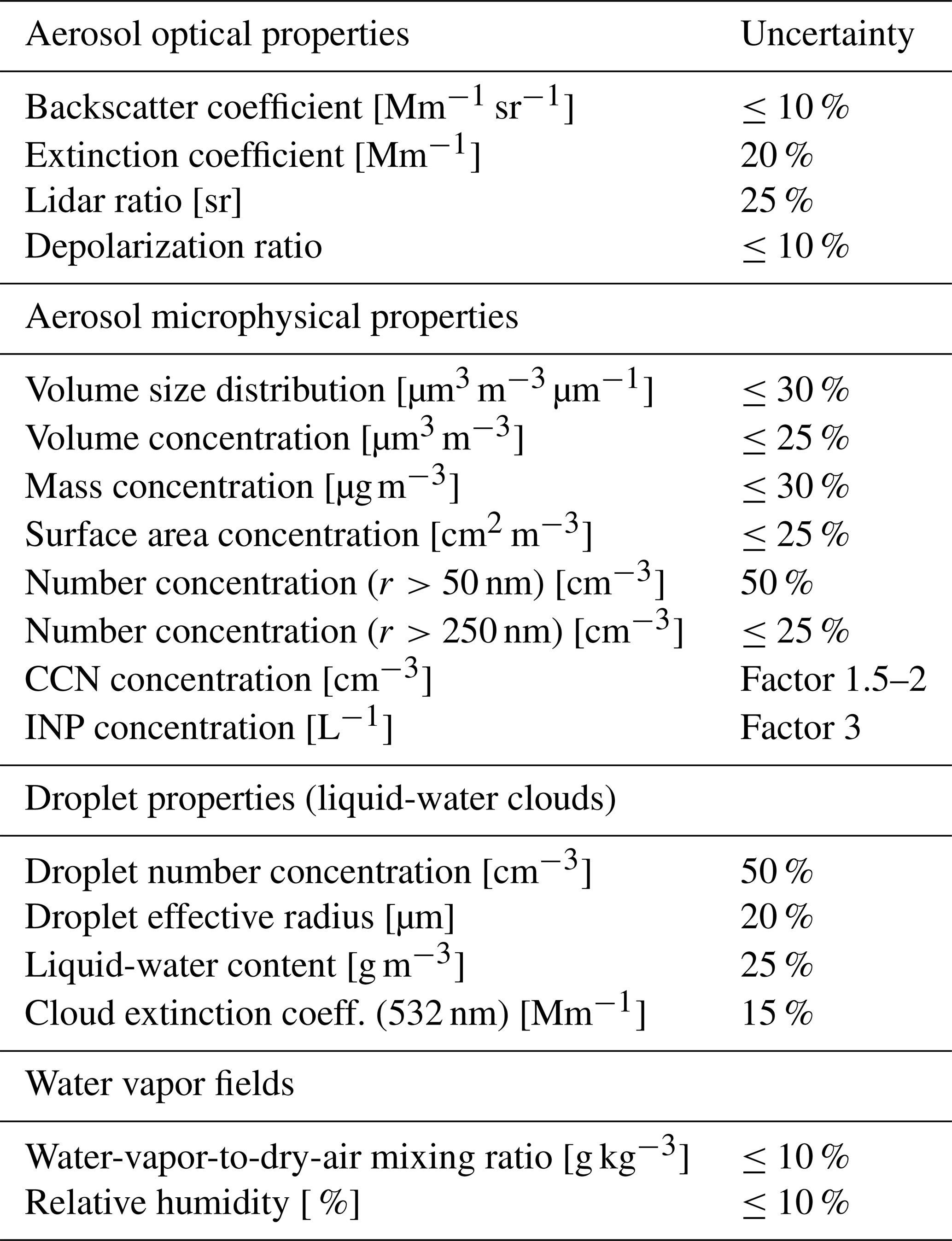
Table 1Overview of Polly observational products and characteristic (or typical) relative uncertainties in the determined and retrieved properties. Particle backscatter coefficients are measured at 355, 532, and 1064 nm, the other aerosol optical properties at 355 and 532 nm. r denotes aerosol particle radius.
2.2 Lidar products
The measurement and retrieval products obtained from the multiwavelength dual-FOV polarization and Raman lidar Polly are listed in Table 1. In addition, typical relative errors caused by signal noise and required input parameters in the data analysis are given in the table. The basic data analysis procedure to obtain aerosol and cloud optical properties is described by Baars et al. (2012), Baars et al. (2016), Hofer et al. (2017), Haarig et al. (2018), and Ohneiser et al. (2020, 2021). Height profiles of the particle backscatter coefficient at the laser wavelengths, of the particle extinction coefficient at 355 and 532 nm, respective extinction-to-backscatter ratio (lidar ratio) at 355 and 532 nm, the particle linear depolarization ratio at 355 and 532 nm, and the mixing ratio of water vapor to dry air by using the Raman lidar return signals of water vapor and nitrogen (Dai et al., 2018) can be determined. The aerosol Raman lidar method was applied to determine the particle backscatter and extinction profiles (Ohneiser et al., 2021).
The particle linear depolarization ratio (PLDR) is obtained from the measured volume linear depolarization ratio (VDR, depolarization ratio influenced by Rayleigh and particle depolarization of backscattered laser light). The PLDR can be used to discriminate spherical aerosol particles such as haze particles and liquid droplets, producing a PLDR close to zero, from non-spherical particles such as dust particles or ice crystals, causing a PLDR around 0.3 and typically >0.4 at 532 nm, respectively. In the case of Polly, the cross-polarized and total backscatter signals are measured. The specific approach to obtain the VDR from the Polly observations is described by Engelmann et al. (2016).
Although PollyNET delivers automatically calculated PLDR profiles, the lidar observations presented in this article and in the accompanying article of Ohneiser et al. (2021) were manually analyzed. To keep the uncertainties in the derived aerosol quantities at an acceptably low level of <10 % for the backscatter coefficients and depolarization ratios and of the order of 20 %–25 % for the particle extinction coefficients and lidar ratios, large vertical signal smoothing and regression window lengths of 500 to 2500 m and signal averaging times from 30 min to more than 10 h had to be applied. Fortunately during the winter half year, the nighttime conditions allowed us to apply the Raman lidar methods around the clock. More details are given in Ohneiser et al. (2021).
Auxiliary data are required in the lidar data analysis in the form of temperature and pressure profiles in order to calculate and correct for Rayleigh backscatter, extinction, and light-depolarization contributions to the measured lidar return signals. In the MOSAiC data analysis, we used the Polarstern radiosonde observations. As an important contribution to MOSAiC, radiosondes were routinely launched every 6 h (at 05:00, 11:00, 17:00, and 23:00 UTC) throughout the entire MOSAiC period (Maturilli et al., 2021).
The retrieval of aerosol microphysical properties such as particle volume, mass, and surface area concentration and estimates of cloud-relevant properties such as CCNC and INPC is performed by means of the POLIPHON (Polarization Lidar Photometer Networking) approach (Mamouri and Ansmann, 2016, 2017; Marinou et al., 2019; Ansmann et al., 2019, 2021). Lidar input data sets are the height profiles of the 532 nm backscatter coefficient and the PLDR. Hofer et al. (2020), for example, show the full set of height-resolved POLIPHON aerosol products in the cases of an 18-month Polly campaign in Dushanbe, Tajikistan, for central Asian aerosol. Alternatively to the POLIPHON method, we applied the multiwavelength lidar inversion technique (Müller et al., 1999, 2014; Veselovskii et al., 2002, 2012) to derive the microphysical properties of aerosol particles including the particle size distribution. The method of Veselovskii et al. (2002) is applied to MOSAiC smoke and Arctic haze observations to estimate layer mean microphysical properties in pronounced smoke and haze layers with sufficiently accurate backscatter coefficients at 355, 532, and 1064 nm and extinction coefficients at 355 and 532 nm.
Details of the analysis of the dual-FOV polarization lidar measurements can be found in Jimenez et al. (2020a, b). The method allows us to retrieve the cloud extinction coefficient and the effective radius of the droplets at a height of 50–100 m above cloud base and, in the next step, to calculate the liquid-water content (LWC, function of cloud extinction coefficient and effective radius) and cloud droplet number concentration from LWC by assuming a gamma size distribution.
Relative-humidity fields are obtained from the mixing-ratio measurements (Dai et al., 2018) (Raman lidar method) and temperature profiles measured with the Polarstern radiosondes. Quality checks of the continuously obtained water vapor fields were based on comparisons with the relative-humidity profiles obtained with radiosondes launched at 05:00, 11:00, 17:00, and 23:00 UTC.
A good knowledge of the tropopause height is important when profiling aerosol and cloud layers in the troposphere and stratosphere. The tropopause was computed from the MOSAiC radiosonde temperature and pressure profiles (Maturilli et al., 2021) by using the approach of the Global Modeling and Assimilation Office (GMAO), Goddard Space Flight Center, Greenbelt, Maryland, USA (GMAO, 2021). In this approach, the tropopause height zTP is found from the height profile of the difference αT(z)−log 10p(z) with α=0.03, temperature T (in Kelvin), pressure p (hPa), and height z (m). The tropopause pressure p(zTP) is defined as the pressure where the defined difference reaches its first minimum above the surface. If no clear minimum was found up to z=13 000 m over Polarstern, a tropopause height zTP was not assigned. The obtained tropopause heights agree well with the ones we obtained by applying the definition of the World Meteorological Organization (WMO, 1992) to the radiosonde temperature profiles and considering refinements in the determination described by Klehr (2012). In most cases, the GMAO approach delivered 20-80 m lower tropopause levels and produced fewer outliers.
The large spectrum of retrieved aerosol and cloud microphysical properties forced us to use any favorable opportunity for comparison with airborne in situ observations of these quantities in the framework of validation experiments in the past. These combined lidar and airborne in situ observations to characterize the quality of the retrieval products and to check the respective uncertainty ranges were usually available during large field campaigns. Regarding the aerosol microphysical properties, the comparisons showed that particle number concentrations, surface area, and volume and mass concentrations can be obtained with an uncertainty of 25 %–50 % (see Table 1) in cases with a clearly dominating aerosol type, e.g., in dense desert dust plumes or lofted wildfire smoke layers (Wandinger et al., 2002; Groß et al., 2016; Mamali et al., 2018; Haarig et al., 2019). The size distributions of aerosol particles can be precisely identified and estimated from multiwavelength lidar measurements in cases with a pronounced accumulation mode (Müller et al., 2004) as it is the case for aged wildfire smoke and aged Arctic haze.
Validation studies are especially valuable to characterize the potential of lidar to estimate cloud-relevant aerosol parameters such as CCNC and INPC. Comparisons with airborne in situ measurements showed that CCNC can be obtained with an uncertainty of about 30 % (inversion of multiwavelength data) to 50 % (conversion of the 532 nm extinction coefficient) when the aerosol type (and thus the typical aerosol size distribution) is known and about a factor of 2 if the aerosol type is not well known or mixtures of different aerosol types prevail (Düsing et al., 2018; Haarig et al., 2019; Georgoulias et al., 2020).
In a few efforts, the potential of lidar to deliver trustworthy INPC profile information was investigated based on simultaneous airborne in situ and lidar observations (Schrod et al., 2017; Marinou et al., 2019). These few attempts indicated that an INPC estimation is possible with an uncertainty within an order of magnitude. The large uncertainty is caused by the ice-nucleating particle (INP) parameterization used (taken from the literature) and not from the aerosol input parameters obtained from the lidar observations. In this field, much more coordinated field activities are needed. One alternative approach is to compare the derived INP concentrations with the estimated ice crystal number concentration from lidar–radar observations in so-called closure experiments. Good consistency in these closures indicates a high reliability of the selected INP parameterization (Marinou et al., 2019; Ansmann et al., 2019).
All these uncertainties in the aerosol retrievals can be considerably larger if the aerosol fraction of interest contributes to a minor part to the observed aerosol amount, i.e., when, for example, the interesting mineral dust fraction in Arctic haze is of the order of 10 %. For this reason, accompanying airborne in situ observations are always useful to better characterize the uncertainty range of the aerosol and cloud products gained from active remote sensing.
Concerning microphysical properties of liquid-water cloud layers (CDNC) and cirrus clouds (ICNC), validation studies based on aircraft–lidar comparisons are difficult because of the usually strong vertical and horizontal inhomogeneities in the cloud properties. Here, we make use of different, independent methods and techniques to derive estimates of CDNC and ICNC to check the quality of the retrievals (regarding CDNC, see, e.g., Jimenez et al., 2020b). Product evaluation efforts have been reported by Casenave et al. (2019) in the case of the retrieval of ice crystal microphysical properties from combined lidar–radar observations and were based on comparison with respective satellite retrievals or airborne in situ observations.
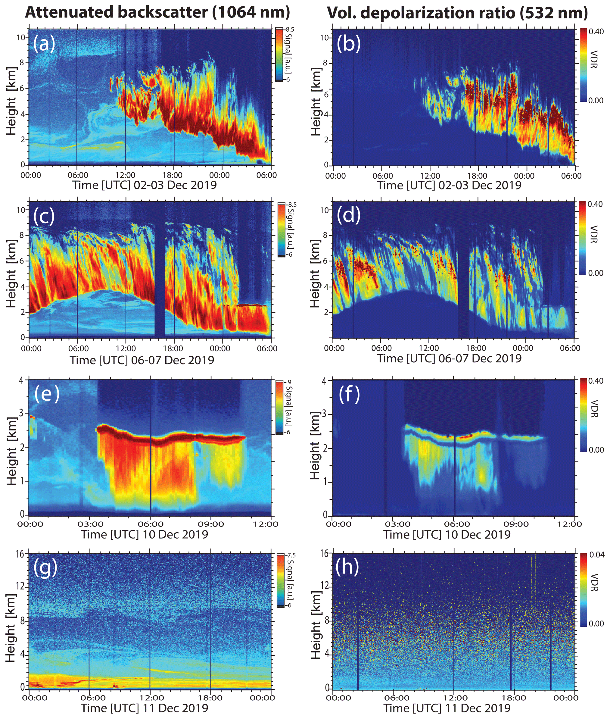
Figure 3Ice clouds, mixed-phase clouds, and aerosols monitored with Polly above the Polarstern from 2–11 December 2019. (a–d) Evolution of cirrus layers with strong virga embedded in wildfire smoke and Arctic haze, (e–f) development of a long-lasting mixed-phase altocumulus with shallow liquid-water layer at the top and ice virga below, and (g–h) Arctic haze (below 5 km height) and wildfire smoke (above 8 km) during clear-sky conditions. The range-corrected 1064 nm signal (left panels, in arbitrary units, a.u., logarithmic scale, the given exponents indicate the signal range) and the 532 nm volume linear depolarization ratio (VDR, right panels) are shown. Note that the color scales vary from panel to panel.
We begin with a series (snapshots) of typical aerosol and cloud scenes observed with our lidar during the winter months. According to Fig. 1, the Polarstern moved very slowly with the pack ice in December, January, and February and was mostly located between 86 and 88∘ N. The exceptionally strong polar vortex of 2019–2020 was well established during that time. Figure 3 shows a 10 d measurement sequence (2–11 December 2019). Complex features of aerosol layering, cirrus evolution (Fig. 3a–d), and mixed-phase cloud life cycles (Fig. 3e–f) were found. Clear, i.e., fog and cloud-free, periods occurred frequently as well and provided excellent conditions for a detailed characterization of Arctic haze and wildfire smoke.
The measured volume linear depolarization ratio (VDR) in the right panels of Fig. 3 allows us to precisely distinguish cirrus from layered mixed-phase clouds as explained above. Ice crystals cause large depolarization ratios (green to red colors in Fig. 3b, d, f), and, in contrast, liquid-water layers produce rather low depolarization ratios of around zero in Fig. 3f. The increase in the depolarization values with increasing penetration of the laser beam into the water cloud layer is caused by multiple scattering by the cloud droplets. This aspect is explained in more detail in Sect. 3.3. The depolarization ratio of aerosol particles was found to be generally small (Fig. 3h) in the free troposphere and stratosphere, which indicates spherical haze and smoke particles.
3.1 Wildfire smoke layer in the UTLS regime
Extreme and long-lasting wildfires in central and eastern Siberia, in closest neighborhood to the Arctic region, were most probably responsible for the UTLS smoke layer over the High Arctic in the winter half year of 2019–2020 (Johnson et al., 2021; Ohneiser et al., 2021). The main burning phase lasted from 19 July to 14 August 2019. In the absence of any pyrocumulonimbus (pyroCb) convection (Fromm et al., 2010) and thus of a very efficient and fast process to transport smoke into the UTLS height range, we hypothesize that the smoke was lifted by the so-called self-lifting process (Boers et al., 2010). Details are given in Ohneiser et al. (2021). In self-lifting processes, strong absorption of solar radiation by the black-carbon-containing smoke heats the air in lofted smoke plumes. The buoyancy created then forces the smoke plumes to ascend up to the tropopause (at around 10 km) within about 3–5 d according to our simulation studies (Ohneiser et al., 2021).
Once in the UTLS height range, smoke particles become quickly distributed over large parts of the Northern Hemisphere within a few weeks, as observed and documented for the first time in 2001 (Fromm et al., 2008) and recently confirmed after the record-breaking Canadian fires in the summer of 2017 (Khaykin et al., 2018; Baars et al., 2019). In the case of the strong Siberian fires, the smoke particles probably became quickly distributed over the entire Arctic region (as suggested by the satellite observations presented by Johnson et al., 2021) and then remained in the UTLS height range for months. The decay of smoke-related stratospheric perturbations usually takes more than a half year (Baars et al., 2019).
Besides the strong and long-lasting fires in Siberia, the Raikoke volcano erupted in June 2019 (Kloss et al., 2021; Vaughan et al., 2021). The amount of the emitted SO2 suggested that a stratospheric aerosol layer with a maximum 532 nm AOT of around 0.025 at latitudes >50∘ would form. It was further expected that the AOT would decrease to values of 0.01 over the High Arctic in autumn 2019 and to 0.005 during the winter months, as discussed in Ohneiser et al. (2021).
From the first days of the MOSAiC observations on, in late September 2019, we observed a pronounced and well-aged stratospheric aerosol layer with a backscatter maximum around or just above the tropopause, smooth internal structures, and clear wildfire smoke signatures. The 532 nm AOT was around 0.1 in autumn 2019 over the Polarstern and thus much higher than the expected sulfate AOT of 0.01. Further lidar observations at Leipzig (51.3∘ N, 12.4∘ E), Germany, and Ny-Ålesund, Svalbard (78.9∘ N, 11.9∘ E), Norway, indicated a strong increase in the stratospheric AOT in August 2019, probably as a result of the record-breaking Siberian fires and the spread of the smoke over large parts of the Northern Hemisphere.
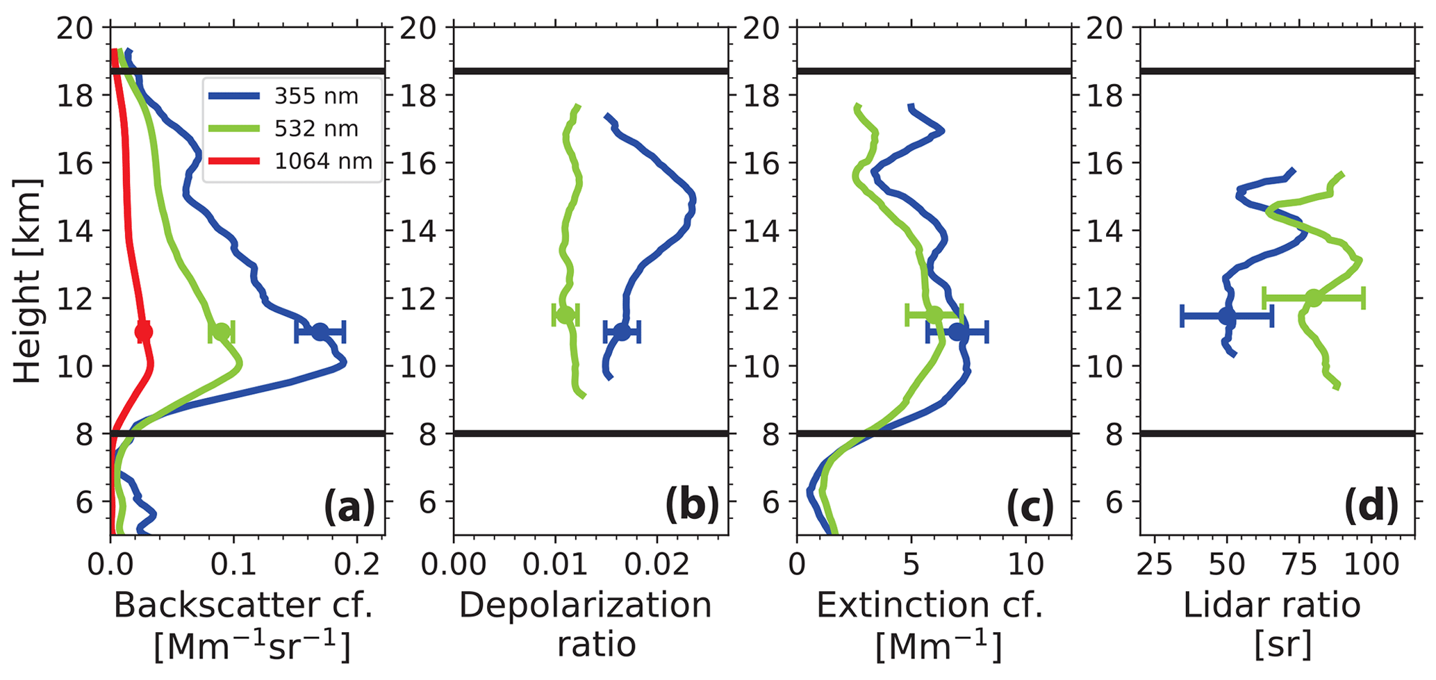
Figure 4Profiles of optical properties (24 h mean values) of the wildfire smoke layer on 11 December 2019. Base and top heights of the smoke layer are indicated by black horizontal lines. (a) Particle backscatter coefficient at three wavelengths, (b) particle linear depolarization ratio at 355 and 532 nm, (c) smoke extinction coefficient at 355 and 532 nm, and (d) respective smoke extinction-to-backscatter ratio (lidar ratio) are shown. All basic lidar signal profiles were smoothed with vertical window lengths of 500 m (backscatter, depolarization) and 2000 m (extinction, lidar ratio). Error bars indicate the estimated uncertainties (1 standard deviation). More details are given in Ohneiser et al. (2021).
Figure 4 presents the optical properties of the smoke layer as measured on 11 December 2019 (Fig. 3g and h). The Polarstern was at 86.6∘ N and 120.7∘ E at 12:00 UTC. The lidar observations were averaged over the entire day; thus 24 h mean height profiles are shown. The UTLS aerosol layer extended from 8 to more than 18 km height. The internal vertical structures were rather smooth. The layer base as indicated in Fig. 4 was determined by the altitude at which the 1064 nm backscatter coefficient started to increase with height. The smoke layer top was set to the height where the total-to-Rayleigh backscatter ratio at 1064 nm dropped below a value of 1.1.
A clear and unambiguous optical fingerprint for the presence and dominance of aged smoke particles (after long-range transport) is the unusual spectral dependence of the extinction-to-backscatter ratio L (Fig. 4d) together with a high 532 nm particle lidar ratio L532 typically exceeding 70 sr. L532 is much larger than the 355 nm lidar ratio L355, typically by more than 20 sr (Haarig et al., 2018; Ohneiser et al., 2021). Another smoke signature is the weak wavelength dependence of the particle extinction coefficient σ, expressed in terms of the extinction-related Ångström exponent Å. For the extinction profiles in Fig. 4c, Å is about 0.5. In the case of volcanic sulfate aerosol the Ångström exponent is typically clearly >1.0. Note that such an unambiguous identification of the wildfire smoke type is only possible with multiwavelength Raman lidars and high spectral-resolution lidars (Müller et al., 2014; Burton et al., 2015), which allow us to determine the particle extinction coefficient at several wavelengths.
The particle depolarization ratios at 532 nm (around 1 %) and at 355 nm (1 %–2 %) in Fig. 4b were very low. Such low values are indicative of spherical particles. We hypothesize that the comparably slow ascent (over several days) of the smoke particles up to the UTLS regime over Siberia in the summer of 2019 allowed the smoke particles to complete the aging process in the humid troposphere (with high levels of condensable gases). At the end of the particle aging process, the majority of the smoke particles showed a spherical core–shell structure and thus caused the low particle depolarization ratios. In contrast, in the case of pyroCb-related ascents (fast lifting within 30–90 min up to the tropopause) there is no time for particle aging. Then, the particles widely keep their original, non-spherical shapes and thus produce large depolarization ratios of about 20 % at 532 nm.
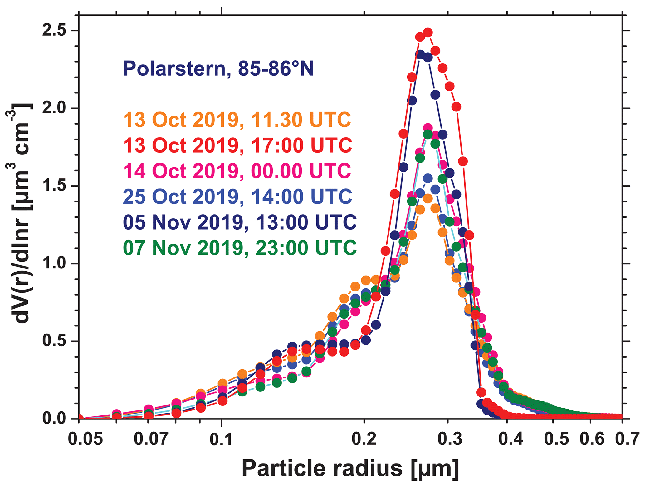
Figure 5Size distributions of the stratospheric smoke particles retrieved from the multiwavelength lidar observations on 5 d in October and November 2019. A narrow accumulation mode with particle sizes (diameters) from 400 to 1000 nm and a weak Aitken mode to the left are typical for aged wildfire smoke particles.
Figure 5 presents several volume size distributions of the smoke particles. The volume size distributions were obtained from the Polly observation by applying the lidar inversion method to the layer mean three backscatter and two extinction coefficients (Veselovskii et al., 2002). As typical for aged wildfire smoke, a well-defined accumulation mode was found. A distinct coarse mode was absent. The findings agree well with in situ observations of aged smoke transported over long distances (Fiebig et al., 2003; Petzold et al., 2007; Dahlkötter et al., 2014).

Figure 6(a) Overview of Polly observations of the UTLS smoke layer (colored bars from base to top, one bar per day) for the winter half year (October 2019 to April 2020). Observational gaps between bars are caused by opaque low-level clouds and fog. The colors in the bars provide information about the smoke particle extinction coefficient at 532 nm. The tropopause (black dots) separates the tropospheric from the stratospheric part of the smoke layer. Panel (b) shows 532 nm AOT of the smoke layer and estimated column mass concentration. (c) Smoke layer mean 532 nm particle extinction coefficient and estimated vertical mean particle mass concentration. The AOT and layer mean extinction values are computed from the profile of the backscatter coefficient multiplied by a 532 nm lidar ratio of 85 sr. AOT uncertainty is about 10 %–20 %. For comparison, background stratospheric extinction coefficients are expected to be of the order of 0.1–0.2 Mm−1 as observed over northern midlatitudes (Baars et al., 2019). More details are given in Ohneiser et al. (2021).
An overview of the smoke conditions during the MOSAiC winter half year (October to April) is presented in Fig. 6. Most of the time, the smoke layer was observed between 7 and 17 km height with the backscatter maximum just above the tropopause. A trend of downward movement of the layer is not visible. The maximum extinction coefficients (532 nm) decreased with time from values >10 Mm−1 in October and November to <5 Mm−1 in April 2020 (Fig. 6a).
The AOT in Fig. 6b was computed from the particle backscatter height profiles. The directly determined extinction profiles were too noisy, especially in the upper part of the smoke layer. The 532 nm backscatter coefficients were multiplied with the smoke mean lidar ratio of 85 sr (computed from all smoke observations measured during the winter half year) (Ohneiser et al., 2021). Subsequently, we integrated the extinction values between the smoke layer base and top heights as given in Fig. 4 to obtain the AOT. During the winter months, especially in January to February 2020, polar stratospheric clouds (PSCs) were frequently observed at the top and above the smoke layer, from 17 to 25 km height. We removed these PSC-affected parts from the height profiles of backscatter and extinction coefficients before we calculated the vertical column-integrated smoke optical properties. However, several weak PSCs developed within the smoke layer, and in this case, the backscatter and extinction contributions from these optically thin PSCs were not removed. The PSC-related uncertainty in the 532 nm AOT was estimated to be of the order of 5 % (Ohneiser et al., 2021).
In terms of the 532 nm AOT in Fig. 6b, the perturbation decreased from 0.05–0.12 in October and November to values of 0.03–0.06 in December to the middle of March and dropped to 0.01–0.02 in April 2020. Almost constant AOT conditions were observed from 10 December to 10 March. During that time period the strong polar vortex was established, dominated the airflow, even below the vortex, and controlled the horizontal and vertical exchange of gases and particles. As mentioned by Ohneiser et al. (2021), from mid December 2019 to mid April 2020, the weather pattern was rather stable and meridional air-mass exchange was widely suppressed. The vortex started to collapse around 20 April (Lawrence et al., 2020).
The 532 nm AOT of the volcanic sulfate aerosol was estimated to be about 0.01 in October 2019 and 0.005 during the winter months January and February 2020. According to the estimations in Ohneiser et al. (2021), the Raikoke aerosol fraction was always lower than 15 %.
The layer mean 532 nm smoke extinction coefficients in Fig. 6c (obtained from the ratio of AOT divided by the layer geometrical depth in Fig. 6a) were on the order of 10 Mm−1 in October, around 4–5 Mm−1 during the main winter months, and mostly ≤3 Mm−1 at the end of the lifetime of the smoke layer. From the measured layer mean extinction coefficients, mass concentrations of the smoke particles were derived (Ansmann et al., 2021) and ranged from 0.4–2 µg m−3 during the autumn and winter months. Note that AOT values for a clean stratosphere are around 0.001–0.002 (Sakai et al., 2016; Baars et al., 2019), and minimum extinction coefficients are of the order of 0.1–0.2 Mm−1. Minimum stratospheric mass concentrations (at midlatitudes) are close to 0.01–0.02 µg m−3 (Baars et al., 2019).

Figure 7Polar stratospheric cloud (PSC) from 17.5–22.5 km height on top of the smoke layer on 14 January 2020, 21:00-24:00 UTC. Three-hour mean particle backscatter coefficients and volume and particle linear depolarization ratio (PLDR) are shown. The optical properties are indicative of PSC Ib type. The 532 nm backscatter ratio (total-to-Rayleigh backscatter) peaks at 2.43 at 21.5 km height at about −86 ∘C. PSC optical thickness was 0.0125 at 532 nm (computed from backscatter values multiplied by a lidar ratio of 50 sr) (Kim et al., 2018). Horizontal gray lines show different temperature levels.
A PSC observation is shown in Fig. 7 at the end of this section. According to the PSC classification scheme (Achtert and Tesche, 2014), we observed type Ib PSCs. This type is made up of supercooled liquid ternary solutions that likely consist of H2SO4, HNO3, and H2O. In contrast to type Ia and II PSC particles (crystals) the liquid droplets of PSC type Ib only slightly depolarize incoming laser light. The temperature at PSC base height showed values of −78 ∘C, and at the backscatter maximum the MOSAiC radiosonde measured a temperature of −86 ∘C. We observed a much lower number of PSCs over the North Pole region (86 to 88.6∘ N) than the CALIPSO lidar (60 to 81.8∘ N) during the main PSC period from January to March (CALIPSO, 2020a, b).
3.2 Arctic haze vertical structures
The original and primary goal of the shipborne MOSAiC lidar measurements was to provide, for the first time, a height-resolved characterization of tropospheric aerosols and clouds over the North Pole region during the winter half year. Because of its importance for the climate and environmental conditions, Arctic haze has been intensively studied for more than 50 years (Law et al., 2014; Willis et al., 2018; Abbatt et al., 2019). However, knowledge about the vertical layering structures of these aged haze aerosols and about the composition and microphysical properties is still limited and mostly based on sporadic aircraft observations performed during field campaigns, preferably in spring (de Villiers et al., 2010; Quennehen et al., 2012; Ancellet et al., 2014). Furthermore, Ritter et al. (2016) presented a ground-based multiwavelength polarization Raman lidar study on Arctic haze in terms of backscatter, depolarization, and lidar ratios. The situation has improved since 2006 with the start of the CALIPSO mission (Di Pierro et al., 2013; Di Biagio et al., 2018; Yang et al., 2021).
As summarized by Willis et al. (2018), long-range transport of cold, polluted air masses from northern Eurasian source regions (mainly north of the Arctic front) prevails in winter and leads to the formation of Arctic haze with the highest mass concentrations in late winter and early spring. Such a low-level aerosol transport is missing in summer. Stohl (2006) pointed out that the winter transport of aerosols towards the High Arctic occurs at low heights. Long-transported aerosols may reach heights up to the middle troposphere (5–7 km height).
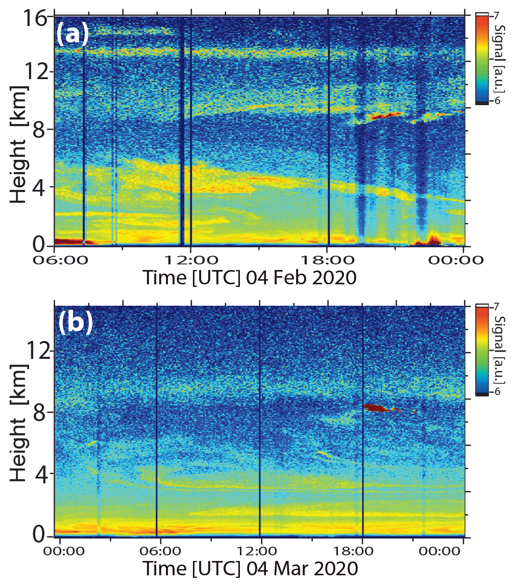
Figure 8Arctic haze (below 8 km height) and wildfire smoke (above 8 km height) over the North Pole region in late winter on (a) 4 February 2020 and (b) 4 March 2020. PSC layers are present as well at 13.5 and 15 km height on 4 February (pronounced yellow layers). The range-corrected 1064 nm signal is shown in arbitrary units (a.u., logarithmic scale).
In Fig. 8, we present two MOSAiC cases of Arctic haze observed on 4 February and 4 March 2020. The Polarstern was drifting with the ice at latitudes of 87.5∘ N (4 February) and 88.1∘ N (4 March). The most striking feature in both figures is that aerosol layers occurred almost everywhere within the troposphere and in the lower stratosphere. Remnants of PSCs were visible around 13.5–14 km height on 4 February 2020 (Fig. 8a). Temperatures were around −76 ∘C at 13.5 km height and thus sufficiently low to allow the formation of type Ia PSC (Achtert and Tesche, 2014; DeLand et al., 2020). Type Ia PSCs are thought to consist of nitric acid trihydrate (NAT) crystals and produce significant depolarization of backscattered laser light. Note that the Polarstern was fully below the strong polar vortex from the beginning of January to mid April 2020 (Ohneiser et al., 2021).
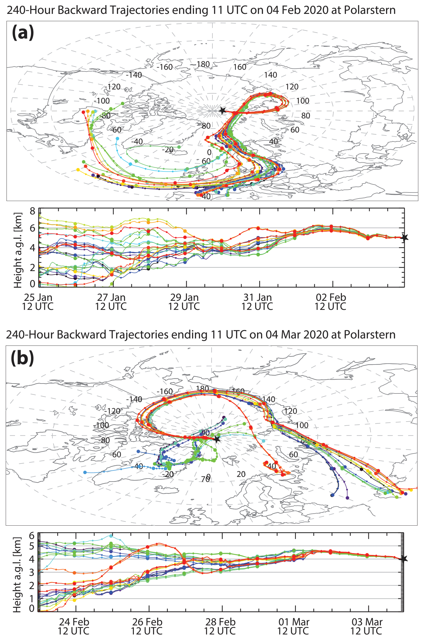
Figure 9(a) HYSPLIT 10 d ensemble backward trajectories arriving at the Polarstern on (a) 4 February 2020, 11:00 UTC arrival time, and on (b) 4 March 2020, 11:00 UTC arrival time (HYSPLIT, 2020; Stein et al., 2015; Rolph et al., 2017). According to Fig. 8, pronounced Arctic haze plumes were observed at the selected arrival heights of 5 km (4 February) and 4 km (4 March).
According to the backward trajectory analysis shown in Fig. 9, the aerosol pollution in the pronounced aerosol layers around 5 km (4 February, 11:00 UTC, Fig. 8a) and 4 km height (4 March, 11:00 UTC, Fig. 8b) originated from central and western European regions (4 February) and from Russia and the Black Sea area (4 March). The height-resolved trajectory analysis indicated that most of the aerosol circled around in the Arctic (at latitudes >70∘ N) for several days before crossing the Polarstern.
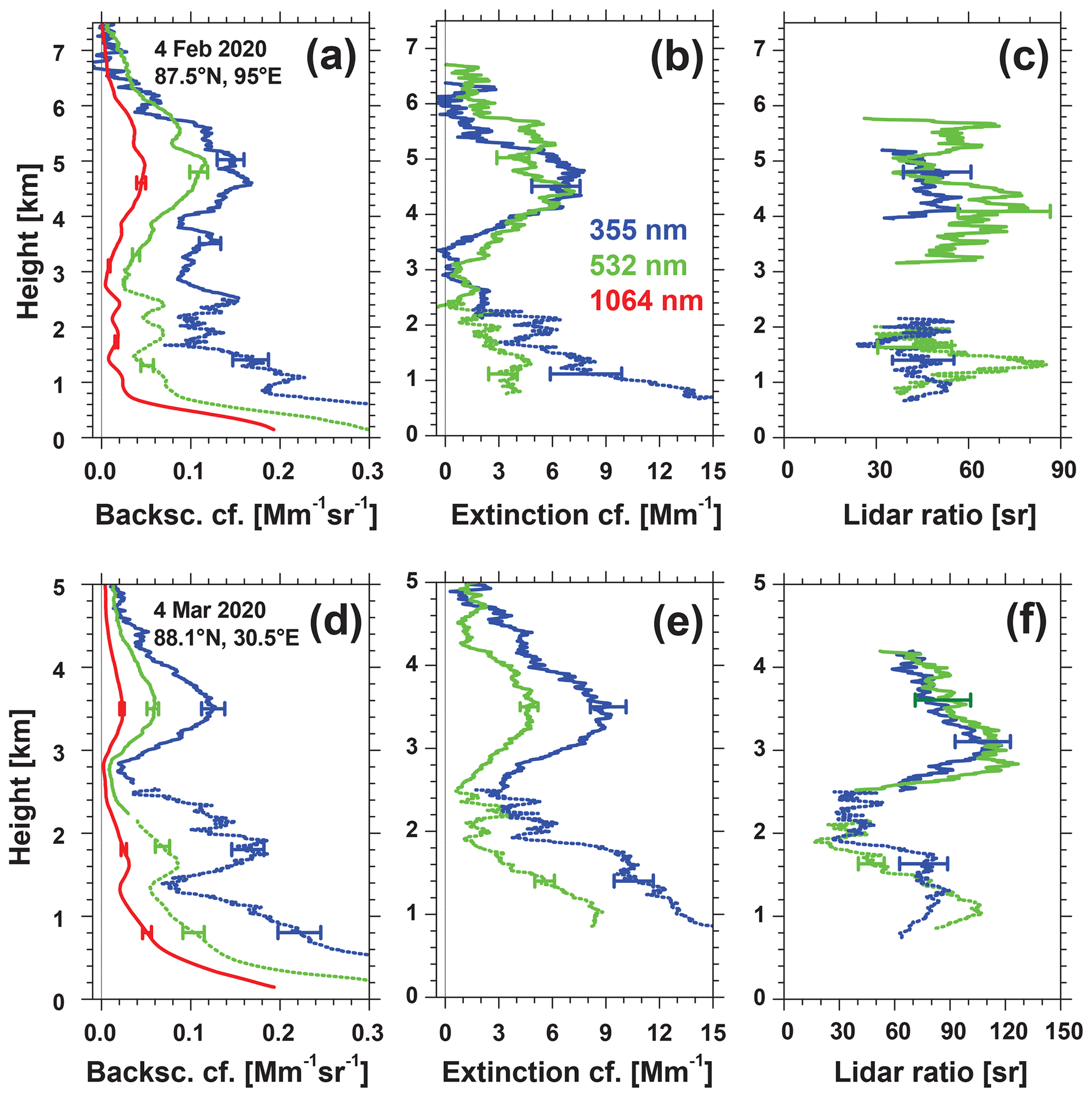
Figure 10Arctic haze backscatter, extinction, and extinction-to-backscatter ratios (lidar ratios). Mean profiles for 4 February 2020, 06:00–17:37 UTC, and for 4 March 2020, 00:00–17:45 UTC, are shown. A composite of near-range (dotted lines up to 2–3 km height) and far-range lidar observations (solid lines) is presented. Lidar signals are smoothed with vertical window lengths of 300 m (backscatter) and 900 m (extinction, lidar ratio). Error bars indicate the uncertainty (1 standard deviation) in the optical properties. The 532 nm AOT was 0.024 on 4 February (for heights up to 7 km) and 0.022 on 4 March (for heights up to 5 km).
In Fig. 10, the optical properties of Arctic haze for the two cases are illustrated. The figure shows 12 h (4 February) and 18 h (4 March) mean height profiles of the basic lidar products (backscatter, extinction, extinction-to-backscatter ratio). The long signal averaging times were needed to keep the signal-to-noise-related uncertainty below 10 % (backscatter coefficient), 20 % (extinction coefficient), and 25 % (lidar ratio). In both cases, we found a near-surface layer of up to about 2.5 km height and a separate lofted aerosol layer of up to 5 and 7 km height. A clear wavelength dependence of the backscatter and extinction coefficients was found on 4 March, as expected for fine-mode-dominated particles in the Arctic (Quennehen et al., 2012) consisting of a mixture of anthropogenic haze and fire smoke (Wang et al., 2011). The Ångström exponent for the extinction coefficient was around 1.7 in the lofted layer above 3 km height, and the lidar ratios were high with values of up to 100±15 sr. This is indicative of the presence of small, strongly light-absorbing particles.
On 4 February 2020 (Fig. 10a), the aerosol optical properties were less well defined, the extinction coefficients were almost equal at both wavelengths (355 and 532 nm), and the noisy lidar ratios at 532 nm were larger than at 355 nm in the lofted layer above 3 km height, which is typical for aged wildfire smoke as discussed in the foregoing section. The lidar ratios were lower than on 4 March; i.e., less absorbing particles were present. The volume depolarization ratios (not shown) were rather low in both cases and indicated the dominance of aerosol pollution. The 532 nm AOT was close to 0.025 (4 February, for the lowest 7 km height) and 0.02 (4 March, for the lowest 5 km) and thus considerably lower than the UTLS smoke AOT of about 0.04–0.05. The uncertainty in the tropospheric AOT values is about 20 %.
The values for the 532 nm extinction coefficients of 2–8 Mm−1 in the lower layer (up to 2.5 km height) and 1–7 Mm−1 in the lofted layer above 3 km height are in good agreement with CALIPSO lidar observations (Di Biagio et al., 2018; Yang et al., 2021). Di Biagio et al. (2018) showed 14 d mean and layer mean values of 2–8 Mm−1 (0–2 km layer), 2–10 Mm−1 (2–5 km), and 1–2 Mm−1 (5–10 km layer) measured in the area from 5–25∘ E (north of Svalbard) and 80–82∘ N in February and March 2015. Yang et al. (2021) analyzed 13 years of CALIPSO observations (June 2006 to December 2019) for the Arctic (entire area from 65 to 81.8∘ N) and found winter mean extinction values of 2–4 Mm−1 (2–6 km height) and around 2 Mm−1 (6–10 km height).
Our findings are also in good agreement with the results previously published and obtained during major field activities such as POLARCAT-IPY (Polar Study using Aircraft, Remote Sensing, Surface Measurements, and Models, of Climate, Chemistry, Aerosols, and Transport, International Polar Year) (Law et al., 2014) as well as during ARCTAS (Arctic Research of the Composition of the Troposphere from Aircraft and Satellites) (Wang et al., 2011). Both campaigns took place in the spring of 2008. Arctic haze was mostly found up to 7 km height. The aerosol composition was analyzed in great detail based on aircraft observations.
Wang et al. (2011) summarized and reviewed earlier Arctic observations and compared observations with model calculations and found that the ratio of black carbon (BC) to organic aerosol (OA) is high with values of 0.1–0.15 for aerosols advected from Russia. This aerosol is a mixture of anthropogenic haze (sulfate aerosol) and domestic, forest, and agricultural fire smoke (organic aerosol). Sulfate aerosol prevails in the near-surface air, whereas the OA fraction becomes comparably large in the free troposphere. Agricultural fires during spring (Europe, Asia) and flaring of natural gas (Russian oil industry) were found to be important sources for BC and OA particles. The fire smoke mixes with anthropogenic haze mainly from Asia during the long-range transport towards the central Arctic, beginning in late winter with peak occurrence in the spring season. Agricultural and forest fires produce ratios of typically <0.1, whereas anthropogenic haze may cause ratios >0.15.
3.3 Mixed-phase cloud evolution in Arctic haze
Two MOSAiC case studies of aerosol–cloud interaction are presented next. In this section, the evolution of a long-lasting mixed-phase altocumulus layer in Arctic haze within the lower free troposphere is discussed, and, in the next section, we present a cirrus development in the lower part of the UTLS wildfire smoke layer.
The mixed-phase cloud system was shown in Fig. 3e and f. The cloud layer was observed for more than 7 h over the Polarstern on 10 December 2019. The dark band in the depolarization ratio panel between 2–3 km height in Fig. 3f indicates the liquid-water-dominated cloud top layer. The increase in the depolarization ratio above the dark zone at the liquid cloud base is caused by multiple scattering by cloud droplets. Favorable conditions with cloud top temperatures around −28.5 ∘C at 2.6 km height (at 03:00 UTC) were given for heterogeneous ice formation via immersion freezing, i.e., ice nucleation on INPs immersed in the water droplets (Kanji et al., 2017). After nucleation in the cloud top layer, ice crystals grow fast to sizes of 50–100 µm within minutes (Bailey and Hallett, 2012) and immediately start to fall out. As visible in Fig. 3e and f, the crystals formed long virga below the shallow altocumulus layer. The ice crystals partly evaporated on the way down but partly reached the ground as precipitation. The liquid-water-dominated cloud top layer was not depleted at any time during the 7 h period.
About 40 long-lasting mixed-phase cloud events (ice-precipitating shallow altocumulus decks) with durations from 4–30 h were observed from October 2019 to March 2020. Because of their sensitive influence on radiative transfer and the water cycle, they have been the focus of research for more than 15 years (Verlinde et al., 2007; Mauritsen et al., 2011; Morrison et al., 2012; Paukert and Hoose, 2014; Loewe et al., 2017; Andronache, 2018; Eirund et al., 2019). However, because of the complexity of influencing meteorological and aerosol aspects, there are still many open questions concerning their long lifetime, especially of the longevity of liquid-water layers and thus of water droplets in the presence of ice crystals. MOSAiC contributes to this research field by means of combined lidar and radar observation.
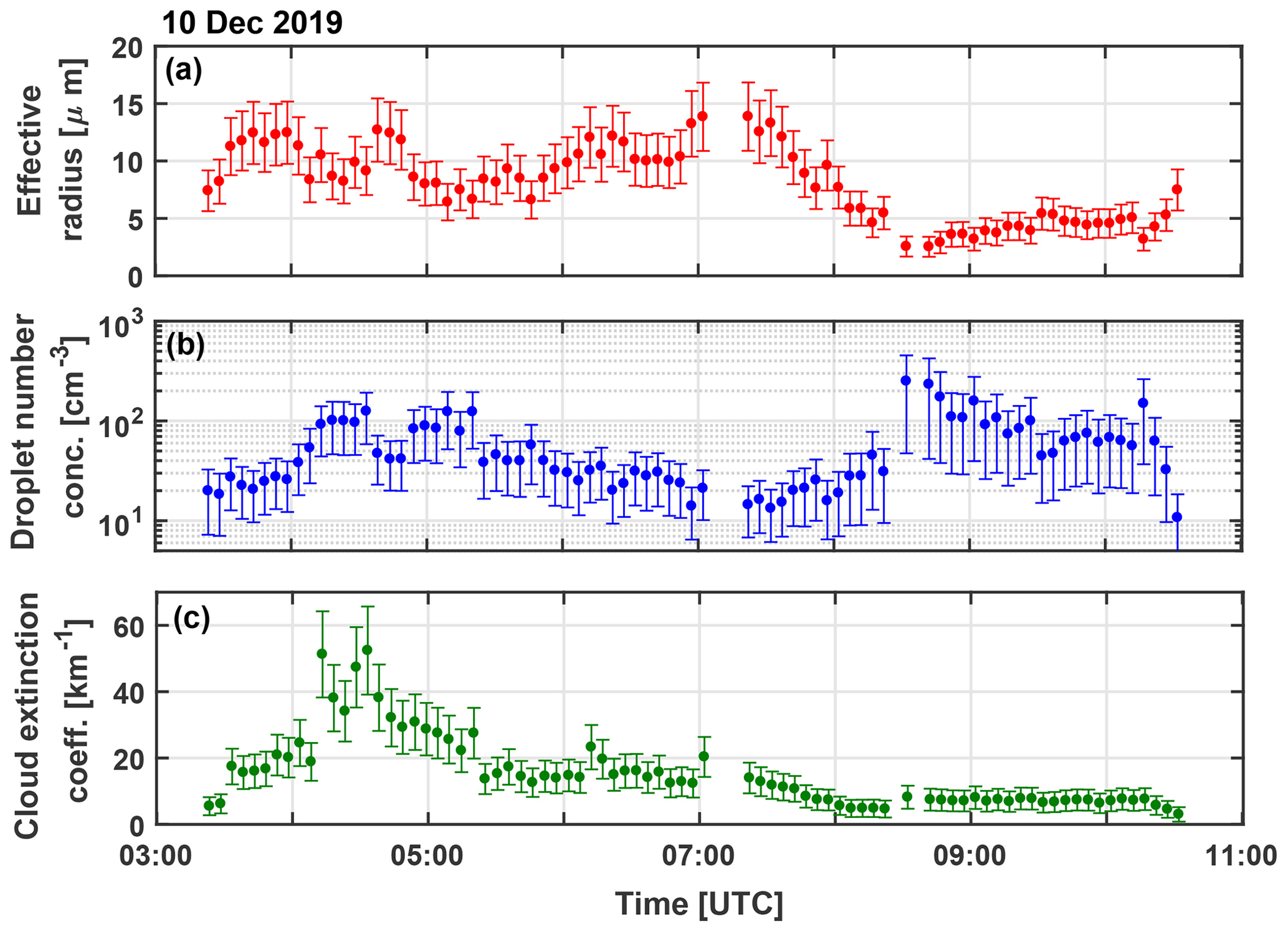
Figure 11(a) Effective radius of cloud droplets, (b) cloud droplet number concentration, and (c) 532 nm cloud extinction coefficient (single-scattering) at 75 m above cloud base of the altocumulus layer in Fig. 3e and f. The effective radius can be interpreted as the characteristic droplet radius. Error bars indicate the uncertainty. The cloud properties were retrieved by means of the recently introduced dual-FOV polarization lidar technique.
We applied our recently developed dual-FOV polarization lidar method (Jimenez et al., 2020a, b) to derive the microphysical properties of liquid-water droplets in the cloud top layer. The results are shown in Fig. 11. The dual-FOV lidar technique was originally designed for pure liquid-water cloud observations but can be applied to mixed-phase clouds as long as backscattering by ice crystals is negligible compared to droplet backscattering in the cloud top layer. This condition holds here with ice crystal backscatter coefficients of 5–10 in the virga (not shown) and thus probably also in the cloud top layer with droplet backscatter coefficients of the order of 700 (not shown). In the case of crystal-to-droplet backscattering of 0.01, the contribution of ice crystals to the observed multiple scattering features, from which the microphysical properties of the droplets are retrieved, can be ignored. Note that the method delivers the time series of droplet effective radius, CDNC, and cloud extinction coefficients in Fig. 11 for the height of 75 m above cloud base. Thus, the properties of freshly formed droplets are mainly observed.
As can be seen, the retrieved CDNC values were around 20 cm−3 in the beginning and around 100 cm−3 in the cloud base region later on. With increasing CDNC the effective radius (a characteristic droplet size) decreased and vice versa as expected when assuming a constant water vapor reservoir for droplet nucleation. The cloud extinction coefficient showed typical values from 10–20 km−1 in the first half of the cloud lifetime. Uncertainties in the lidar products are indicated by error bars (1 standard deviation) and are of the order of 20 %–25 % (cloud extinction coefficient, droplet effective radius) and 50 % (CDNC).
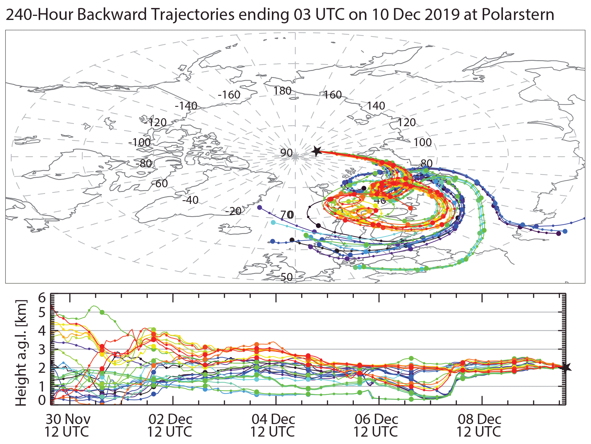
Figure 12HYSPLIT 10 d ensemble backward trajectories arriving at 2 km height above the Polarstern (black star) on 10 December 2019, 03:00 UTC. Thin and thick symbols indicate 6 and 24 h time steps, respectively.
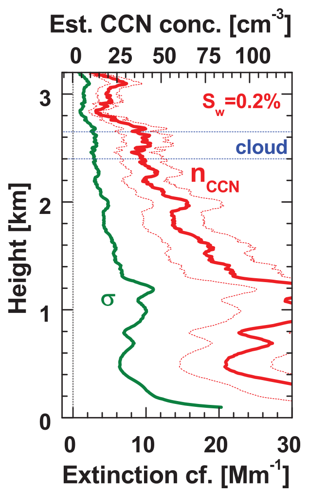
Figure 13Aerosol observation on 10 December 2019, 02:15–02:45 UTC, just before the altocumulus layer was detected over the lidar station (see Fig. 3e). The profile of the 532 nm extinction coefficient σ is estimated from the backscatter coefficient profile (assuming a lidar ratio of 30 sr obtained from the Raman lidar observations). The estimated CCN concentration (nCCN for a water supersaturation of 0.2 %) is obtained from the multiwavelength lidar data analysis (inversion technique, see text for more details). The thin red dotted lines show the assumed uncertainty range of ±30 %. Cloud base and top heights of the altocumulus layer at 03:30 UTC are indicated by horizontal lines.
In the next step, we wanted to know how many cloud condensation nuclei (CCN) were available. According to the HYSPLIT backward trajectories in Fig. 12, the altocumulus layer developed in aged Arctic haze, originating from northern parts of Europe. In order to estimate the CCN concentration (nCCN in Fig. 13) just below the altocumulus layer, the lidar observations in clear skies (before 03:00 UTC) were analyzed. The result is shown in Fig. 13. In this specific measurement, we used the multiwavelength Raman lidar technique and applied the lidar inversion method (see Sect. 2.2) (Veselovskii et al., 2002) to a set of three backscatter and two extinction coefficients. Here, the data analysis was based on the mean backscatter and extinction values (for the height range from 1500–2000 m height). The goal was to obtain (a) a value for the mean aerosol particle number concentration n50 (particles with radius >50 nm) and (b) a ratio of n50 to the 532 nm backscatter coefficient. We assumed that the obtained n50 value is a good estimate for nCCN (for a supersaturation level of Sw=0.2 %) (Mamouri and Ansmann, 2016). By using the obtained ratio of n50 to the 532 nm backscatter coefficient, the entire profile of the 532 nm particle backscatter coefficient was converted into a nCCN profile as shown in Fig. 13. The profile of the 532 nm particle extinction coefficient shown in Fig. 13 was obtained by multiplying the backscatter coefficients with a lidar ratio of 30 sr as obtained from the backscatter and extinction Raman lidar observations. The dashed nCCN curves indicate an uncertainty of 30 % in the n50 and nCCN estimation. The uncertainty of 30 % is much lower than indicated in Table 1. The uncertainty in the Table 1 holds in the case of the simpler conversion method (Mamouri and Ansmann, 2016).
Figure 13 shows that the estimated nCCN values of 25–55 cm−3 around 2500 m height were in the same range as the numbers of the retrieved CDNC (10–40 cm−3 in Fig. 11b) in the beginning of the cloud evolution. The actual updraft characteristics at cloud base determine the actual supersaturation levels. Strong updrafts may produce water supersaturation levels exceeding 0.5 %. Then the CCNC values are 50 %–100 % larger than our estimates in Fig. 13 as discussed in Mamouri and Ansmann (2016). All in all, we can conclude that the lidar observations provide a clear link between low aerosol particle concentration and therefore low CDNC in the mixed-phase cloud top layer. The aerosol conditions controlled the microphysical properties in the liquid-water-dominated cloud top layer.
In order to better understand the entire role of aerosol particles in the evolution of mixed-phase clouds, we also estimated the ICNC in the virga from combined lidar–radar observations (Bühl et al., 2019) and the INPC for the cloud top temperature of −28.5 ∘C from the 532 nm extinction coefficient in Fig. 13 (Mamouri and Ansmann, 2016).
Without going into too much detail, weakly enhanced PLDR values above 2 km height indicated a minor contribution of mineral dust particles (about 5 %) to the overall Arctic haze backscatter coefficient. This finding is in good agreement with studies of Di Biagio et al. (2018) and Yang et al. (2021), who analyzed spaceborne and ground-based lidar observations in combination with backward trajectory analysis and concluded that mineral dust typically contributes to the continental aerosol mixtures in the lower and middle free troposphere in the Arctic that were transported over long distances. Dust is the most favorable although not the only relevant INP type in the case of immersion freezing at temperatures ∘C during the winter half year when biogenic and biological components are absent (DeMott et al., 2010; DeMott et al., 2015; Kanji et al., 2017, 2020; Schill et al., 2020a). We used the INP parameterization scheme of DeMott et al. (2015) to estimate the dust INP concentration for immersion freezing. Here, the particle number concentration n250 of dust particles with diameters >500 nm is an input parameter and obtained from the respective lidar observation of the dust-related 532 nm backscatter coefficient (Mamouri and Ansmann, 2016). The retrieval finally yielded INPC estimates in the range from 0.1–0.5 L−1 for the altocumulus top temperature of −28.5 ∘C. Uncertainties in the INPC estimates are of the order of a factor of 3 (i.e., within an order of magnitude). The main uncertainty source is the INP parameterization and not the retrieval of n250 values.
To obtain also an estimate for ICNC, we used the lidar observations of the 532 nm extinction coefficient in the first strong ice virga zone (04:00–05:00 UTC) below the liquid-water cloud layer together with radar reflectivity (8 mm wavelength) and Doppler information on the ice crystal fall speed spectrum in the virga from the AMF-1 KAZR (Ka-band zenith-pointing radar) (ARM-MOSAiC, 2021). These observations were compared with comprehensive model simulations of the lidar and radar observations as a function of ice crystal number concentration, size distribution, and shape (Bühl et al., 2019). The match between simulations and observations provide the range of retrieved ICNC values. In the case of the mixed-phase cloud we obtain 0.1–1.0 ice crystals per liter within the virga. Again, the retrieval uncertainty allows us to provide the order of magnitude of ICNC only.
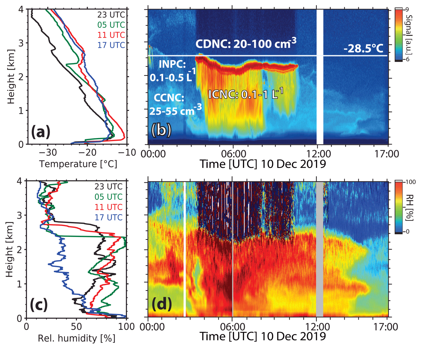
Figure 14Mixed-phase cloud closure study. (a, c) Profiles of temperature and relative humidity (over water) measured with four MOSAiC radiosondes launched at 23:00 UTC (9 December), 05:00, 11:00, and 17:00 UTC (10 December). (b) The 1064 nm range-corrected signal showing the mixed-phase cloud layer between 2 and 2.6 km height with ice virga below the main cloud layer, and (d) height–time display of Raman lidar observations of relative humidity. In (b), cloud-droplet number concentration (CDNC) as obtained from the dual-FOV lidar observations (during the 03:15–05:00 UTC time period), CCN and INP concentrations (CCNC, INPC) estimated from the lidar observations at 2.5 km height (CCNC) and at 2.6 km height (INPC, for the given cloud top temperature of −28.5 ∘C) in clear sky (02:15–02:45 UTC, i.e., before the cloud layer appeared), and ice crystal number concentration (ICNC, 04:00–05:00 UTC mean value) as estimated from combined lidar–radar observations are given as numbers. In (b), the 1064 nm signal is biased in the near range (<1000 m), especially during the strong virga backscattering periods.
Figure 14 summarizes our data analysis efforts and highlights the overall potential of our advanced aerosol/cloud lidar to contribute to cloud research. Since radiosondes were launched every 6 h (Fig. 14a and c) over the entire MOSAiC year, excellent conditions for a detailed lidar-based aerosol and cloud monitoring (Fig. 14b), including a coherent monitoring of the relative-humidity field (Fig. 14b), were given during the MOSAiC winter half year.
The temperature and relative-humidity (RHw) profiles measured with four radiosondes before, during, and after the cloud event indicate that the liquid-water-dominated cloud top layer was never thicker than a few 100 m. The cloud system developed in a warm and moist air mass and vanished when the moist air mass was replaced by very dry air (see 17:00 UTC radiosonde RHw profile in Fig. 14c). A strong drop in the relative humidity at all heights occurred around 15:00 UTC according to the lidar observations in Fig. 14d. The relative humidity (from lidar) is obtained from the Raman lidar observation of the specific humidity (water-vapor-to-dry-air mixing ratio) and radiosonde temperature profiles permitting the computation of the respective water-saturation-related specific humidity levels (Dai et al., 2018).
As mentioned above, favorable conditions for ice nucleation (via immersion freezing on dust particles) were given at cloud top temperatures of −28.5 ∘C in the beginning of the cloud lifetime and at around −25 ∘C later on. Strong ice crystal evaporation in the virga zone caused the strong moistening of the air mass below the main altocumulus deck after 03:00 UTC and also caused reduced crystal evaporation later on so that ice crystals could partly reach the ground as precipitation.
All estimated values for CCNC, CDNC, INPC, and ICNC are included in the lidar panel in Fig. 14b. We can summarize our observations as follows: during the early altocumulus development, the estimated CCNC values outside of the cloud were in a similar range to the estimated CDNC levels within the cloud as was also the case for the estimated INPC and ICNC levels. Thus, our data suggest that the estimated cloud active particle levels could be high enough to control the case-study cloud at given favorable moisture conditions and in the absence of other processes that might influence CDNC and ICNC levels (e.g., secondary ice formation, crystal-crystal collision and aggregation processes, or droplet collision and coagulation events). This hypothesis would be in line with numerous other Arctic studies that have previously observed this phenomenon (e.g., Mauritsen et al., 2011). However, higher-resolution in-cloud microphysical data are required to verify this lidar-based hypothesis.
It is worth mentioning that the estimated INP concentrations of 0.1–0.5 L−1 in Fig. 14b are also in line with previous Arctic in situ observations at similar temperatures. The measured INP values ranged from 0.001 to around 2.5 L−1 for temperatures from −25 to about −28 ∘C (Mason et al., 2016; Creamean et al., 2019; Wex et al., 2019; Hartmann et al., 2020). As part of the MOSAiC data analysis, we plan to analyze many winter as well as summer altocumulus events and thus cloud formation under contrasting aerosol conditions to obtain an improved view of the role of aged aerosol pollution that has been transported over long distances in the evolution of mixed-phase clouds in the High Arctic.
3.4 Cirrus evolution in wildfire smoke
According to a study of Barahona et al. (2017), Arctic ice clouds tend to form almost exclusively by heterogeneous ice nucleation with a contribution of only 10 % by homogeneous freezing. MOSAiC now offers an excellent opportunity to investigate the potential impact of aged wildfire smoke particles on cirrus formation. More than 50 cirrus systems developed in the upper troposphere in a smoke-influenced environment during the winter half year. The importance of such a smoke impact study arises from the fact that OA, besides dust and marine particles, is ubiquitous in the atmosphere (Schill et al., 2020b). However, in contrast to dust and marine particles the INP potential of OA is not well understood. Scarce field data are the main reason for the lack of clarity and knowledge.
Because of the complex chemical, microphysical, and morphological properties of aged fire smoke particles, which can occur as glassy, semi-liquid, and liquid aerosol particles, the development of smoke INP parameterization schemes is a crucial task. Smoke particles from forest fires are largely composed of organic material (organic carbon, OC) and, to a minor part, of BC. The BC mass fraction is typically <5 % (Dahlkötter et al., 2014; Yu et al., 2019). Biomass burning aerosol also consists of humic like substances (HULISs) which represent large macromolecules. The particles and released vapors within biomass burning plumes undergo chemical and physical aging processes during long-range transport such as coagulation, condensation, and heterogeneous reactions, resulting in changes in their morphological characteristics (size, shape, and internal structure) and mixing state.
Our knowledge on the potential of smoke particles to serve as INP is mainly based on laboratory and field studies of the ice nucleation potential of fresh smoke (with a focus on black carbon or soot particles) (Petters et al., 2009; Twohy et al., 2010; Prenni et al., 2012; McCluskey et al., 2014; Levin et al., 2016; Kanji et al., 2020; Schill et al., 2020a). However, aged smoke in the upper troposphere (at cirrus level, several days, weeks, or months after emission) has fundamentally different properties to the ones of wildfire particles emitted just a few minutes to hours ago (Reid and Hobbs, 1998; Fiebig et al., 2003; Dahlkötter et al., 2014). As China et al. (2015) pointed out, freshly emitted soot or BC particles are typically hydrophobic, lacy fractal-like aggregates. During transport, lacy soot undergoes compaction upon humidification. Schill et al. (2020b) mention that, during the aging process, the particles can also accumulate secondary sulfate mass from condensation of gaseous sulfuric acid that is present in the background atmosphere.
In this section, we present a MOSAiC cirrus case study to illuminate, for the first time, the potential of aged wildfire smoke to influence ice formation in the upper troposphere. An overview of organic particles, their complex properties, and ice-nucleating efficacy is given in the review article of Knopf et al. (2018). It is assumed that aged smoke particles show an almost perfect spherical core–shell structure and that the ability of smoke particles to serve as INP mainly depends on the organic material (OM) in the shell of the coated smoke (or soot) particles. At low temperatures, e.g., in the UTLS region, where the atmospheric temperature can be as low as 180 K, it is conceivable that the particles are in a glassy state. Aerosol particles serving as INPs usually provide an insoluble, solid surface that can facilitate the freezing of water (Knopf et al., 2018). Deposition ice nucleation is defined as ice formation occurring on the INP surface by water vapor deposition from the supersaturated gas phase. When the supercooled smoke particle takes up water or its shell deliquesces, immersion freezing can proceed, where the INP immersed in an aqueous solution can initiate freezing (Knopf et al., 2018; Berkemeier et al., 2014). If the smoke particle becomes completely liquid (and no insoluble part within the particle is left), homogeneous freezing will take place at temperatures below 235 K (Koop et al., 2000).
Our MOSAiC observation was performed on 6 December 2019. As shown in Fig. 3c and d, a long-lasting cirrus event was monitored. The full cirrus lifetime was about 36 h. Large virga of falling ice crystals permanently removed ice crystals from the cloud top region where they were nucleated. The cirrus system developed in the lower part of the UTLS smoke layer. The bow-like feature of the lower boundary of the extended virga zone was caused by a high-pressure ridge (with dome-like temporal evolution of the influenced height range). The ridge crossed the Polarstern during this day and was characterized by a warmer and very dry air mass in the lowest few kilometers of the troposphere. Ice crystals falling into this dry air mass immediately evaporated.
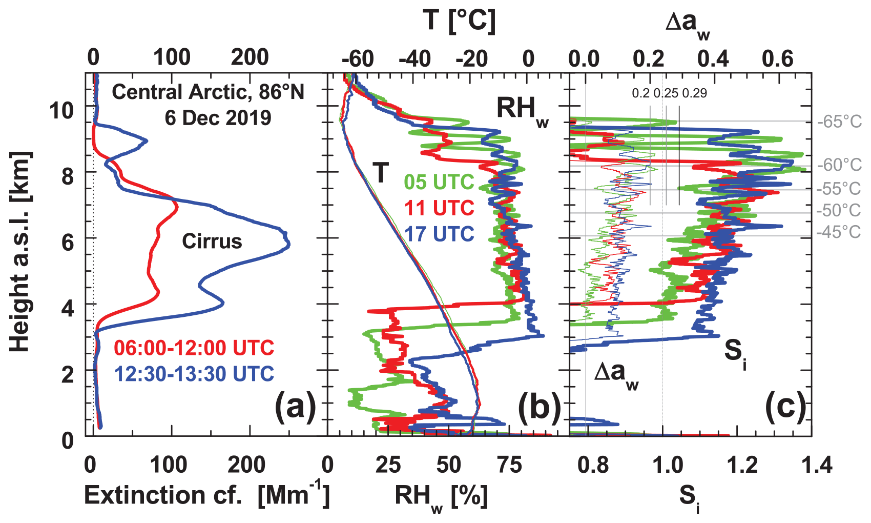
Figure 15(a) Temporally averaged (mean) cirrus extinction coefficient σ (532 nm) for two observational periods from 06:00–12:00 UTC (red) and from 12:30–13:30 UTC (blue, see Fig. 3c), (b) profiles of temperature T and relative humidity RHw (over water) observed with radiosondes launched at 05:00, 11:00, and 17:00 UTC on 6 December 2019, and (c) water activation criterion Δaw and ice supersaturation Si computed from the temperature and water vapor observations shown in (b). The water activation criterion Δaw is the difference between the observed RHw (in decimal numbers) and the ice-saturation-related RHw value (for the observed temperature). In (c), different temperature levels are indicated by thin horizontal lines and Δaw values of 0.2, 0.25, and 0.29, required to initiate ice nucleation, are shown as vertical line segments.
Figure 15 shows the mean cirrus layer structures measured from 06:00–12:00 UTC and in the early afternoon (12:30–13:30 UTC) together with the meteorological conditions in terms of air temperature, relative humidity, and ice supersaturation measured with three MOSAiC radiosondes at about 05:30, 12:30, and 17:30 UTC (30 min after launch). Very constant meteorological conditions were found from about 4 km up to cirrus top at 8–9.5 km height. Temperatures were below −40 ∘C at heights >5.5 km so that the development of high-altitude liquid-water layers was impossible. Clear ice supersaturation conditions (Si>1.1) were present in the upper part of the cirrus system.
It is worth mentioning that equilibrium in ice supersaturation conditions as observed in the extended virga zone over the whole day (Fig. 15c) is a sign of a low crystal number concentration (<35 L−1) (Murray et al., 2010). Such a low amount of ice crystals is not able to quench the supersaturation, which is in turn indicative of heterogeneous ice nucleation. Homogeneous freezing would produce crystal concentrations of >500 L−1 so that equilibrium at ice saturation level would occur within a short time period. Figure 15 is further discussed below.
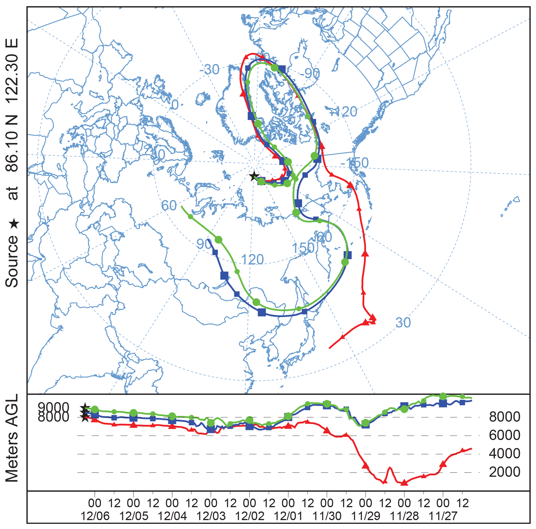
Figure 16HYSPLIT 10 d backward trajectories arriving at 8, 8.5, and 9 km height above the Polarstern (black star) on 6 December 2019, 06:00 UTC. Thin and thick symbols indicate 6 and 24 h time steps, respectively.
The HYSPLIT backward trajectories in Fig. 16 indicate that the humid air mass, in which the cirrus started to form, originated from the remote northern Pacific. The air mass ascended to upper-tropospheric heights 8–10 d before reaching the Polarstern at 86∘ N and 122∘ E. During the last 5 d of travel the humid and probably unpolluted Pacific air mass had the chance to mix with wildfire smoke (entrained from above). We hypothesize that these smoke particles then served as ice nuclei in the cirrus formation process. Remaining marine particles may have served as INPs as well but are usually regarded as inefficient INPs (McCluskey et al., 2018).
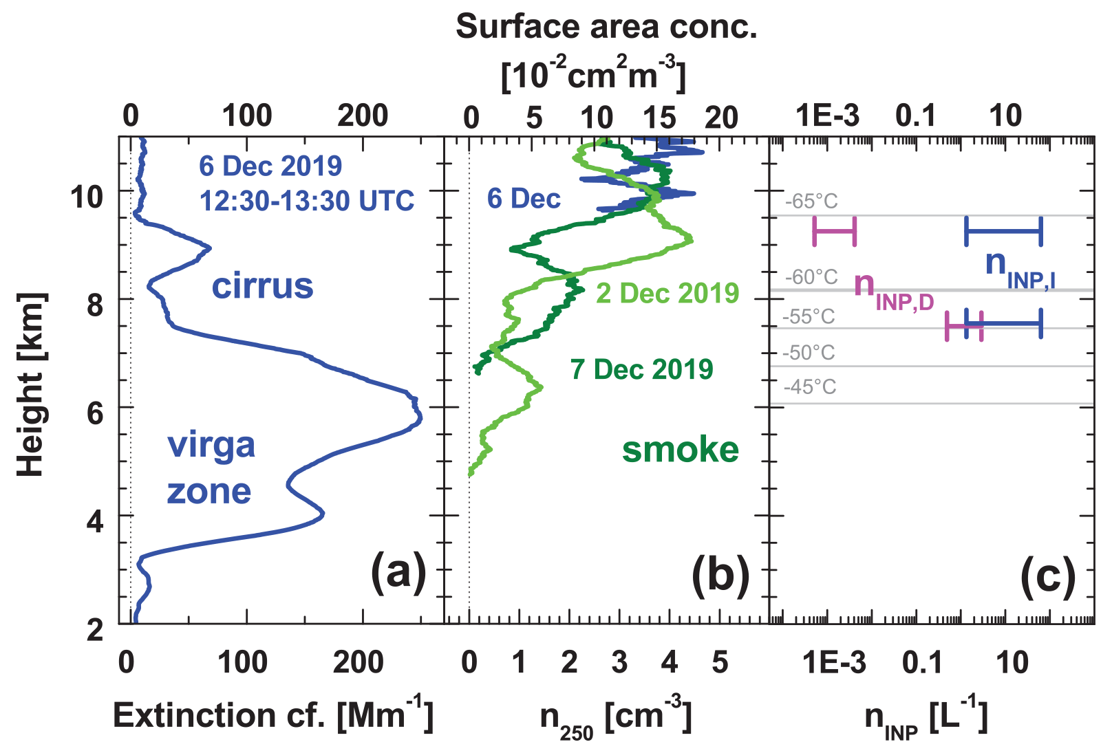
Figure 17(a) Mean cirrus extinction coefficient σ (532 nm) for the cirrus segment measured on 6 December 2019, 12:30–13:30 UTC. (b) Estimated smoke particle number concentration n250 for large particles with diameters >500 nm and particle surface area concentration s retrieved from the lidar observations for the cloud-free days of 2 and 7 December (green, olive) and for 6 December (in blue, above the cirrus), and (c) estimated ranges of INP number concentrations nINP,I (for immersion freezing, blue) and nINP,D (for deposition nucleation, in pink). Δaw ranged from 0.225 to 0.25; correspondingly the ice supersaturation Si ranged from 1.37–1.41 (at 7.5 km height, −55.4 ∘C) and from 1.4 to 1.44 (at 9.25 km height, −64 ∘C). The particle surface area concentration was set to s=0.05 cm2 m−3 and the updraft time period to Δt=600 s in the smoke INP computations with Eqs. (1) and (2).
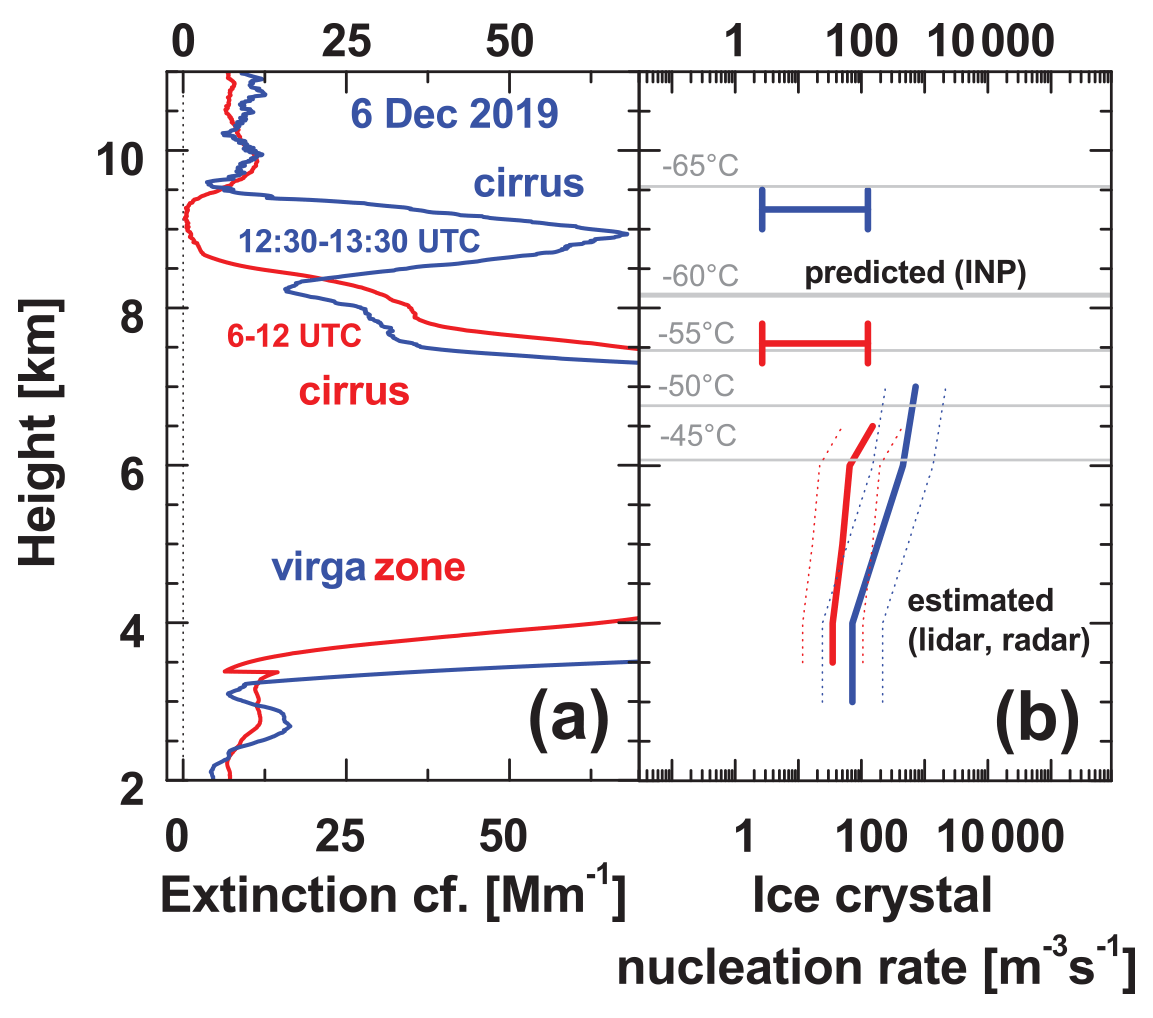
Figure 18(a) Temporally averaged (mean) cirrus extinction coefficient σ (532 nm) for two cirrus periods from 06:00–12:00 UTC (red) and from 12:30–13:30 UTC (blue) on 6 December 2019. (b) Predicted ice crystal nucleation rate, i.e., nINP,I for Δt=1 s in Eq. (1) (horizontal bars), and estimated ice crystal nucleation rates (vertical lines) obtained from the lidar–radar observations in the virga zone for the 06:00–12:00 UTC (red) and 12:30–13:30 UTC (blue) time periods. The thin dotted lines show the uncertainty (factor of 3) in the lidar–radar retrievals.
The data analysis with respect to ice nucleation on smoke particles is explained in Figs. 17 and 18. We applied the water-activity-based immersion freezing model (ABIFM) that allows predicting of immersion freezing under cirrus conditions (Knopf and Alpert, 2013). The following equation is used to compute the number concentration of smoke INP for the immersion freezing mode (Knopf and Alpert, 2013):
with the surface area concentration s of the smoke particles in cm2 m−3, the ice crystal nucleation rate coefficient Jhet,I (in cm−2 s−1), and the time period Δt (in seconds) for which constant or almost constant ice supersaturation conditions are assumed. This can be the time period of a short updraft event (of a few minutes, 120–300 s) or the duration of the lifting period of a gravity wave of typically 600±200 s (Kalesse and Kollias, 2013). The ice nucleation rate coefficient Jhet,I is a function of the organic material in the (liquid) shell of the smoke particle and the water-activity criterion Δaw (Koop et al., 2000). Δaw, shown in Fig. 15c, describes the difference between the ice melting conditions and the observed freezing conditions as a function of temperature and humidity as measured with the radiosonde. In the computation, Δaw is obtained from the difference between the actually occurring RHw (over water) and the ice-saturation-related RHw,sat value for the observed (actually occurring) temperature (with RHw and RHw,sat in decimal numbers). Δaw must reach values of 0.2–0.27 or even 0.29 to initiate significant ice nucleation (see vertical lines in Fig. 15c). Homogeneous ice nucleation is characterized by Δaw≈0.313 (Knopf and Rigg, 2011). As can be seen, Δaw takes values of 0.1–0.2 according to the radiosonde observations. Δaw values of 0.22–0.29 are only reached here during vertical motion of air parcels.
For a demonstration of our method, we chose to apply the ABIFM for leonardite (a standard humic-acid surrogate material) to represent the amorphous organic coating of smoke particles. An alternative natural organic substance would be Pahokee peat (Knopf and Alpert, 2013). Leonardite, an oxidation product of lignite, is a humic-acid-containing soft waxy particle (mineraloid), black or brown in color, and soluble in alkaline solutions. Both substances (leonardite or Pahokee peat) served as surrogates for HULISs in extended immersion freezing laboratory studies.
Similarly, we calculate the INP number concentration for the deposition ice nucleation (DIN) mode (Wang and Knopf, 2011):
The ice nucleation rate coefficient Jhet,D requires information on temperature T and ice supersaturation Si, also shown in Fig. 15c, and parameters describing the ice nucleation potential of the organic material. Also in the case of DIN, laboratory results for leonardite were used (Wang and Knopf, 2011). A more detailed description of smoke INP computation may be found in Ansmann et al. (2021).
Figure 17 provides an overview of all retrieval products necessary to evaluate the potential of smoke particles to serve as INP. From the aerosol lidar observations (backscattering in cloud-free conditions) we obtain estimates for the particle surface area concentration s (Ansmann et al., 2021). We show the aerosol conditions at different days in Fig. 17b (before, during, and after the cirrus event) and used the respective lidar backscatter profiles to estimate the surface area concentration of the smoke particles. It can be concluded that the smoke surface area concentration was in the range of 0.05–0.15 cm2 m−3 during the formation of ice crystals at 7–7.5 km and at 9.0–9.5 km in the case of the cirrus layer in Fig. 17a. In Fig. 17b, the estimated number concentration of large smoke particles n250 (with radius ≥250 nm, lower axis) is also shown. n250 may be interpreted as the overall reservoir of potential smoke INPs. It is assumed that larger particles provide better ice nucleation conditions than smaller particles. The uncertainty in the aerosol estimates is about 20 %–25 % (Table 1).
Figure 17c shows the results of the INPC calculations with Eqs. (1) and (2). The range of immersion freezing INPC (i.e., the length of the respective two horizontal bars in Fig. 17c) is obtained by computing nINP,I with Eq. (1) for Δaw of 0.225 and 0.25. The particle surface area concentration of 0.05 cm2 m−3 is used in these computations and Δt is set to 600 s. In the case of the deposition nucleation INPC, the shown INPC range (length of each bar) is obtained by computing nINP,D with Eq. (2) for the corresponding ice supersaturation values Si from 1.37–1.41 (7–7.5 km height, −55.4 ∘C) and from 1.41–1.44 (9–9.5 km height, −64 ∘C). As can be seen, nINP,I ranged from 1–63 L−1 at both heights (for the same Δaw range), and for nINP,D, we obtained values from 0.4–3 L−1 at 7–7.5 km height and <0.01 L−1 at 9–9.5 km height. The uncertainty in these estimates is unspecified. This is the first attempt to estimate aged smoke INP under realistic atmospheric conditions with parameterizations developed under laboratory conditions.
In the final step, we compare the immersion freezing INPC values in Fig. 17c, which can also be interpreted as predicted ice crystal numbers, with estimated ice crystal numbers derived from combined lidar–radar observations. The lidar–radar ICNC retrieval was already explained in Sect. 3.3. In this MOSAiC cirrus closure study, we used the strong and most accurate observations of radar reflectivity in the lower part of the virga zones from 4–7 km height. Since Eqs. (1) and (2) primarily deliver ice crystal nucleation rates (for Δt=1 s), we compare nucleation rate values in Fig. 18b. As pointed out by Bühl et al. (2019), the ice crystal downward flux (in m−2 s−1) is the most direct result of lidar–radar retrievals because besides radar reflectivity, the falling velocity is also measured with the Doppler radar. And this crystal flux rate can be interpreted as the ice nucleation rate as long as crystal–crystal collision and aggregation processes do not change the ice crystal number concentration too much, on the way from the cloud top region (ice nucleation region) to the lower part of the virga zones. However, this assumption may be strongly violated as Mitchell et al. (2018) concluded from CALIPSO lidar observations. They found that the ice crystal number concentration in the virga may be lower by a factor of 3–5 compared to the ICNC values at cloud top. On the other hand, the crystal nucleation rates we discuss below were quite low so that the aggregation effect may have been small (of the order of a factor of 2 or less for this Arctic ice cloud system). Other ICNC-influencing effects, e.g., secondary ice formation can be ignored in the case of cold cirrus clouds (Field et al., 2006; Korolev and Leisner, 2020). The low lidar–radar-estimated ICNC values of 40–70 m−3 or 0.04–0.07 L−1 (mean values for the virga between 4–6 km height for the period from 06:00–12:00 UTC, not shown here) and about 150 m−3 or 0.15 L−1 higher up (based on less accurate radar reflectivity measured at 6–7 km height) corroborate the idea that the aggregation-related uncertainty in our lidar–radar estimate of the ice crystal nucleation rate at cloud top may have been low. For the time period from 12:00–14:00 UTC, the lidar–radar retrieval yielded ICNC values of 80–500 m−3 or 0.08–0.5 L−1in the virga layer from 4–6 km height and about 800 m−3 at 7 km height.
In our cirrus closure experiment, the goal is now to check how well the two numbers of the predicted and the estimated ice crystal nucleation rates are in agreement. The question behind this is as follows: can the smoke INP parameterizations reproduce these values given by the lidar–radar observations so that we can conclude that smoke particles most likely controlled the evolution of the cirrus deck and the virga and respective ice crystal microphysical properties? In the case of a successful closure experiment, we may even conclude that the applied INP parameterization is appropriate to be used in models to predict the smoke impact on cirrus formation.
As shown in Fig. 18b, the lidar–radar retrieval yielded ice crystal nucleation rates of 10–200 m−3 s−1 and 50–1000 m−3 s−1 (derived from the crystal flux observations between 4 and 6 km height) for the cirrus period from 06:00–12:00 UTC and 12:00–14:00 UTC, respectively. The prediction (based on INP retrieval with Eq. (1) for Δt=1 s) reveals 1–100 m−3 s−1 at cirrus top layer level. This can be regarded as a reasonable agreement keeping in mind that the particle surface area concentrations may have been underestimated, stronger updrafts may have occurred causing significantly higher Δaw values than 0.25 (at a value of Δaw=0.27 we obtain an order of magnitude higher nucleation rates), or leonardite is not representing well the organic material in the liquid shell of the smoke particles. With Pahokee peat parameters we obtain a factor of 3 higher ice crystal nucleation rates (or INPC values).
To sum up, heterogeneous ice nucleation is a complex process, especially in the case of organic aerosol particles. However, the successful closure, indicated by a reasonable match between the predicted ice crystal nucleation rate (from the nINP,I computation) and the estimated ice crystal nucleation rate (from lidar–radar observations) shows that the wildfire smoke was probably able to trigger cirrus formation (before the ice supersaturation onset for homogeneous freezing was reached) and to control the further evolution of the ice cloud system. The facts that (a) the radiosondes showed permanent ice supersaturation conditions in the virga over the day (a sign of low ICNC values in the virga) and (b) that the lidar–radar retrievals pointed to rather low ice crystal nucleation rates are independent indications that the heterogeneous ice formation was most probably responsible for the observed cirrus evolution or at least controlled the microphysical properties on 6 December 2019. It is clear that many more closure studies are needed to obtain a statistically trustworthy view on smoke and the role in cirrus ice nucleation. The respective extended data analysis will be part of our MOSAiC data analysis.
The goal of this introductory article was to present some highlights and key findings of the MOSAiC winter half year and also to provide an overview of the capabilities of modern lidar methods to contribute to Arctic research in the field of aerosols, clouds, and aerosol–cloud interaction. Continuous observations were performed mostly at latitudes >85∘ N during the MOSAiC months from September 2019 to May 2020.
The highlight of our observations was the detection of the long-lasting UTLS wildfire smoke layer which was present over the North Pole region for more than 7 months. A detailed analysis of the smoke properties and the potential impact on the record-breaking ozone reduction can be found in Ohneiser et al. (2021). Besides the smoke, we presented 2 d with typical Arctic haze layering features and properties. The results agree well with foregoing studies performed in the framework of POLARCAT-IPY and ARCTAS.
Our research focus is on aerosol–cloud interaction, especially on ice nucleation in mixed-phase clouds and cirrus in the middle and upper troposphere. We developed new techniques, data analysis concepts, and closure experiments and applied them for the first time to Arctic cloud studies. These successful closure experiments (demonstrated in two case studies) corroborate that aerosol particles are able to control cloud evolution and cloud microphysical properties.
As a future work, we will analyze the 1-year MOSAiC data set to characterize the annual cycle of aerosol and cloud conditions and will contrast winter with summer conditions especially regarding aerosol–cloud interaction at cirrus level. Aerosol conditions during winter and early spring are very different from the ones during the summer and early autumn season and thus the impact of aerosol particles on mixed-phase cloud and cirrus evolution should be different as well.
Such large campaigns as the MOSAiC expedition offer the unique opportunity to introduce and apply new techniques and concepts of data analysis methods and integrate them into the existing instrumentation infrastructures and routine monitoring and observational data processing. However, to better characterize the uncertainties in our estimated and retrieved aerosol and cloud products and to narrow the uncertainty ranges, field campaigns with frequent overflights of remote-sensing stations by aircraft measuring cloud-relevant aerosol properties as well as cloud microphysical properties in situ are required in the framework of validation efforts. Such comprehensive aircraft remote-sensing field campaigns are also needed to improve our knowledge on the basic features of the complex processes of aerosol–cloud interactions.
Because of the importance of the Arctic in the climate system it would be desirable to establish at least one supersite in the High Arctic for remote-sensing and in situ observations (with balloon, unmanned aerial vehicles, aircraft) of aerosol and cloud properties in the lower, middle, and upper free troposphere and the lower stratosphere. This station should perform year-round measurements to document the fast changes in the atmospheric and environmental conditions in the Arctic, to better understand the role of aerosols in cloud formation and ozone depletion processes, and also to validate established and new remote-sensing-based retrieval methods.
Polly lidar observations (level 0 data, measured signals) are in the PollyNET database (PollyNET, 2020) with quick looks at http://picasso.tropos.de (last access: 15 July 2021). All the analysis products are available at TROPOS upon request (polly@tropos.de). The AMF-1 cloud radar data are provided by the ARM MOSAiC user facility (ARM-MOSAiC, 2021). In addition, all MOSAiC consortium members have early access to the data via the MOSAiC Central Storage (MCS) system before the data become publicly released on 1 January 2023. The radiosonde data are available at https://doi.org/10.1594/PANGAEA.928656 (Maturilli et al., 2021). PANGAEA is the primary long-term archive for the MOSAiC data set. KAZR data are available via the ARM data archive (https://adc.arm.gov/discovery/, last access: 15 July 2021).
The paper was written by RE and AA with contributions (data analysis) from KO, HB, CJ, JB, HeG, MH, SD, MM, IV, and PS. The co-authors HaG, MR, JH, and DA as well as RE took care of the lidar observations aboard Polarstern during the MOSAiC year. CJ and RW implemented and tested the new dual-FOV polarization lidar channels. UW and AM were involved in the data interpretation and discussions of the observations.
The authors declare that they have no conflict of interest.
Publisher's note: Copernicus Publications remains neutral with regard to jurisdictional claims in published maps and institutional affiliations.
We are grateful to the MOSAiC teams and the Polarstern crew for their perfect logistical support. Cloud radar data were provided by the US Department of Energy's Atmospheric Radiation Measurement Program. We further thank the entire radiosonde team, especially AWI, DWD, ARM, Jürgen (Egon) Graeser, and all volunteers for their enormous efforts of producing the exemplary and uninterrupted 6-hourly data set in the full MOSAiC year.
The data were produced as part of the international Multidisciplinary drifting Observatory for the Study of the Arctic Climate (MOSAiC) with the tag MOSAiC20192020 and project ID AWI_PS122_00. This project has also received funding from the European Union's Horizon 2020 research and innovation program ACTRIS-2 Integrating Activities (H2020-INFRAIA-2014–2015, grant no. 654109). We gratefully acknowledge the funding by the Deutsche Forschungsgemeinschaft (DFG, German Research Foundation) – project no. 268020496 – TRR 172, within the Transregional Collaborative Research Center “ArctiC Amplification: Climate Relevant Atmospheric and SurfaCe Processes, and Feedback Mechanisms (AC)3”. The development of the lidar inversion algorithm used to analyze Polly data was supported by the Russian Science Foundation (project no. 16-17-10241).
This paper was edited by Geraint Vaughan and reviewed by Eleni Marinou and one anonymous referee.
Abbatt, J. P. D., Leaitch, W. R., Aliabadi, A. A., Bertram, A. K., Blanchet, J.-P., Boivin-Rioux, A., Bozem, H., Burkart, J., Chang, R. Y. W., Charette, J., Chaubey, J. P., Christensen, R. J., Cirisan, A., Collins, D. B., Croft, B., Dionne, J., Evans, G. J., Fletcher, C. G., Galí, M., Ghahremaninezhad, R., Girard, E., Gong, W., Gosselin, M., Gourdal, M., Hanna, S. J., Hayashida, H., Herber, A. B., Hesaraki, S., Hoor, P., Huang, L., Hussherr, R., Irish, V. E., Keita, S. A., Kodros, J. K., Köllner, F., Kolonjari, F., Kunkel, D., Ladino, L. A., Law, K., Levasseur, M., Libois, Q., Liggio, J., Lizotte, M., Macdonald, K. M., Mahmood, R., Martin, R. V., Mason, R. H., Miller, L. A., Moravek, A., Mortenson, E., Mungall, E. L., Murphy, J. G., Namazi, M., Norman, A.-L., O'Neill, N. T., Pierce, J. R., Russell, L. M., Schneider, J., Schulz, H., Sharma, S., Si, M., Staebler, R. M., Steiner, N. S., Thomas, J. L., von Salzen, K., Wentzell, J. J. B., Willis, M. D., Wentworth, G. R., Xu, J.-W., and Yakobi-Hancock, J. D.: Overview paper: New insights into aerosol and climate in the Arctic, Atmos. Chem. Phys., 19, 2527–2560, https://doi.org/10.5194/acp-19-2527-2019, 2019. a, b
Achtert, P. and Tesche, M.: Assessing lidar‐based classification schemes for polar stratospheric clouds based on 16 years of measurements at Esrange, Sweden, J. Geophys. Res.-Atmos., 119, 1386–1405, https://doi.org/10.1002/2013JD020355, 2014. a, b
ACTRIS: Aerosols, Clouds and Trace gases Research InfraStructure home page, avaialble at https://www.actris.eu/, last access: 20 October 2020. a
Ancellet, G., Pelon, J., Blanchard, Y., Quennehen, B., Bazureau, A., Law, K. S., and Schwarzenboeck, A.: Transport of aerosol to the Arctic: analysis of CALIOP and French aircraft data during the spring 2008 POLARCAT campaign, Atmos. Chem. Phys., 14, 8235–8254, https://doi.org/10.5194/acp-14-8235-2014, 2014. a
Andronache, C. (Ed.): Mixed-Phase Clouds, Elsevier, 1 Edn., the Netherlands, UK, USA, 2018. a
Ansmann, A., Mamouri, R.-E., Bühl, J., Seifert, P., Engelmann, R., Hofer, J., Nisantzi, A., Atkinson, J. D., Kanji, Z. A., Sierau, B., Vrekoussis, M., and Sciare, J.: Ice-nucleating particle versus ice crystal number concentration in altocumulus and cirrus layers embedded in Saharan dust:a closure study, Atmos. Chem. Phys., 19, 15087–15115, https://doi.org/10.5194/acp-19-15087-2019, 2019. a, b, c, d
Ansmann, A., Ohneiser, K., Mamouri, R.-E., Knopf, D. A., Veselovskii, I., Baars, H., Engelmann, R., Foth, A., Jimenez, C., Seifert, P., and Barja, B.: Tropospheric and stratospheric wildfire smoke profiling with lidar: mass, surface area, CCN, and INP retrieval, Atmos. Chem. Phys., 21, 9779–9807, https://doi.org/10.5194/acp-21-9779-2021, 2021. a, b, c, d
ARM: Atmospheric Radiation Measurement (ARM) mobile facility homepage, available at https://www.arm.gov/capabilities/observatories/amf, last access: 20 October 2020. a
ARM-MOSAiC: Atmospheric Radiation Measurement (ARM) user facility, 2019, updated hourly, Ka ARM Zenith Radar (KAZRCFRGE), 2019-10-11 to 2020-09-20, ARM Mobile Facility (MOS) MOSAIC (Drifting Obs – Study of Arctic Climate), AMF2 (M1), compiled by: Lindenmaier, I., Nelson, D., Isom, B., Hardin, J., Matthews, A., Wendler, T., and Castro, V., ARM Data Center, available at: https://adc.arm.gov/discovery/, last access: 15 July 2021. a, b
Avery, M. A., Ryan, R. A., Getzewich, B. J., Vaughan, M. A., Winker, D. M., Hu, Y., Garnier, A., Pelon, J., and Verhappen, C. A.: CALIOP V4 cloud thermodynamic phase assignment and the impact of near-nadir viewing angles, Atmos. Meas. Tech., 13, 4539–4563, https://doi.org/10.5194/amt-13-4539-2020, 2020. a
Baars, H., Ansmann, A., Althausen, D., Engelmann, R., Heese, B., Müller, D., Artaxo, P., Paixao, M., Pauliquevis, T., and Souza, R.: Aerosol profiling with lidar in the Amazon Basin during the wet and dry season, J. Geophys. Res., 117, D21201, https://doi.org/10.1029/2012JD018338, 2012. a
Baars, H., Kanitz, T., Engelmann, R., Althausen, D., Heese, B., Komppula, M., Preißler, J., Tesche, M., Ansmann, A., Wandinger, U., Lim, J.-H., Ahn, J. Y., Stachlewska, I. S., Amiridis, V., Marinou, E., Seifert, P., Hofer, J., Skupin, A., Schneider, F., Bohlmann, S., Foth, A., Bley, S., Pfüller, A., Giannakaki, E., Lihavainen, H., Viisanen, Y., Hooda, R. K., Pereira, S. N., Bortoli, D., Wagner, F., Mattis, I., Janicka, L., Markowicz, K. M., Achtert, P., Artaxo, P., Pauliquevis, T., Souza, R. A. F., Sharma, V. P., van Zyl, P. G., Beukes, J. P., Sun, J., Rohwer, E. G., Deng, R., Mamouri, R.-E., and Zamorano, F.: An overview of the first decade of PollyNET: an emerging network of automated Raman-polarization lidars for continuous aerosol profiling, Atmos. Chem. Phys., 16, 5111–5137, https://doi.org/10.5194/acp-16-5111-2016, 2016. a, b
Baars, H., Ansmann, A., Ohneiser, K., Haarig, M., Engelmann, R., Althausen, D., Hanssen, I., Gausa, M., Pietruczuk, A., Szkop, A., Stachlewska, I. S., Wang, D., Reichardt, J., Skupin, A., Mattis, I., Trickl, T., Vogelmann, H., Navas-Guzmán, F., Haefele, A., Acheson, K., Ruth, A. A., Tatarov, B., Müller, D., Hu, Q., Podvin, T., Goloub, P., Veselovskii, I., Pietras, C., Haeffelin, M., Fréville, P., Sicard, M., Comerón, A., Fernández García, A. J., Molero Menéndez, F., Córdoba-Jabonero, C., Guerrero-Rascado, J. L., Alados-Arboledas, L., Bortoli, D., Costa, M. J., Dionisi, D., Liberti, G. L., Wang, X., Sannino, A., Papagiannopoulos, N., Boselli, A., Mona, L., D'Amico, G., Romano, S., Perrone, M. R., Belegante, L., Nicolae, D., Grigorov, I., Gialitaki, A., Amiridis, V., Soupiona, O., Papayannis, A., Mamouri, R.-E., Nisantzi, A., Heese, B., Hofer, J., Schechner, Y. Y., Wandinger, U., and Pappalardo, G.: The unprecedented 2017–2018 stratospheric smoke event: decay phase and aerosol properties observed with the EARLINET, Atmos. Chem. Phys., 19, 15183–15198, https://doi.org/10.5194/acp-19-15183-2019, 2019. a, b, c, d, e, f
Baars, H., Herzog, A., Heese, B., Ohneiser, K., Hanbuch, K., Hofer, J., Yin, Z., Engelmann, R., and Wandinger, U.: Validation of Aeolus wind products above the Atlantic Ocean, Atmos. Meas. Tech., 13, 6007–6024, https://doi.org/10.5194/amt-13-6007-2020, 2020. a
Bailey, M., and Hallett, J.: Ice Crystal Linear Growth Rates from −20∘ to −70 ∘C: Confirmation from Wave Cloud Studies, J. Atmos. Sci., 69, 390–402, https://doi.org/10.1175/JAS-D-11-035.1, 2012. a
Barahona, D., Molod, A., and Kalesse, H.: Direct estimation of the global distribution of vertical velocity within cirrus clouds, Sci. Rep.-UK, 7, 6840, https://doi.org/10.1038/s41598-017-07038-6, 2017. a
Berkemeier, T., Shiraiwa, M., Pöschl, U., and Koop, T.: Competition between water uptake and ice nucleation by glassy organic aerosol particles, Atmos. Chem. Phys., 14, 12513–12531, https://doi.org/10.5194/acp-14-12513-2014, 2014. a
Boers, R., de Laat, A. T., Stein Zweers, D. C., and Dirksen, R. J.: Lifting potential of solar-heated aerosol layers, Geophys. Res. Lett., 37, L24802, https://doi.org/10.1029/2010GL045171, 2010. a
Bohlmann, S., Baars, H., Radenz, M., Engelmann, R., and Macke, A.: Ship-borne aerosol profiling with lidar over the Atlantic Ocean: from pure marine conditions to complex dust–smoke mixtures, Atmos. Chem. Phys., 18, 9661–9679, https://doi.org/10.5194/acp-18-9661-2018, 2018. a
Bühl, J., Seifert, P., Myagkov, A., and Ansmann, A.: Measuring ice- and liquid-water properties in mixed-phase cloud layers at the Leipzig Cloudnet station, Atmos. Chem. Phys., 16, 10609–10620, https://doi.org/10.5194/acp-16-10609-2016, 2016. a
Bühl, J., Seifert, P., Radenz, M., Baars, H., and Ansmann, A.: Ice crystal number concentration from lidar, cloud radar and radar wind profiler measurements, Atmos. Meas. Tech., 12, 6601–6617, https://doi.org/10.5194/amt-12-6601-2019, 2019. a, b, c, d
Burton, S. P., Hair, J. W., Kahnert, M., Ferrare, R. A., Hostetler, C. A., Cook, A. L., Harper, D. B., Berkoff, T. A., Seaman, S. T., Collins, J. E., Fenn, M. A., and Rogers, R. R.: Observations of the spectral dependence of linear particle depolarization ratio of aerosols using NASA Langley airborne High Spectral Resolution Lidar, Atmos. Chem. Phys., 15, 13453–13473, https://doi.org/10.5194/acp-15-13453-2015, 2015. a
CALIPSO: Cloud–Aerosol Lidar and Infrared Pathfinder Satellite Observation Lidar Level 2 data, height-time displays of attenuated backscatter, available at: https://www-calipso.larc.nasa.gov/products/lidar/browse_images/std_v4_index.php, last access: 20 October 2020a. a
CALIPSO: Cloud–Aerosol Lidar and Infrared Pathfinder Satellite Observation Lidar Level 2 data, particle backscatter profiles, available at: https://search.earthdata.nasa.gov/search?fp=CALIPSO&fi=CALIOP, last access: 20 October 2020b. a
Cazenave, Q., Ceccaldi, M., Delanoë, J., Pelon, J., Groß, S., and Heymsfield, A.: Evolution of DARDAR-CLOUD ice cloud retrievals: new parameters and impacts on the retrieved microphysical properties, Atmos. Meas. Tech., 12, 2819–2835, https://doi.org/10.5194/amt-12-2819-2019, 2019. a
China, S., Scarnato, B., Owen, R. C., Zhang, B., Ampadu, M. T., Kumar, S., Dzepina, K., Dziobak, M. P., Fialho, P., Perlinger, J. A., Hueber, J., Helmig, D., Mazzoleni, L. R., and Mazzoleni, C.: Morphology and mixing state of aged soot particles at a remote marine free troposphere site: Implications for optical properties, Geophys. Res. Lett., 42, 1243–1250, https://doi.org/10.1002/2014GL062404, 2015. a
Creamean, J. M., Cross, J. N., Pickart, R., McRaven, L., Lin, P., Pacini, A., Hanlon, R., Schmale, D. G., Ceniceros, J., Aydell, T., Colombi, N., Bolger, E., and DeMott, P. J.: Ice nucleating particles carried from below a phytoplankton bloom to the Arctic atmosphere, Geophys. Res. Lett., 46, 8572–8581, https://doi.org/10.1029/2019GL083039, 2019. a
Dahlkötter, F., Gysel, M., Sauer, D., Minikin, A., Baumann, R., Seifert, P., Ansmann, A., Fromm, M., Voigt, C., and Weinzierl, B.: The Pagami Creek smoke plume after long-range transport to the upper troposphere over Europe – aerosol properties and black carbon mixing state, Atmos. Chem. Phys., 14, 6111–6137, https://doi.org/10.5194/acp-14-6111-2014, 2014. a, b, c
Dai, G., Althausen, D., Hofer, J., Engelmann, R., Seifert, P., Bühl, J., Mamouri, R.-E., Wu, S., and Ansmann, A.: Calibration of Raman lidar water vapor profiles by means of AERONET photometer observations and GDAS meteorological data, Atmos. Meas. Tech., 11, 2735–2748, https://doi.org/10.5194/amt-11-2735-2018, 2018. a, b, c
de Laat, A. T. J., Stein Zweers, D. C., Boers, R., and Tuinder, O. N. E.: A solar escalator: Observational evidence of the self-lifting of smoke and aerosols by absorption of solar radiation in the February 2009 Australian Black Saturday plume, J. Geophys. Res., 117, D04204, https://doi.org/10.1029/2011JD017016, 2012.
DeLand, M. T., Bhartia, P. K., Kramarova, N., and Chen, Z.: OMPS LP observations of PSC variability during the NH 2019-2020 season, Geophys. Res. Lett., 47, e2020GL090216, https://doi.org/10.1029/2020GL090216, 2020. a, b
DeMott, P. J., Prenni, A. J., Liu, X., Kreidenweis, S. M., Petters, M. D., Twohy, C. H., Richardson, M. S., Eidhammer, T., and Rogers, D. C.: Predicting global atmospheric ice nuclei distributions and their impacts on climate, P. Natl. Acad. Sci. USA, 107, 11217–11222, https://doi.org/10.1073/pnas.0910818107, 2010. a
DeMott, P. J., Prenni, A. J., McMeeking, G. R., Sullivan, R. C., Petters, M. D., Tobo, Y., Niemand, M., Möhler, O., Snider, J. R., Wang, Z., and Kreidenweis, S. M.: Integrating laboratory and field data to quantify the immersion freezing ice nucleation activity of mineral dust particles, Atmos. Chem. Phys., 15, 393–409, https://doi.org/10.5194/acp-15-393-2015, 2015. a, b
Devasthale, A., Tjernström, M., Karlsson, K.-G., Thomas, M. A., Jones, C., Sedlar, J., and Omar, A. H.: The vertical distribution of thin features over the Arctic analysed from CALIPSO observations, Tellus B, 63, 77–85, https://doi.org/10.1111/j.1600-0889.2010.00516.x, 2011a. a
Devasthale, A., Tjernström, M., and Omar, A. H.: The vertical distribution of thin features over the Arctic analysed from CALIPSO observations – Part II: Aerosols, Tellus B, 63, 86–95, https://doi.org/10.1111/j.1600-0889.2010.00517.x, 2011b. a
de Villiers, R. A., Ancellet, G., Pelon, J., Quennehen, B., Schwarzenboeck, A., Gayet, J. F., and Law, K. S.: Airborne measurements of aerosol optical properties related to early spring transport of mid-latitude sources into the Arctic, Atmos. Chem. Phys., 10, 5011–5030, https://doi.org/10.5194/acp-10-5011-2010, 2010. a
Di Biagio, C., Pelon, J., Ancellet, G., Bazureau, A., and Mariage, V.: Sources, load, vertical distribution, and fate of wintertime aerosols north of Svalbard from combined V4 CALIOP data, ground‐based IAOOS lidar observations and trajectory analysis, J. Geophys. Res.-Atmos., 123, 1363–1383, https://doi.org/10.1002/2017JD027530, 2018. a, b, c, d, e, f
Di Pierro, M., Jaeglé, L., Eloranta, E. W., and Sharma, S.: Spatial and seasonal distribution of Arctic aerosols observed by the CALIOP satellite instrument (2006–2012), Atmos. Chem. Phys., 13, 7075–7095, https://doi.org/10.5194/acp-13-7075-2013, 2013. a, b
Düsing, S., Wehner, B., Seifert, P., Ansmann, A., Baars, H., Ditas, F., Henning, S., Ma, N., Poulain, L., Siebert, H., Wiedensohler, A., and Macke, A.: Helicopter-borne observations of the continental background aerosol in combination with remote sensing and ground-based measurements, Atmos. Chem. Phys., 18, 1263–1290, https://doi.org/10.5194/acp-18-1263-2018, 2018. a
Eirund, G. K., Possner, A., and Lohmann, U.: Response of Arctic mixed-phase clouds to aerosol perturbations under different surface forcings, Atmos. Chem. Phys., 19, 9847–9864, https://doi.org/10.5194/acp-19-9847-2019, 2019. a
Eloranta, E.: High Spectral Resolution Lidar, in: LIDAR – Range–resolved optical remote sensing of the atmosphere, edited by: Weitkamp, C., Springer, New York, ISBN 0-387-40075-3, 143–163, 2005. a
Engelmann, R., Kanitz, T., Baars, H., Heese, B., Althausen, D., Skupin, A., Wandinger, U., Komppula, M., Stachlewska, I. S., Amiridis, V., Marinou, E., Mattis, I., Linné, H., and Ansmann, A.: The automated multiwavelength Raman polarization and water-vapor lidar PollyXT: the neXT generation, Atmos. Meas. Tech., 9, 1767–1784, https://doi.org/10.5194/amt-9-1767-2016, 2016. a, b, c, d
Fetterer, F., Knowles, K., Meier, W. N., Savoie, M., and Windnagel, A. K.: Sea Ice Index, Version 3, 2017, Monthly Sea Ice Extent, Boulder, Colorado USA, NSIDC: National Snow and Ice Data Center, https://doi.org/10.7265/N5K072F8, last access: 15 July 2020. a
Fiebig, M., Stohl, A., Wendisch, M., Eckhardt, S., and Petzold, A.: Dependence of solar radiative forcing of forest fire aerosol on ageing and state of mixture, Atmos. Chem. Phys., 3, 881–891, https://doi.org/10.5194/acp-3-881-2003, 2003. a, b
Field, P. R., Heymsfield, A. J., and Bansemer, A.: A Test of Ice Self-Collection Kernels Using Aircraft Data, J. Atmos. Sci., 63, 651–666, https://doi.org/10.1175/JAS3653.1, 2006. a
Fromm, M., Shettle, E. P., Fricke, K. H., Ritter, C., Trickl, T., Giehl, H., Gerding, M., Barnes, J. E., O'Neill, M., Massie, S. T., Blum, U., McDermid, I. S., Leblanc, T., and Deshler, T.: Stratospheric impact of the Chisholm pyrocumulonimbus eruption: 2. Vertical profile perspective, J. Geophys. Res., 113, D08203, https://doi.org/10.1029/2007JD009147, 2008. a
Fromm, M., Lindsey, D. T., Servranckx, R., Yue, G., Trickl, T., Sica, R., Doucet, P., and Godin-Beekmann, S. E.: The untold story of pyrocumulonimbus, B. Am. Meteorol. Soc., 91, 1193–1209, https://doi.org/10.1175/2010bams3004.1, 2010. a
Georgoulias, A. K., Marinou, E., Tsekeri, A., Proestakis, E., Akritidis, D., Alexandri, G., Zanis, P., Balis, D., Marenco, F., Tesche, M., and Amiridis, V.: A first case study of CCN concentrations from spaceborne lidar observations, Remote Sens., 12, 1557, https://doi.org/10.3390/rs12101557, 2020. a
GMAO: Tropopause definition (page 52), Global Modeling and Assimilation Office, Goddard Space Flight Center, Greenbelt, Maryland, available at: https://gmao.gsfc.nasa.gov/GMAO_products/documents/GEOS-5.2.0_File_Specification.pdf, last access: 19 February 2021. a
Grenier, P., Blanchet, J. P., and Munoz-Alpizar, R.: Study of polar thin ice clouds and aerosols seen by CloudSat and CALIPSO during mid-winter 2007, J. Geophys. Res., 114, D09201, https://doi.org/10.1029/2008JD010927, 2009. a
Griesche, H. J., Seifert, P., Ansmann, A., Baars, H., Barrientos Velasco, C., Bühl, J., Engelmann, R., Radenz, M., Zhenping, Y., and Macke, A.: Application of the shipborne remote sensing supersite OCEANET for profiling of Arctic aerosols and clouds during Polarstern cruise PS106, Atmos. Meas. Tech., 13, 5335–5358, https://doi.org/10.5194/amt-13-5335-2020, 2020. a
Griesche, H. J., Ohneiser, K., Seifert, P., Radenz, M., Engelmann, R., and Ansmann, A.: Contrasting ice formation in Arctic clouds: surface-coupled vs. surface-decoupled clouds, Atmos. Chem. Phys., 21, 10357–10374, https://doi.org/10.5194/acp-21-10357-2021, 2021. a
Groß, S., Gasteiger, J., Freudenthaler, V., Müller, T., Sauer, D., Toledano, C., and Ansmann, A.: Saharan dust contribution to the Caribbean summertime boundary layer – a lidar study during SALTRACE, Atmos. Chem. Phys., 16, 11535–11546, https://doi.org/10.5194/acp-16-11535-2016, 2016. a
Haarig, M., Ansmann, A., Baars, H., Jimenez, C., Veselovskii, I., Engelmann, R., and Althausen, D.: Depolarization and lidar ratios at 355, 532, and 1064 nm and microphysical properties of aged tropospheric and stratospheric Canadian wildfire smoke, Atmos. Chem. Phys., 18, 11847–11861, https://doi.org/10.5194/acp-18-11847-2018, 2018. a, b
Haarig, M., Walser, A., Ansmann, A., Dollner, M., Althausen, D., Sauer, D., Farrell, D., and Weinzierl, B.: Profiles of cloud condensation nuclei, dust mass concentration, and ice-nucleating-particle-relevant aerosol properties in the Saharan Air Layer over Barbados from polarization lidar and airborne in situ measurements, Atmos. Chem. Phys., 19, 13773–13788, https://doi.org/10.5194/acp-19-13773-2019, 2019. a, b
Hartmann, M., Adachi, K., Eppers, O., Haas, C., Herber, A., Holzinger, R., Hünerbein, A., Jäkel, E., Jentzsch, C., van Pinxteren, M., Wex, H., Willmes, S., and Stratmann, F.: Wintertime airborne measurements of ice nucleating particles in the High Arctic: a hint to a marine, biogenic source for icenucleating particles, Geophys. Res. Lett., 47, e2020GL087770, https://doi.org/10.1029/2020GL087770, 2020. a
Hofer, J., Althausen, D., Abdullaev, S. F., Makhmudov, A. N., Nazarov, B. I., Schettler, G., Engelmann, R., Baars, H., Fomba, K. W., Müller, K., Heinold, B., Kandler, K., and Ansmann, A.: Long-term profiling of mineral dust and pollution aerosol with multiwavelength polarization Raman lidar at the Central Asian site of Dushanbe, Tajikistan: case studies, Atmos. Chem. Phys., 17, 14559–14577, https://doi.org/10.5194/acp-17-14559-2017, 2017. a, b
Hofer, J., Ansmann, A., Althausen, D., Engelmann, R., Baars, H., Abdullaev, S. F., and Makhmudov, A. N.: Long-term profiling of aerosol light extinction, particle mass, cloud condensation nuclei, and ice-nucleating particle concentration over Dushanbe, Tajikistan, in Central Asia, Atmos. Chem. Phys., 20, 4695–4711, https://doi.org/10.5194/acp-20-4695-2020, 2020. a
HYSPLIT: HYbrid Single-Particle Lagrangian Integrated Trajectory model, backward trajectory calculation tool, available at: http://ready.arl.noaa.gov/HYSPLIT_traj.php, last access: 20 October 2020. a
Inness, A., Chabrillat, S., Flemming, J., Huijnen, V., Langenrock, B., Nicolas, J., Polichtchouk, I., and Razingeret, M.: Exceptionally low Arctic stratospheric ozone in spring 2020 as seen in the CAMS reanalysis, J. Geophys. Res.-Atmos., 125, e2020JD033563, https://doi.org/10.1029/2020JD033563, 2020. a
Jimenez, C., Ansmann, A., Engelmann, R., Donovan, D., Malinka, A., Schmidt, J., Seifert, P., and Wandinger, U.: The dual-field-of-view polarization lidar technique: a new concept in monitoring aerosol effects in liquid-water clouds – theoretical framework, Atmos. Chem. Phys., 20, 15247–15263, https://doi.org/10.5194/acp-20-15247-2020, 2020a. a, b, c, d, e
Jimenez, C., Ansmann, A., Engelmann, R., Donovan, D., Malinka, A., Seifert, P., Wiesen, R., Radenz, M., Yin, Z., Bühl, J., Schmidt, J., Barja, B., and Wandinger, U.: The dual-field-of-view polarization lidar technique: a new concept in monitoring aerosol effects in liquid-water clouds – case studies, Atmos. Chem. Phys., 20, 15265–15284, https://doi.org/10.5194/acp-20-15265-2020, 2020b. a, b, c, d, e, f
Johnson, M. S., Strawbridge, K., Knowland, K. E., Keller, C., and Travis, M.: Long-range transport of Siberian biomass burning emissions to North America during FIREX-AQ, Atmos. Environ., 252, 118241, https://doi.org/10.1016/j.atmosenv.2021.118241, 2021. a, b
Jouan, C., Girard, E., Pelon, J., Gultepe, I., Delanoë, J., and Blanchet, J. P.: Characterization of Arctic ice cloud properties observed during ISDAC, J. Geophys. Res., 117, D23207, https://doi.org/10.1029/2012JD017889, 2012. a
Jouan, C., Pelon, J., Girard, E., Ancellet, G., Blanchet, J. P., and Delanoë, J.: On the relationship between Arctic ice clouds and polluted air masses over the North Slope of Alaska in April 2008, Atmos. Chem. Phys., 14, 1205–1224, https://doi.org/10.5194/acp-14-1205-2014, 2014. a
Kalesse, H. and Kollias, P.: Climatology of high cloud dynamics using profiling ARM Doppler radar observations, J. Climate, 26, 6340–6359, https://doi.org/10.1175/JCLI-D-12-00695.1, 2013. a
Kanitz, T., Seifert, P., Ansmann, A., Engelmann, R., Althausen, D., Casiccia, C., and Rohwer, E. G.: Contrasting the impact of aerosols at northern and southern midlatitudes on heterogeneous ice formation, Geophys. Res. Lett., 38, L17802, https://doi.org/10.1029/2011GL048532, 2011. a
Kanitz, T., Ansmann, A., Engelmann, R., and Althausen, D.: North-south cross sections of the vertical aerosol distribution over the Atlantic Ocean from multiwavelength Raman/polarization lidar during Polarstern cruises, J. Geophys. Res.-Atmos., 118, 2643–2655, https://doi.org/10.1002/jgrd.50273, 2013. a
Kanji, Z. A., Ladino, L. A., Wex, H., Boose, Y., Burkert-Kohn, M., Cziczo, D. J., and Krämer, M.: Chapter 1: Overview of ice nucleating particles, Meteor Monogr., Am. Meteorol. Soc., 58, 1.1–1.33, https://doi.org/10.1175/amsmonographs-d-16-0006.1, 2017. a, b
Kanji, Z. A., Welti, A., Corbin, J. C., and Mensah, A. A.: Black carbon particles do not matter for immersion mode ice nucleation, Geophys. Res. Lett., 46, e2019GL086764, https://doi.org/10.1029/2019GL086764, 2020. a, b
Khaykin, S. M., Godin-Beekmann, S., Hauchecorne, A., Pelon, J., Ravetta, F., and Keckut, P.: Stratospheric smoke with unprecedentedly high backscatter observed by lidars above southern France, Geophys. Res. Lett., 45, 1639–1646, https://doi.org/10.1002/2017GL076763, 2018. a
Kim, M.-H., Omar, A. H., Tackett, J. L., Vaughan, M. A., Winker, D. M., Trepte, C. R., Hu, Y., Liu, Z., Poole, L. R., Pitts, M. C., Kar, J., and Magill, B. E.: The CALIPSO version 4 automated aerosol classification and lidar ratio selection algorithm, Atmos. Meas. Tech., 11, 6107–6135, https://doi.org/10.5194/amt-11-6107-2018, 2018. a
Klehr, D.: Charakterisierung der Tropopause über Ny-Alesund, Spitzbergen, Bachelor thesis, University Potsdam, available at: http://hdl.handle.net/10013/epic.43630 (last access: 20 April 2021), 2012. a
Kloss, C., Berthet, G., Sellitto, P., Ploeger, F., Taha, G., Tidiga, M., Eremenko, M., Bossolasco, A., Jégou, F., Renard, J.-B., and Legras, B.: Stratospheric aerosol layer perturbation caused by the 2019 Raikoke and Ulawun eruptions and their radiative forcing, Atmos. Chem. Phys., 21, 535–560, https://doi.org/10.5194/acp-21-535-2021, 2021. a
Knopf, D. A. and Alpert, P. A.: A water activity based modelof heterogeneous ice nucleation kinetics for freezing of waterand aqueous solution droplets, Farad. Discuss., 165, 513–534, https://doi.org/10.1039/c3fd00035d, 2013. a, b, c
Knopf, D. A. and Rigg, Y. J.: Homogeneous ice nucleation from aqueous inorganic/organic particles representative of biomass burning: Water activity, freezing temperatures, nucleation rates, J. Phys. Chem. A, 115, 762–773, https://doi.org/10.1021/jp109171g, 2011. a
Knopf, D. A., Alpert, P. A., and Wang, B.:, The role of organic aerosol in atmospheric ice nucleation: a review, ACS Earth and Space Chemistry, 2, 168–202, https://doi.org/10.1021/acsearthspacechem.7b00120, 2018. a, b, c
Knust, R.: Polar Research and Supply Vessel Polarstern operated by the Alfred-Wegener-Institute, Journal of large-scale research facilities, 3, A119, https://doi.org/10.17815/jlsrf-3-163, 2017. a
Koop, T., Luo, B. P., Tsias, A., and Peter, T.: Water activity as the determinant for homogeneous ice nucleation in aqueous solutions, Nature, 406, 611–614, https://doi.org/10.1038/35020537, 2000. a, b
Korolev, A. and Leisner, T.: Review of experimental studies of secondary ice production, Atmos. Chem. Phys., 20, 11767–11797, https://doi.org/10.5194/acp-20-11767-2020, 2020. a
Law, K. S., Stohl, A., Quinn, P. K., Brock, C. A., Burkhart, J. F., Paris, J.-D., Ancellet, G., Singh, H. B., Roiger, A., Schlager, H., Dibb, J., Jacob, D. J., Arnold, S. R., Pelon, J., and Thomas, J. L.: Arctic Air Pollution: New Insights from POLARCAT-IPY, B. Am. Meteorol. Soc., 95, 1873–1895, https://doi.org/10.1175/BAMS-D-13-00017.1, 2014. a, b
Lawrence, Z. D., Perlwitz, J., Butler, A. H., Manney, G. L., Newman, P. A., Lee, S. H., and Nash, E. R.: The Remarkably Strong Arctic Stratospheric Polar Vortex of Winter 2020: Links to Record‐Breaking Arctic Oscillation and Ozone Loss. J. Geophys. Res.-Atmos., 125, e2020JD033271, https://doi.org/10.1029/2020JD033271, 2020. a
Levin, E. J. T., McMeeking, G. R., DeMott, P. J., McCluskey, C. S., Carrico, C. M., Nakao, S., Jayarathne, T., Stone, E. A., Stockwell, C. E., Yokelson, R. J., and Kreidenweis, S. M.: Ice-nucleating particle emissions from biomass combustion and the potential importance of soot aerosol, J. Geophys. Res., 121, 5888–5903, https://doi.org/10.1002/2016JD024879, 2016. a
Loewe, K., Ekman, A. M. L., Paukert, M., Sedlar, J., Tjernström, M., and Hoose, C.: Modelling micro- and macrophysical contributors to the dissipation of an Arctic mixed-phase cloud during the Arctic Summer Cloud Ocean Study (ASCOS), Atmos. Chem. Phys., 17, 6693–6704, https://doi.org/10.5194/acp-17-6693-2017, 2017. a
Mamali, D., Marinou, E., Sciare, J., Pikridas, M., Kokkalis, P., Kottas, M., Binietoglou, I., Tsekeri, A., Keleshis, C., Engelmann, R., Baars, H., Ansmann, A., Amiridis, V., Russchenberg, H., and Biskos, G.: Vertical profiles of aerosol mass concentration derived by unmanned airborne in situ and remote sensing instruments during dust events, Atmos. Meas. Tech., 11, 2897–2910, https://doi.org/10.5194/amt-11-2897-2018, 2018. a
Mamouri, R.-E. and Ansmann, A.: Potential of polarization lidar to provide profiles of CCN- and INP-relevant aerosol parameters, Atmos. Chem. Phys., 16, 5905–5931, https://doi.org/10.5194/acp-16-5905-2016, 2016. a, b, c, d, e, f
Mamouri, R.-E. and Ansmann, A.: Potential of polarization/Raman lidar to separate fine dust, coarse dust, maritime, and anthropogenic aerosol profiles, Atmos. Meas. Tech., 10, 3403–3427, https://doi.org/10.5194/amt-10-3403-2017, 2017. a
Manney, G. L., Livesey, N. J., Santee, M. L., Froidevaux, L., Lambert, A., Lawrence, Z. D., Millán, L. F., Neu, J. L., Read, W. G., Schwartz, M. J., and Fuller, R. A.: Record‐low Arctic stratospheric ozone in 2020: MLS observations of chemical processes and comparisons with previous extreme winters. Geophys. Res. Lett., 47, e2020GL089063, https://doi.org/10.1029/2020GL089063, 2020. a
Marinou, E., Tesche, M., Nenes, A., Ansmann, A., Schrod, J., Mamali, D., Tsekeri, A., Pikridas, M., Baars, H., Engelmann, R., Voudouri, K.-A., Solomos, S., Sciare, J., Groß, S., Ewald, F., and Amiridis, V.: Retrieval of ice-nucleating particle concentrations from lidar observations and comparison with UAV in situ measurements, Atmos. Chem. Phys., 19, 11315–11342, https://doi.org/10.5194/acp-19-11315-2019, 2019. a, b, c, d
Mason, R. H., Si, M., Chou, C., Irish, V. E., Dickie, R., Elizondo, P., Wong, R., Brintnell, M., Elsasser, M., Lassar, W. M., Pierce, K. M., Leaitch, W. R., MacDonald, A. M., Platt, A., Toom-Sauntry, D., Sarda-Estève, R., Schiller, C. L., Suski, K. J., Hill, T. C. J., Abbatt, J. P. D., Huffman, J. A., DeMott, P. J., and Bertram, A. K.: Size-resolved measurements of ice-nucleating particles at six locations in North America and one in Europe, Atmos. Chem. Phys., 16, 1637–1651, https://doi.org/10.5194/acp-16-1637-2016, 2016. a
Maturilli, M., Holdridge, D. J., Dahlke, S., Graeser, J., Sommerfeld, A., Jaiser, R., Deckelmann, H., and Schulz, A.,: Initial radiosonde data from 2019-10 to 2020-09 during project MOSAiC, Alfred Wegener Institute, Helmholtz Centre for Polar and Marine Research, Bremerhaven, PANGAEA [data set], https://doi.org/10.1594/PANGAEA.928656, 2021. a, b, c
Mauritsen, T., Sedlar, J., Tjernström, M., Leck, C., Martin, M., Shupe, M., Sjogren, S., Sierau, B., Persson, P. O. G., Brooks, I. M., and Swietlicki, E.: An Arctic CCN-limited cloud-aerosol regime, Atmos. Chem. Phys., 11, 165–173, https://doi.org/10.5194/acp-11-165-2011, 2011. a, b
McCluskey, C. S., DeMott, P. J., Prenni, A. J., Levin, E. J. T., McMeeking, G. R., Sullivan, A. P., Hill, T. C. J., Nakao, S., Carrico, C. M., and Kreidenweis, S. M.: Characteristics of atmospheric ice nucleating particles associated with biomass burning in the US: Prescribed burns and wildfire, J. Geophys. Res.-Atmos., 119, 10458–10470, https://doi.org/10.1002/2014JD021980, 2014. a
McCluskey, C. S., Ovadnevaite, J., Rinaldi, M., Atkinson, J., Belosi, F., Ceburnis, D., Marullo, S., Hill, T. C. J., Lohmann, U., Kanji, Z. A., O'Dowd, C., Kreidenweis, S. M., and DeMott, P. J.: Marine and terrestrial organic ice-nucleating particles in pristine marine to continentally influenced Northeast Atlantic air masses, J. Geophys. Res.-Atmos., 123, 6196–6212, https://doi.org/10.1029/2017JD028033, 2018. a
Mitchell, D. L., Garnier, A., Pelon, J., and Erfani, E.: CALIPSO (IIR–CALIOP) retrievals of cirrus cloud ice-particle concentrations, Atmos. Chem. Phys., 18, 17325–17354, https://doi.org/10.5194/acp-18-17325-2018, 2018. a
Morrison, H., De Boer, G., Feingold, G., Harrington, J., Shupe,M. D., and Sulia, K.: Resilience of persistent Arctic mixed-phase clouds, Nat. Geosci., 5, 11–17, 2012. a
MOSAiC: MOSAiC homepage, available at: https://mosaic-expedition.org/, last access: 20 October 2020. a
Müller, D., Wandinger, U., and Ansmann, A.: Microphysical particle parameters from extinction and backscatter lidar data by inversion with regularization: Theory, Appl. Optics, 38, 2346–2357, 1999. a
Müller, D., Mattis, I., Ansmann, A., Wehner, B., Althausen, D., Wandinger, U., and Dubovik, O.: Closure study on optical and microphysical properties of a mixed urban and Arctic haze air mass observed with Raman lidar and Sun photometer, J. Geophys. Res., 109, D13206, https://doi.org/10.1029/2003JD004200, 2004. a
Müller, D., Hostetler, C. A., Ferrare, R. A., Burton, S. P., Chemyakin, E., Kolgotin, A., Hair, J. W., Cook, A. L., Harper, D. B., Rogers, R. R., Hare, R. W., Cleckner, C. S., Obland, M. D., Tomlinson, J., Berg, L. K., and Schmid, B.: Airborne Multiwavelength High Spectral Resolution Lidar (HSRL-2) observations during TCAP 2012: vertical profiles of optical and microphysical properties of a smoke/urban haze plume over the northeastern coast of the US, Atmos. Meas. Tech., 7, 3487–3496, https://doi.org/10.5194/amt-7-3487-2014, 2014. a, b
Murray, B. J., Wilson, T. W., Dobbie, S., Cui, Z., Al-Jumur, S. M. R. K., Möhler, O., Schnaiter, M., Wagner, R., Benz, S., Niemand, M., Saathoff, H., Ebert, V., Wagner, S., and Kärcher, B.: Heterogeneous nucleation of ice particles on glassy aerosols under cirrus conditions, Nat. Geosci., 3, 233–237, https://doi.org/10.1038/ngeo817, 2010. a
Noel, V. and Chepfer, H.: A global view of horizontally oriented crystals in ice clouds from Cloud-Aerosol Lidar and Infrared Pathfinder Satellite Observation (CALIPSO), J. Geophys. Res., 115, D00H23, https://doi.org/10.1029/2009JD012365, 2010. a
Noel, V. and Sassen, K.: Study of planar ice crystal orientations in ice clouds from scanning polarization lidar observations, J. Appl.Meteorol., 44, 653–664, 2005. a
Nott, G. J. and Duck, T. J.: Lidar studies of the polar troposphere. Met. Apps, 18, 383–405, https://doi.org/10.1002/met.289, 2011. a
Ohneiser, K., Ansmann, A., Baars, H., Seifert, P., Barja, B., Jimenez, C., Radenz, M., Teisseire, A., Floutsi, A., Haarig, M., Foth, A., Chudnovsky, A., Engelmann, R., Zamorano, F., Bühl, J., and Wandinger, U.: Smoke of extreme Australian bushfires observed in the stratosphere over Punta Arenas, Chile, in January 2020: optical thickness, lidar ratios, and depolarization ratios at 355 and 532 nm, Atmos. Chem. Phys., 20, 8003–8015, https://doi.org/10.5194/acp-20-8003-2020, 2020. a, b
Ohneiser, K., Ansmann, A., Engelmann, R., Ritter, C., Chudnovsky, A., Veselovskii, I., Baars, H., Gebauer, H., Griesche, H., Radenz, M., Hofer, J., Althausen, D., Dahlke, S., and Maturilli, M.: Siberian fire smoke in the High-Arctic winter stratosphere observed during MOSAiC 2019–2020, Atmos. Chem. Phys. Discuss. [preprint], https://doi.org/10.5194/acp-2021-117, in review, 2021. a, b, c, d, e, f, g, h, i, j, k, l, m, n, o, p, q, r, s, t, u, v
Pappalardo, G., Amodeo, A., Apituley, A., Comeron, A., Freudenthaler, V., Linné, H., Ansmann, A., Bösenberg, J., D'Amico, G., Mattis, I., Mona, L., Wandinger, U., Amiridis, V., Alados-Arboledas, L., Nicolae, D., and Wiegner, M.: EARLINET: towards an advanced sustainable European aerosol lidar network, Atmos. Meas. Tech., 7, 2389–2409, https://doi.org/10.5194/amt-7-2389-2014, 2014. a
Paukert, M. and Hoose, C.: Modeling immersion freezing with aerosol-dependent prognostic ice nuclei in Arctic mixed-phaseclouds, J. Geophys. Res.-Atmos., 119, 9073–9092, 2014. a
Petters, M. D., Parsons, M. T., Prenni, A. J., DeMott, P. J., Kreidenweis, S. M., Carrico, C. M., Sullivan, A. P., McMeeking, G. R., Levin, E., Wold, C. E., Collett Jr., J. L., and Moosmüller, H.: Ice nuclei emissions from biomass burning, J. Geophys. Res.-Atmos., 114, D07209, https://doi.org/10.1029/2008JD011532, 2009. a
Petzold, A., Weinzierl, B., Huntrieser, H., Stohl, A., Real, E., Cozic, J., Fiebig, M., Hendricks, J., Lauer, A., Law, K., Roiger, A., Schlager, H., and Weingartner, E.: Perturbation of the European free troposphere aerosol by North American forest fire plumes during the ICARTT-ITOP experiment in summer 2004, Atmos. Chem. Phys., 7, 5105–5127, https://doi.org/10.5194/acp-7-5105-2007, 2007. a
PollyNet: PollyNET lidar data base, available at: http://polly.tropos.de/, last access: 20 October 2020. a
Prenni, A. J., DeMott, P. J., Sullivan, A. P., Sullivan, R. C., Kreidenweis, S. M., and Rogers, D. C.: Biomass burning as a potential source for atmospheric ice nuclei: Western wildfires and prescribed burns, Geophys. Res. Lett., 39, L11805, https://doi.org/10.1029/2012GL051915, 2012. a
Quennehen, B., Schwarzenboeck, A., Matsuki, A., Burkhart, J. F., Stohl, A., Ancellet, G., and Law, K. S.: Anthropogenic and forest fire pollution aerosol transported to the Arctic: observations from the POLARCAT-France spring campaign, Atmos. Chem. Phys., 12, 6437–6454, https://doi.org/10.5194/acp-12-6437-2012, 2012. a, b
Radenz, M., Bühl, J., Seifert, P., Baars, H., Engelmann, R., Barja González, B., Mamouri, R.-E., Zamorano, F., and Ansmann, A.: Hemispheric contrasts in ice formation in stratiform mixed-phase clouds: Disentangling the role of aerosol and dynamics with ground-based remote sensing, Atmos. Chem. Phys. Discuss. [preprint], https://doi.org/10.5194/acp-2021-360, in review, 2021. a
Reid, J. S. and Hobbs, P. V.: Physical and optical properties of young smoke from individual biomass fires in Brazil, J. Geophys. Res., 103, 32013–32030, https://doi.org/10.1029/98JD00159, 1998. a
Ritter, C., Neuber, R., Schulz, A., Markowicz, K., Stachlewska, I., Lisok, J., Makuch, P., Pakszys, P., Markuszewski, P., Rozwadowska, A., Petelski, T., Zielinski, T., Becagli, S., Traversi, R., Udisti, R., and Gausa, M.: 2014 iAREA campaign on aerosol in Spitsbergen – Part 2: Optical properties from Raman-lidar and in-situ observations at Ny-Ålesund, Atmos. Environ., 141, 1–19, https://doi.org/10.1016/j.atmosenv.2016.05.053, 2016. a
Rolph, G., Stein, A., and Stunder, B.: Real-time Environmental Applications and Display sYstem: READY, Environ. Model. Softw., 95, 210–228, https://doi.org/10.1016/j.envsoft.2017.06.025, 2017. a
Sakai, T., Uchino, O., Nagai, T., Liley, B., Morino, I., and Fujimoto, T.: Long‐term variation of stratospheric aerosols observed with lidars over Tsukuba, Japan, from 1982 and Lauder, New Zealand, from 1992 to 2015, J. Geophys. Res.-Atmos., 121, 10283–10293, https://doi.org/10.1002/2016JD025132, 2016. a
Schill, G. P., DeMott, P. J., Emerson, E. W., Rauker, A. M. C., Kodros, J. K., Suski, K. J., Hill, T. C. J., Levin, E. J. T., Pierce, J. R., Farmer, D. K., and Kreidenweis, S. M.: The contribution of black carbon to global ice nucleating particle concentrations relevant to mixed-phase clouds, P. Natl. Acad. Sci. USA, 117, 22705–22711, https://doi.org/10.1073/pnas.2001674117, 2020a. a, b
Schill, G. P., Froyd, K. D., Bian, H., Kupc, A., Williamson, C., Brock, C. A., Ray, E., Hornbrook, R. S., Hills, A. J., Apel, E. C., Chin, M., Colarco, P. R., and Murphy, D. M.: Widespread biomass burning smoke throughout the remote troposphere, Nat. Geosci., 13, 422–427, https://doi.org/10.1038/s41561-020-0586-1, 2020b. a, b, c
Schrod, J., Weber, D., Drücke, J., Keleshis, C., Pikridas, M., Ebert, M., Cvetković, B., Nickovic, S., Marinou, E., Baars, H., Ansmann, A., Vrekoussis, M., Mihalopoulos, N., Sciare, J., Curtius, J., and Bingemer, H. G.: Ice nucleating particles over the Eastern Mediterranean measured by unmanned aircraft systems, Atmos. Chem. Phys., 17, 4817–4835, https://doi.org/10.5194/acp-17-4817-2017, 2017. a
Stein, A. F., Draxler, R. R, Rolph, G. D., Stunder, B. J. B., Cohen, M. D., and Ngan, F.: NOAA's HYSPLIT atmospheric transport and dispersion modeling system, B. Am. Meteorol. Soc., 96, 2059–2077, https://doi.org/10.1175/BAMS-D-14-00110.1, 2015. a
Stohl, A.: Characteristics of atmospheric transport into the Arctic troposphere, J. Geophys. Res., 111, D11306, https://doi.org/10.1029/2005JD006888, 2006. a
Twohy, C. H., DeMott, P. J., Pratt, K. A., Subramanian, R., Kok, G. L., Murphy, S. M., Lersch, T., Heymsfield, A. J., Wang, Z., Prather, K. A., and Seinfeld, J. H.: Relationships of biomass‐burning aerosols to ice in orographic wave clouds, J. Atmos. Sci., 67, 2437–2450, https://doi.org/10.1175/2010JAS3310.1, 2010. a
Vaughan, G., Wareing, D., and Ricketts, H.: Measurement Report: Lidar measurements of stratospheric aerosol following the 2019 Raikoke and Ulawun volcanic eruptions, Atmos. Chem. Phys., 21, 5597–5604, https://doi.org/10.5194/acp-21-5597-2021, 2021. a
Verlinde, J., Harrington, J. Y., McFarquhar, G. M., Yannuzzi, V. T., Avramov, A., Greenberg, S., Johnson, N., Zhang, G., Poellot, M. R., Mather, J. H., Turner, D. D., Eloranta, E. W., Zak, B. D., Prenni, A. J., Daniel, J. S., Kok, G. L., Tobin, D. C., Holz, R., Sassen, K., Spangenberg, D., Minnis, P., Tooman, T. P., Ivey, M. D., Richardson, S. J., Bahrmann, C. P., Shupe, M., DeMott, P. J., Heymsfield, A. J., and Schofield, R.: The mixed-phase Arctic cloud experiment, B. Am. Meteorol. Soc., 88, 205–221, 2007. a
Veselovskii I., Kolgotin, A., Griaznov, V., Müller, D., Wandinger, U., and Whiteman, D.: Inversion with regularization for the retrieval of tropospheric aerosol parameters from multi-wavelength lidar sounding, Appl. Optics, 41, 3685–3699, https://doi.org/10.1364/AO.41.003685, 2002. a, b, c, d
Veselovskii, I., Dubovik, O., Kolgotin, A., Korenskiy, M., Whiteman, D. N., Allakhverdiev, K., and Huseyinoglu, F.: Linear estimation of particle bulk parameters from multi-wavelength lidar measurements, Atmos. Meas. Tech., 5, 1135–1145, https://doi.org/10.5194/amt-5-1135-2012, 2012. a
Vihtakari, M.: ggOceanMaps: Plot data on oceanographic maps using “ggplot2”, available at: https://github.com/MikkoVihtakari/ggOceanMaps, last access: 15 November 2020. a
Wandinger, U., Müller, D., Böckmann, C., Althausen, D., Matthias, V., Bösenberg, J., Weiß, V., Fiebig, M., Wendisch, M., Stohl, A., and Ansmann, A.: Optical and microphysical characterization of biomass-burning and industrial-pollution aerosols from multiwavelength lidar and aircraft measurements, J. Geophys. Res.-Atmos., 107, 7–20, https://doi.org/10.1029/2000JD000202, 2002. a
Wang, B. and Knopf, D. A.: Heterogeneous ice nucleation on particles composed of humic‐like substances impacted by O3, J. Geophys. Res., 116, D03205, https://doi.org/10.1029/2010JD014964, 2011. a, b
Wang, Q., Jacob, D. J., Fisher, J. A., Mao, J., Leibensperger, E. M., Carouge, C. C., Le Sager, P., Kondo, Y., Jimenez, J. L., Cubison, M. J., and Doherty, S. J.: Sources of carbonaceous aerosols and deposited black carbon in the Arctic in winter-spring: implications for radiative forcing, Atmos. Chem. Phys., 11, 12453–12473, https://doi.org/10.5194/acp-11-12453-2011, 2011. a, b, c
Wendisch, M., Macke, A., Ehrlich, A., Lüpkes, C., Mech, M.,Chechin, D., Dethloff, K., Velasco, C. B., Bozem, H., Brückner, M., Clemen, H.-C., Crewell, S., Donth, T., Dupuy, R., Ebell, K., Egerer, U., Engelmann, R., Engler, C., Eppers, O., Gehrmann,M., Gong, X., Gottschalk, M., Gourbeyre, C., Griesche, H., Hartmann, J., Hartmann, M., Heinold, B., Herber, A., Herrmann, H.,Heygster, G., Hoor, P., Jafariserajehlou, S., Jäkel, E., Järvinen, E., Jourdan, O., Kästner, U., Kecorius, S., Knudsen, E. M., Köllner, F., Kretzschmar, J., Lelli, L., Leroy, D., Maturilli, M., Mei, L., Mertes, S., Mioche, G., Neuber, R., Nicolaus, M., Nomokonova, T., Notholt, J., Palm, M., van Pinxteren, M., Quaas, J., Richter, P., Ruiz-Donoso, E., Schäfer, M., Schmieder, K., Schnaiter, M., Schneider, J., Schwarzenböck, A., Seifert, P., Shupe, M. D., Siebert, H., Spreen, G., Stapf, J., Stratmann, F., Vogl, T., Welti, A., Wex, H., Wiedensohler, A., Zanatta, M., and Zeppenfeld, S.: The Arctic cloud puzzle: using ACLOUD/PASCAL multiplatform observations to unravel the role of clouds and aerosol particles in Arctic amplification, B. Am. Meteorol. Soc., 100, 841–871, https://doi.org/10.1175/BAMS-D-18-0072.1, 2019. a
Wex, H., Huang, L., Zhang, W., Hung, H., Traversi, R., Becagli, S., Sheesley, R. J., Moffett, C. E., Barrett, T. E., Bossi, R., Skov, H., Hünerbein, A., Lubitz, J., Löffler, M., Linke, O., Hartmann, M., Herenz, P., and Stratmann, F.: Annual variability of ice-nucleating particle concentrations at different Arctic locations, Atmos. Chem. Phys., 19, 5293–5311, https://doi.org/10.5194/acp-19-5293-2019, 2019. a
Willis, M. D., Leaitch, W. R., and Abbatt, J. P.: Processes controlling the composition and abundance of Arctic aerosol, Rev. Geophys., 56, 621–671, https://doi.org/10.1029/2018RG000602, 2018. a, b
Willis, M. D., Bozem, H., Kunkel, D., Lee, A. K. Y., Schulz, H., Burkart, J., Aliabadi, A. A., Herber, A. B., Leaitch, W. R., and Abbatt, J. P. D.: Aircraft-based measurements of High Arctic springtime aerosol show evidence for vertically varying sources, transport and composition, Atmos. Chem. Phys., 19, 57–76, https://doi.org/10.5194/acp-19-57-2019, 2019. a
WMO: World Meteorological Organisation, International Meteorological Vocabulary, No. 182, ISBN 92-63-02182-1, 1992. a
Wohltmann, I., von der Gathen, P., Lehmann, R., Maturilli, M., Deckelmann, H., Manney, G. L., Davies, J., Tarasick, D., Jepsen, N., Kivi, R., Lyall, N., and Rex, M.: Near‐complete local reduction of Arctic stratospheric ozone by severe chemical loss in spring 2020, Geophys. Res. Lett., 47, e2020GL089547, https://doi.org/10.1029/2020GL089547, 2020. a
Yang, Y., Zhao, C., Wang, Q., Cong, Z., Yang, X., and Fan, H.: Aerosol characteristics at the three poles of the Earth as characterized by Cloud–Aerosol Lidar and Infrared Pathfinder Satellite Observations, Atmos. Chem. Phys., 21, 4849–4868, https://doi.org/10.5194/acp-21-4849-2021, 2021. a, b, c, d, e
Yin, Z., Ansmann, A., Baars, H., Seifert, P., Engelmann, R., Radenz, M., Jimenez, C., Herzog, A., Ohneiser, K., Hanbuch, K., Blarel, L., Goloub, P., Dubois, G., Victori, S., and Maupin, F.: Aerosol measurements with a shipborne Sun–sky–lunar photometer and collocated multiwavelength Raman polarization lidar over the Atlantic Ocean, Atmos. Meas. Tech., 12, 5685–5698, https://doi.org/10.5194/amt-12-5685-2019, 2019. a
Yu, P., Toon, O. B., Bardeen, C. G., Zhu, Y., Rosenlof, K. H., Portmann, R. W., Thornberry, T. D., Gao, R.-S., Davis, S. M., Wolf, E. T., de Gouw, J., Peterson, D. A., Fromm, M. D., and Robock, A.: Black carbon lofts wildfire smoke high into the stratosphere to form a persistent plume, Science, 365, 587–590, https://doi.org/10.1126/science.aax1748, 2019. a