the Creative Commons Attribution 4.0 License.
the Creative Commons Attribution 4.0 License.
 | 08 Dec 2020
The dual-field-of-view polarization lidar technique: a new concept in monitoring aerosol effects in liquid-water clouds – theoretical framework
Albert Ansmann
Ronny Engelmann
David Donovan
Aleksey Malinka
Jörg Schmidt
Patric Seifert
Ulla Wandinger
In a series of two articles, a novel, robust, and practicable lidar approach is presented that allows us to derive microphysical properties of liquid-water clouds (cloud extinction coefficient, droplet effective radius, liquid-water content, cloud droplet number concentration) at a height of 50–100 m above the cloud base. The temporal resolution of the observations is on the order of 30–120 s. Together with the aerosol information (aerosol extinction coefficients, cloud condensation nucleus concentration) below the cloud layer, obtained with the same lidar, in-depth aerosol–cloud interaction studies can be performed. The theoretical background and the methodology of the new cloud lidar technique is outlined in this article (Part 1), and measurement applications are presented in a companion publication (Part 2) (Jimenez et al., 2020a). The novel cloud retrieval technique is based on lidar observations of the volume linear depolarization ratio at two different receiver fields of view (FOVs). Extensive simulations of lidar returns in the multiple scattering regime were conducted to investigate the capabilities of a dual-FOV polarization lidar to measure cloud properties and to quantify the information content in the measured depolarization features regarding the basic retrieval parameters (cloud extinction coefficient, droplet effective radius). Key simulation results and the overall data analysis scheme developed to obtain the aerosol and cloud products are presented.
- Article
(2853 KB) - Companion paper
- BibTeX
- EndNote


Aerosol–cloud–precipitation interaction is an important branch of atmospheric research and one of the main uncertainty sources in climate predictions (IPCC, 2014). Significant efforts are undertaken to investigate the role of aerosol particles in liquid-water, mixed-phase, and cirrus cloud formation processes, by means of ground-based, airborne, and spaceborne observations with an increasing contribution of active remote sensing (Grosvenor et al., 2018). Ground-based lidar is the most favorable technique to continuously monitor aerosol layers and the evolution of clouds within these layers. Regarding liquid-water clouds, lidar permits us to measure aerosol properties directly below the cloud base and liquid-droplet microphysical properties just above the cloud base and thus to quantify the relationship between changing aerosol conditions and changing cloud properties very sensitively and with high temporal resolution. The impact of upward and downward motions which strongly influence the levels of water vapor supersaturation during droplet formation, and thus control how many of the aerosol particles will be activated to become cloud droplets, can be investigated in these aerosol–cloud-interaction (ACI) studies by adding or integrating a vertically pointing Doppler lidar to the remote sensing facility (Schmidt et al., 2014, 2015).
The new dual-FOV (field of view) polarization lidar technique, introduced in this article, is a follow-up development of the dual-FOV Raman lidar technique (Schmidt et al., 2013) which allows us to determine the effective radius of cloud droplets and the cloud light-extinction coefficient, and to derive the liquid water content and cloud droplet number concentration within the lowest 100 m of a liquid-water cloud layer. Together with aerosol properties such as the particle extinction coefficient or the estimated cloud condensation nucleus (CCN) concentration in air parcels, which enter the cloud environment in updrafts from below, the influence of aerosol particles on the evolution of the cloud layer can be monitored in detail.
Lidar observations of liquid-water cloud properties make use of the relationship between the strength of multiple scattering caused by water droplets and the size and amount of these droplets. In the case of the dual-FOV Raman lidar technique, nitrogen Raman backscatter signals are measured at two different receiver FOVs to provide the necessary information about multiple scattering. The advantage of the Raman lidar is that the measured multiple scattering contribution (forward scattering of laser photons by cloud droplets) is unambiguously linked to the effective radius of the droplets. This method delivers the most robust and reliable observations of microphysical properties of liquid-water clouds. However, nitrogen Raman signals are weak so that observations are restricted to nighttime hours and signal averaging times of 10–30 min are usually needed to reduce the impact of signal noise on the lidar products to a tolerable level. Thus, the investigation of the influence of aerosols on the evolution of the cloud system with high resolution of seconds to minutes at day and nighttime is not possible with the Raman lidar. Furthermore, because of these long signal integration times a bias in the retrieval products, caused by averaging of backscatter signals during periods with a varying cloud base height resulting from up and downward motions, must be kept in consideration in the data interpretation (Schmidt et al., 2013, 2014). This problem is largely overcome in the case of the novel dual-FOV polarization lidar technique with respective short signal integration times.
The requirement for observations during day and night and temporal resolutions on the order of 30–120 s to resolve different phases of cloud evolution and to study, for example, the impact of individual updraft events of given duration and strength on cloud droplet nucleation for given aerosol conditions was therefore the main motivation for the development of this alternative lidar measurement concept (Jimenez et al., 2017, 2018). A polarization lidar transmits linearly polarized laser pulses and detects the cross- and co-polarized signal components. “Co-” and “cross-” denote the planes of polarization parallel and orthogonal to the plane of linear polarization of the transmitted laser pulses, respectively. The volume linear depolarization ratio is defined as the ratio of the cross- to the co-polarized signal and yields the information on the ratio of the cross-to-co-polarized backscatter coefficient. The depolarization ratio is sensitively influenced by multiple scattering in water clouds and varies, for example, with receiver FOV, cloud height, and number concentration and size of the droplets as will be explained in this article. Comparably strong cloud elastic-backscatter signals are the basis for this method so that no restrictions to nighttime hours are given and a high temporal resolution can be achieved. The light-depolarizing effect is different for different FOVs and this difference sensitively depends on the effective radius of the droplets. The strength of the change in light depolarization with height inside the cloud layer provides a direct measurement of the cloud light-extinction coefficient. All this is outlined in Sect. 3.
The article is organized as follows: in Sect. 2, a brief review of lidar methods for liquid-water cloud observations is given. Section 3 provides the theoretical background regarding the multiple scattering effects and the relationship between the microphysical properties of the liquid-water clouds and the observable cloud depolarization ratio profiles induced by multiple scattering. The simulation model is introduced in Sect. 3.3. The development of the cloud retrieval scheme is outlined in Sect. 4 based on extensive simulation studies. In Sect. 5, the uncertainties in the retrieved cloud properties are discussed. Section 6 presents the lidar data analysis regarding the aerosol properties (below the investigated cloud layer) obtained with the same lidar. Section 7 finally summarizes all cloud and aerosol data analysis procedures and provides a final table with all data analysis steps. After the detailed description of the methodology in this Part 1, a dual-FOV polarization lidar setup is described in Part 2 (Jimenez et al., 2020a). This lidar performed continuous aerosol and cloud observations at Punta Arenas (53∘ S) in southern Chile in pristine marine conditions of the Southern Ocean within the framework of a 2-year field campaign. In Part 2, two case studies are discussed to demonstrate the potential of the new lidar approach to study aerosol–cloud interaction of liquid water clouds.
Here, we provide a brief overview of lidar applications in liquid-water cloud research. The use of lidar to derive cloud properties from measurements of multiple scattering contributions to the return signals has a long tradition. Strong forward scattering of incident laser photons occurs on the way up to the in-cloud backscatter region and on the way back to the lidar (Mooradian et al., 1979). The multiple scattering (MS) effect depends on the geometrical and spectral characteristics of the lidar instrument and on the geometrical and microphysical properties of the cloud layers (Bissonnette et al., 1995; Chaikovskaya, 2008).
Several models are available to simulate the MS contribution to the lidar return signal (e.g., Eloranta, 1998; Hogan, 2008; Wandinger, 1998; Katsev et al., 1997; Chaikovskaya and Zege, 2004; Donovan et al., 2015), and many attempts have been undertaken to explore the potential of lidar to retrieve optical and microphysical properties of liquid-water clouds from measured multiple scattering effects (e.g., Pal and Carswell, 1985; Roy et al., 1999; Bissonnette et al., 2005; Kim et al., 2010; Schmidt et al., 2013; Donovan et al., 2015). A promising way is the use of a lidar measuring cloud backscatter signals at several FOVs. Bissonnette et al. (2005) proposed a multiple-FOV approach based on the measurement of total elastic-backscattering returns in combination with Monte Carlo simulations. Roy et al. (1999) has introduced a robust approach based on cross-polarized returns at multiple FOVs, allowing the assessment of the droplet size distribution.
The information content in multiple-FOV polarization lidar returns was then systematically (theoretically and experimentally) studied by Veselovskii et al. (2006). This work demonstrated the ability of a multiple-FOV lidar to investigate cloud microphysical properties in very great detail. One of the conclusions from this analysis is that the use of six FOVs would be optimal and would allow an accurate retrieval of droplet sizes, amount, and light-extinction coefficient. However, the realization of a lidar receiver with six well-calibrated FOVs is challenging. Thus, in this study we propose a dual-FOV polarization lidar approach (in Part 1) and demonstrate that such an attempt is easy to realize and provides high-quality cloud measurements (in Part 2). The sensitivity of such a dual-FOV lidar system to cloud microphysical properties depends on the selected pair of FOVs and on the altitude of the target (Malinka and Zege, 2003; Veselovskii et al., 2006) as shown below.
Donovan et al. (2015) recently presented a new approach of a single-FOV polarization lidar-based method for the observation of liquid-water clouds. The retrieval is based on computed look-up tables of the cross- and co-polarized signal strength as a function of cloud microphysical properties. The cloud light-extinction coefficient and droplet effective radius can be retrieved by applying a Bayesian optimal estimation procedure. We will compare our results with the ones obtained with the method suggested by Donovan et al. (2015).
In this section, we provide the theoretical background of the dual-FOV polarization lidar method developed. In Sect. 3.1, we begin with an overview of the retrievable cloud microphysical and observable optical properties of liquid-water clouds. Afterwards, we demonstrate how the measured volume linear depolarization ratio is related to the strength of multiple scattering (MS) as a function of receiver FOV and given cloud properties (Sect. 3.2). This provides the first insight into the relationship between light depolarization, cloud extinction, and droplet effective radius that we want to determine. Then we introduce the MS simulation model (Sect. 3.3) that was used to develop the dual-FOV polarization lidar technique (presented in Sects. 4 and 5) and show comparisons to demonstrate that the MS model is able to simulate real-world cloud scenarios, multiple scattering processes, and lidar backscatter signals.
3.1 Basic cloud microphysical and optical properties
As outlined and summarized by Schmidt et al. (2013, 2014) and Donovan et al. (2015), the basic properties characterizing a liquid-water cloud layer are the cloud droplet number concentration Nd, the cloud droplet effective radius Re, the cloud droplet (single scattering) light-extinction coefficient α, and the liquid-water content wl. The liquid-water content of droplets in a given volume is defined as follows:
with the total droplet number concentration , the volume mean droplet radius Rv of a given droplet size distribution n(r), and the liquid-water density ρw. The droplet number concentration n(r) is described by a modified gamma size distribution (see Eq. 2 in Schmidt et al., 2014).
The light-extinction coefficient of the cloud layer can be approximated by
in the case that the droplets are large in comparison to the laser wavelength. Rs denotes the surface mean droplet radius. Besides the cloud extinction coefficient, the droplet effective radius
is used to characterize an observed liquid-water cloud layer. By combining Eqs. (1), (2), and (3) we can write the following for the liquid-water content:
Based on in situ measurements in warm stratified clouds Martin et al. (1994) found that the cubic power of the measured effective radius and the cubic power of the volume mean droplet radius follow a linear relationship, defining the parameter k:
This linear relationship suggests that, in most cases, a modified gamma function (Eq. 2 in Schmidt et al., 2014, Eq. 6 in Donovan et al., 2015) can describe the droplet size distribution. Lu and Seinfeld (2006) compiled a list of k values for stratiform clouds based on a literature review. The k range of 0.75 ± 0.15 represents well the values found for continental air masses. For marine stratocumulus k was slightly larger (around 0.8).
From Eqs. (2), (3), and (5) an expression for the cloud droplet number concentration can be obtained:
Equations (4) and (6) permit the calculation of the liquid water content wl and the droplet number concentration Nd from lidar measurements of the cloud extinction coefficient α and the droplet effective radius Re as already outlined by Schmidt et al. (2013, 2014). In the next sections, we evaluate the possibilities of retrieving information about these two cloud parameters from lidar measurements of depolarization ratios caused by multiple scattering. The investigation is based on simulations with an analytical model (introduced in Sect. 3.3) which can compute the co- and cross-polarized lidar returns in multiple scattering regimes of pure liquid-water clouds.
3.2 Relationship between light depolarization and multiple scattering
It is well known that the polarization state of photons scattered in the strictly backward direction remain invariant in the case of spherical particles. In dense water clouds (multiple scattering regime), however, one or more forward scattering events take place, so the backscatter process that allows the return of laser photons to the receiver telescope within the lidar FOV occurs at a scattering angle close to but different from 180∘. In this case, multiple scattering causes depolarization of the incident linearly polarized laser light (Sassen and Petrilla, 1986; Zege and Chaikovskaya, 1996).
To provide an easy-to-follow overview of the polarimetric behavior in lidar-relevant multiple scattering regimes, we consider first a simple case of double scattering, as illustrated in Fig. 1, consisting of forward scattering of laser photons by one droplet at height zf at a small scattering angle θf followed by backward scattering by another droplet at height zb at a large angle (around 180∘).
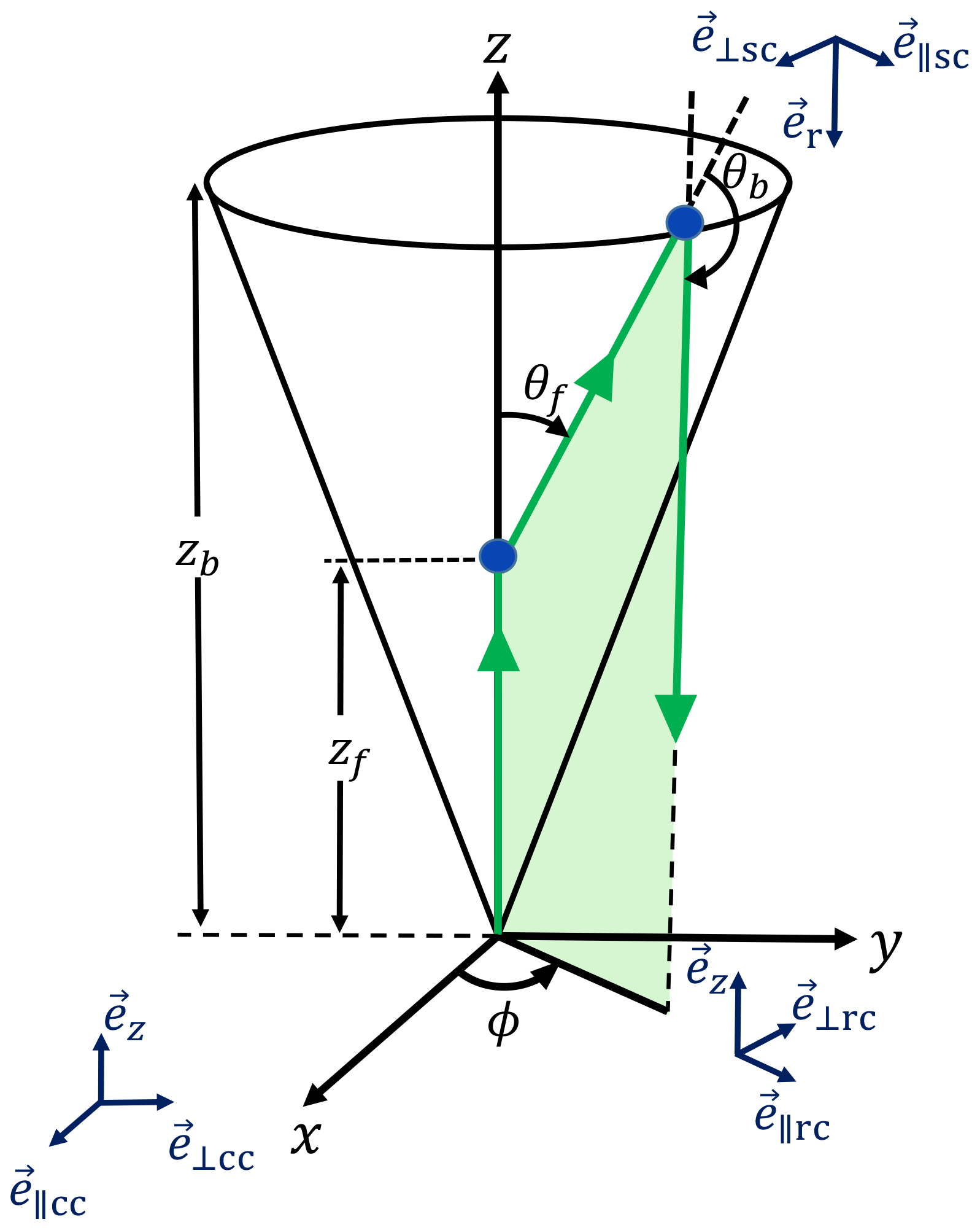
The Stokes vector describing the resulting polarization state with respect to the initial coordinate system, which we relate to the laser beam polarization state, can be obtained as follows:
Alin denotes the Stokes vector for the 100 % linearly polarized laser pulses, associated with the initial laser polarization plane (e∥cc, e⟂cc, ez). The transformation matrix Bcc→rc(ϕ) enables the transition from the Cartesian coordinate system (cc, e∥cc, e⟂cc, ez coordinates in Fig. 1) to the ϕ-rotated system (rc, e∥rc, e⟂rc, ez coordinates) followed by the scattering of the incident wave front. P represents the single scattering matrix defined for an isotropic media (Zege and Chaikovskaya, 2000). The matrices P(θf) and P(θb) denote the forward and backward scattering. The transformation matrix Bsc→cc finally enables the transition from the scattering-coordinate system (sc, e∥sc, e⟂sc, er coordinates in Fig. 1) to the original Cartesian system (cc) (Wandinger, 1994).
From the Stokes vector we can extract the co- and cross-polarized lidar signal components S∥ and S⟂. In Fig. 2b, the computed azimuthal patterns (in the backscatter plane orthogonal to the z axis in Fig. 1) of the co- and cross-polarized signal components for scattering angles from 170 to 180∘ are shown for four different droplet sizes. Those azimuthal patterns can be observed with imaging polarization lidars, which are supplied with a charged coupled device matrix as a photo-receiving element (Roy et al., 2004). But a common lidar receiver collects the scattered light over the entire azimuthal range and stores it as one signal. However, by selecting a certain receiver FOV, we define the range of scattering angles θf and θb that a lidar can detect in the multiple scattering regime, and by measuring lidar return signals at different FOVs and thus for different ranges of θf and θb, a way is opened to derive information about the droplet sizes as emphasized in Fig. 2a–d. This is the basic idea of combining lidar measurements at different FOVs to retrieve the effective radius of the droplets and, in the next step, further cloud properties as will be described in Sect. 4.

Figure 2(a) Normalized scattering matrix element P11 (normalized to the maximum at 0∘ scattering angle) as a function of forward scattering angle θf for four droplet effective radii (given as numbers), (b) azimuthal patterns (computed with the MS model for the entire range of azimuthal angles from 0 to 2π; see Fig. 1) of the co-polarized ∥ and the cross-polarized ⟂ signal components at scattering angles θb between 170 and 189.5∘ for the different droplet diameters, (c) droplet linear depolarization ratio with the lidar signal components S⟂ and S∥ (obtained from azimuthal integration over the range from ϕ=0–2π in b) as a function of the backscattering angle θb from 174∘ to 180∘ for the four droplet sizes, and (d) scattering matrix element P11(θ) at θf (in a) multiplied by the depolarization ratio at (in c).
From the two observed lidar signal components, S⟂ and S∥ backscattered at height zb, the so-called volume or, in the case of dense water clouds, droplet linear depolarization ratio defined as
is obtained. After forward scattering, the laser photons are backscattered at a certain backscatter angle θb. The dependence of the depolarization ratio on the backscatter angle θb is shown in Fig. 2c for the four droplet effective radii. It can be seen that the depolarization ratio increases to considerable values when the scattering angle deviates from 180∘. This sensitivity of the non-180∘ backscattering angle θb on light depolarization and the strong forward scattering peak in Fig. 2a are the features used in the dual-FOV polarization lidar technique to retrieve the basic cloud microphysical properties. Figure 2a, c, and d provide an impression of the sensitive impact of cloud droplet size on measurable lidar quantities and thus suggest again that polarization lidars operated at two FOVs have the potential to derive Re and subsequently also the cloud extinction coefficient α. Both Re and α are closely linked to the cloud droplet number concentration Nd (see Eq. 6). The relationship between MS-induced light depolarization measured at several FOVs and the cloud droplet size characteristics has already been illuminated and discussed in previous studies (Veselovskii et al., 2006; Roy et al., 2016). In the next sections, we will show that a dual-FOV polarization lidar can already provide trustworthy information about the size and extinction coefficient in the cloud base region of liquid water clouds.
To emphasize the dominating impact of the receiver FOV on the measured multiple scattering effects let us, at the end of this subsection, compare the influence of the laser beam width and divergence, receiver telescope area, and the receiver field of view on the observable cloud volume. In the case of a receiver FOV of 1 mrad, the lidar sees or observes a geometrical cross section (circular area in the horizontal plane at cloud base height zbot) of about 0.8, 7, and 20 m2 for a cloud with base height at 1, 3, and 5 km, respectively. The observable cross sections increase to about 3, 28, and 80 m2 when using a 2 mrad FOV. In contrast, in the case of a 30 cm receiver telescope (and a theoretical FOV of 0 mrad), the monitored circular cloud area at the cloud base is less than 0.1 m2. Also, the divergence of the laser beam (0.1 to 0.2 mrad) has only a minor impact on the amount of backscattered photons (and MS effects). The illuminated cloud cross section at cloud base is always < 1 m2 for a cloud base height of < 5 km. So, the FOV clearly determines the cloud volume (geometrical cross section at cloud base times 50–100 m laser beam penetration depth into the cloud) available for MS cloud studies with lidar.
3.3 Multiple scattering model
After presenting the principle relationship between the measured linear depolarization ratio, forward scattering, and droplet size, next we introduce the multiple scattering model used to develop our retrieval method presented in Sect. 4. The simulation model allows us to simulate realistic cloud scenarios with varying cloud height, droplet number concentration, cloud extinction coefficient, and droplet size distribution and the resulting co- and cross–polarized lidar signal components S∥ and S⟂ for given lidar configuration parameters such as laser beam divergence and receiver FOV.
In several articles, the radiative transfer problem of polarized light undergoing multiple scattering in an optically dense medium has been analytically addressed, and several solutions have been proposed and tested (Zege et al., 1995; Zege and Chaikovskaya, 1999, 2000). The so-called small-angle approximation is used. This solution is justified in the case of a narrow and pronounced forward scattering peak of the droplet scattering phase function which in turn is the case when the droplet size (on the order of 5–20 µm) is large compared to the laser wavelength (532 nm). Such an elongated forward-phase-function medium allows a simplification of Green's matrix. The vector equation can thus be split into a system of scalar-like equations which are simpler and include less integral terms than the original ones and can thus be solved by using well developed radiative-transfer-equation techniques.
The Stokes vector A has the general form and the Stokes vector is in the case of linearly polarized laser pulses (in x direction in Fig. 1) in Eq. (7).
The first element of the Stokes vector is the light intensity I which satisfies the radiative transfer equation using the single scattering matrix element P11(θ) (shown after normalization in Fig. 2a). The Q component of the Stokes vector describes the linear polarization and satisfies the same equation but with the “modified” angular scattering function that equals with the sign “+” for the forward and “−” for backward scattering. P22 and P33 are also elements of the scattering matrix P. In this way, the Stokes vector components can be solved separately as a scalar radiative transfer problem (Zege and Chaikovskaya, 2000). The more elongated the phase function, the more accurate the solution. This solution is not restricted to single and double scattering events. It simulates multiple forward scattering processes and one backscattering process. The approach offers high accuracy for optical depths up to 5 together with high computing efficiency (Chaikovskaya, 2008). The authors emphasized the potential of the model for developing new retrieval techniques.
The modeled components I and Q enable the calculations of the cross- and co-polarized returns S⟂(zb) and S∥(zb) for backscatter height zb within a liquid-water cloud layer,
The geometrical vector required to solve Eqs. (9) and (10) provides all necessary information about the lidar configuration, such as the full divergence angle of the laser beam Θldiv, the beam diameter dlb, the FOV full divergence angle of the receiver Θfov, the diameter of the primary receiver telescope dm1 and its respective secondary mirror shadow dm2sd. The atmospheric state vector provides the cloud information, i.e., cloud extinction coefficient α(zb) (assumed as the scattering coefficient) and effective radius Re at height zb.
The linear depolarization ratio according to Eqs. (8)–(10) is then given by
3.4 Model quality check: comparison with ECSIM Monte Carlo simulations and CALIPSO multiple scattering observations
We investigated to what extent the MS model used is able to simulate real-world polarization lidar observations and thus can be used to develop new lidar analysis methods with a focus on clouds. We compared our simulations with results obtained with the Monte Carlo simulation model ECSIM (EarthCARE Simulator) (Donovan et al., 2015, 2010) and observations with the CALIPSO (Cloud–Aerosol Lidar and Infrared Pathfinder Satellite Observation) lidar (Hu et al., 2007). EarthCARE (Earth Clouds, Aerosols and Radiation Explorer) is a planned spaceborne lidar and radar mission, designed within a co-operation of the European Space Agency (ESA) and the Japan Aerospace Exploration Agency (JAXA) (Illingworth et al., 2015). Based on the 4×4 α–Re combinations (4 α(zb) values in the range from 5 to 26 km−1, 4 Re(zb) values in the range from 3 to 15 µm), we performed more than 200 different simulations for these 16 cloud scenarios by considering cloud penetration depths from 10 to 70 m (with step width of 10 m), two different FOVs of 0.5 and 2.0 mrad, and assuming a liquid-cloud layer with a cloud base height at 3000 m. We compared the obtained volume depolarization ratio with respective values simulated with the Monte Carlo simulation model ECSIM in Fig. 3a. As can be seen, our simulations (δ(our model)) are in good agreement with results of the sophisticated Monte Carlo model. Both models agree for most of the depolarization ratio, except for the largest penetration depth exhibiting values close to 0.1. On average the depolarization ratios obtained with ECSIM are larger than our values by 0.016. The small differences indicate that our method delivers a realistic picture of multiple scattering in liquid-water clouds. The growing disagreement for depolarization ratios >0.05 is caused by different assumptions and implementations regarding the considered narrow ranges of the small-angle forward scattering processes and the one wide-angle backscattering process in the different models.
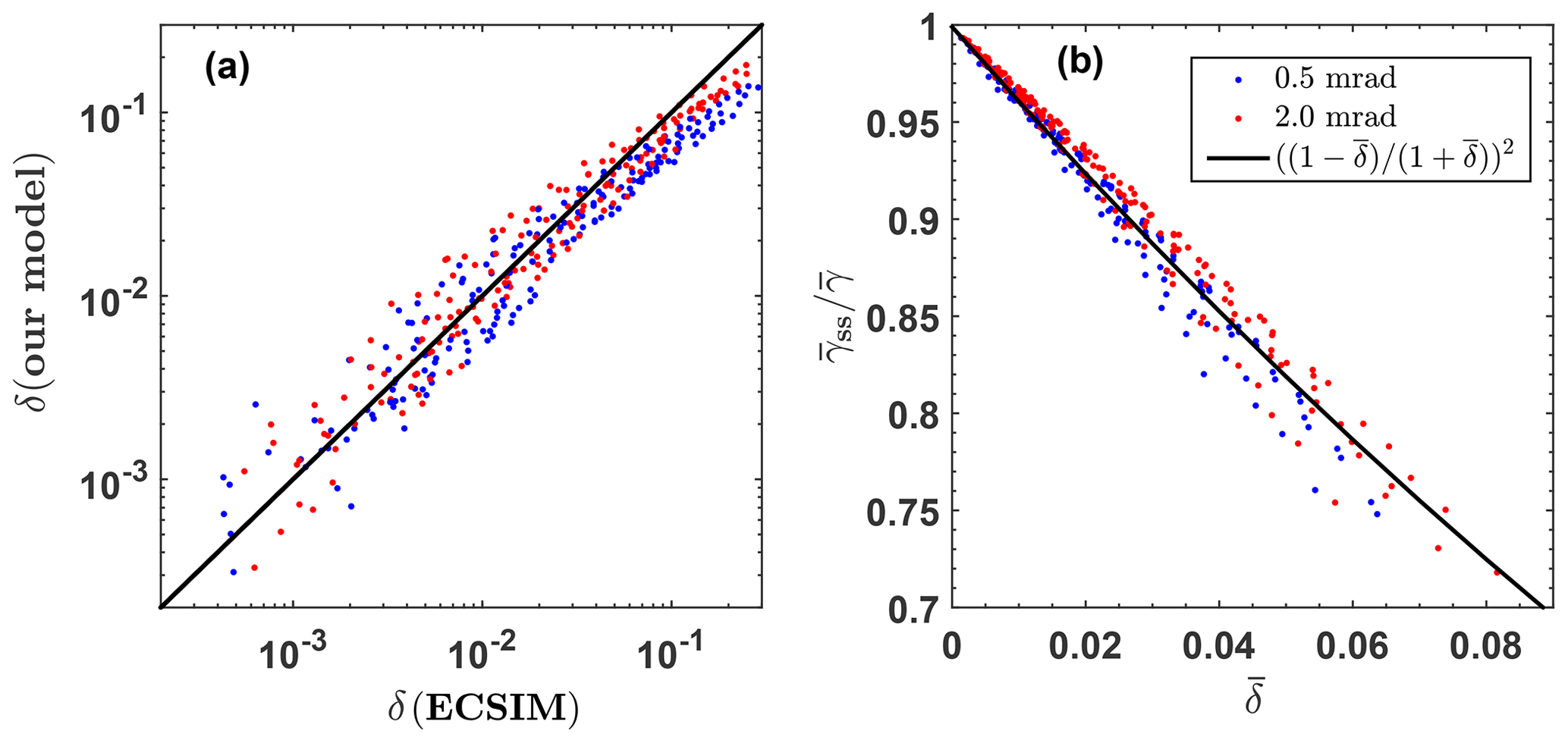
Figure 3(a) Comparison of the volume linear depolarization ratios δ(z) computed with our analytical MS model and computed with ESA's Monte Carlo model ECSIM (more details in the text, 1:1 line is given as solid diagonal line) and (b) comparison of our computations of the relationship between the single-scattering-to-total-scattering-attenuated-backscatter ratio and the cloud-integrated depolarization ratio (red and black circles) with the respective values for this relationship as retrieved from CALIPSO multiple scattering observations (solid black line). For the two different FOVs (0.5 mrad in blue, 2.0 mrad in red) 4×4 Re(zref) – α(zref) combinations are considered together with different cloud penetration depths Δzref from 10 to 70 m (with 10 m step width). All in all more than 200 simulations are included in each of the panels (a) and (b).
In a second approach, we compared our simulations with CALIPSO polarization lidar observations. Hu et al. (2007) investigated the relationship between the ratio of the total, cloud-integrated lidar return signal (from cloud top to base in the case of the CALIPSO lidar) to the one caused by single scattering ( caused by one backscattering process) and the respective cloud-integrated linear depolarization ratio . This study was based on observations with ground-based and spaceborne lidars supported by sophisticated Monte Carlo simulations of the multiple scattering impact on the observed cloud lidar returns. By performing a polynomial regression analysis to all observations they found the following best matching relationship:
The measured cloud-integrated CALIPSO lidar signal results from single plus multiple scattering events and corresponds to the respective cloud-integrated depolarization ratio for a given receiver FOV full angle Θ.
In Fig. 3b, the relationship presented by Hu et al. (2007) is shown as a solid black line. As can be seen, our individual simulations for the two FOVs (red and black circles) are in good agreement with Eq. (12) (black solid line in Fig. 3b), which again corroborates that our model describes well the link between cloud multiple scattering and light depolarization.
Based on simulations, the goal is to establish a method that allows us to retrieve Re and α from measured δ values at two FOVs, and afterwards to determine wl and Nd by means of Re and α. Therefore a large number of polarization lidar measurements for the full range of observable parameters were simulated with the MS model and formed the basis for the development of the new dual-FOV lidar measurement and data analysis concept.
To generate the input scenes, first the vertical profiles are computed and for this we assume that the cloud system develops at subadiabatic equilibrium, as first proposed by Albrecht et al. (1990). Recent experimental (Foth and Pospichal, 2017; Merk et al., 2016) and modeling studies (Barlakas et al., 2020) have shown that this assumption is appropriate to be applied in remote-sensing retrieval methods (Donovan et al., 2015). Such an subadiabatic system considers a reduction in the water content, compared to the adiabatic one, due to evaporation triggered by the entrainment of drier air masses caused by downward transport from above the cloud top.
Our data analysis scheme introduced below will deliver the cloud microphysical products for a height zref that is 50–100 m above the cloud base height zbot. The respective cloud penetration depth for laser light pulses is defined as
For convenience, we use Δzref=75 m in the following discussion. Following the methodological approach as outlined by Donovan et al. (2015), we assume that the cloud droplet number concentration Nd (Eq. 6) is height-independent and the liquid water content wl(z) increases linearly with height (see Fig. 4). The profile of the liquid-water content (Eq. 4) can thus be expressed by
with the gradient of the liquid-water content for subadiabatic cloud conditions and the column depth
Cloud droplets form at cloud base and then grow by water uptake at supersaturation conditions in updraft regions. According to Eqs. (4) and (14) we can write
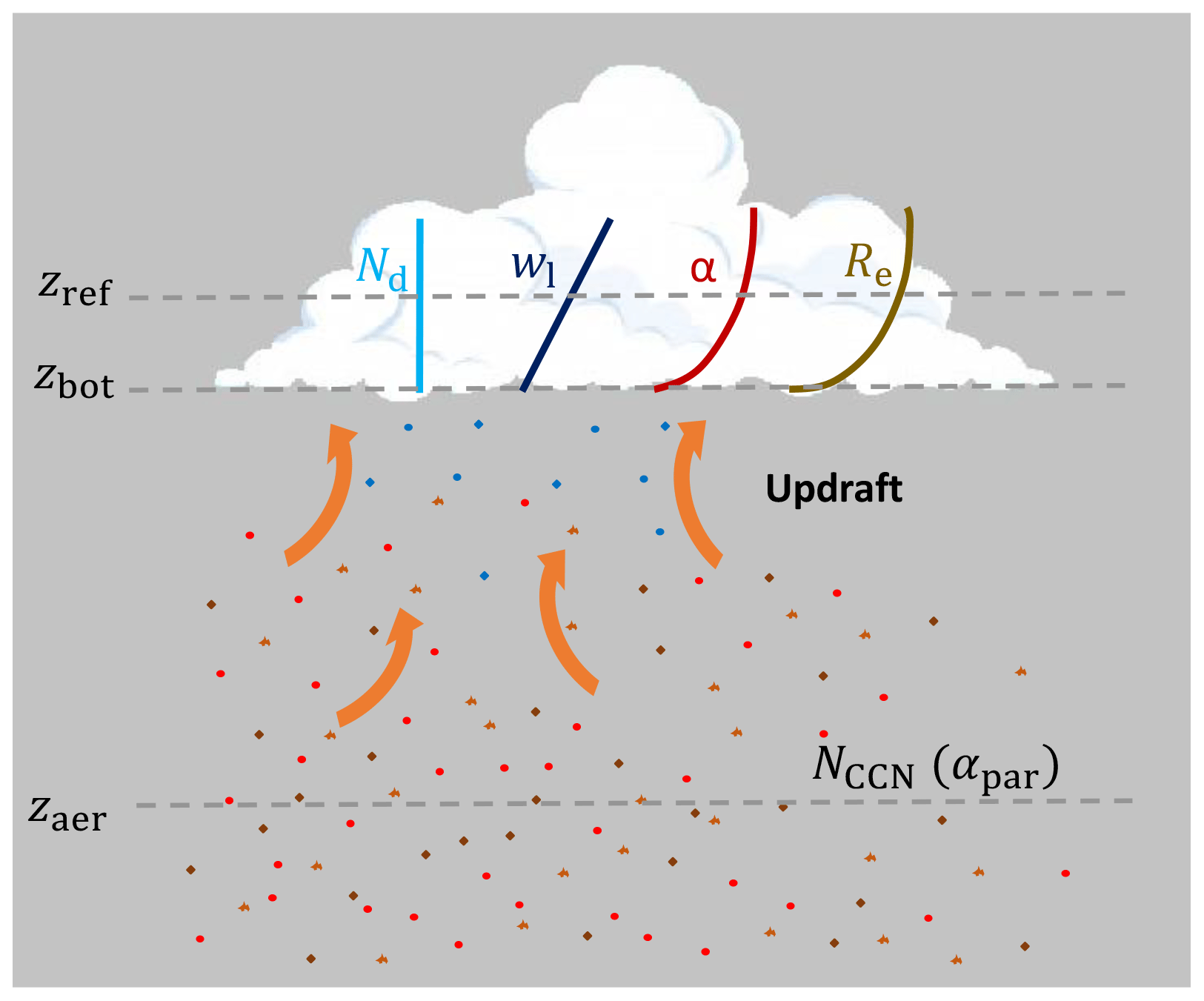
Figure 4Illustration of the overall concept to investigate aerosol–cloud interaction by combining observations of cloud microphysical properties at height zref 50–100 m above the cloud base at zbot with aerosol properties (particle extinction coefficient αpar, cloud condensation nucleus concentration NCCN) measured at height zaer several hundreds of meters below the cloud base. The indicated height profiles of cloud microphysical properties are used in the simulations to develop the new cloud retrieval scheme. Subadiabatic conditions in the lowest part of the cloud layer are assumed with an height-independent droplet number concentration Nd(z) and a linearly increasing liquid-water content wl(z). The profiles of the cloud extinction coefficient α(z) and the droplet effective radius Re(z) are then computed with Eqs. (21) and (18), respectively. All cloud parameters are zero at cloud base.
By using Eqs. (6) and (16) and forming the ratio ΓlΔz∕Nd we obtain
and for Re(z)
Further treatment leads to the link between Re(z) and Re(zref),
The Re(z) profile is shown in Fig. 4.
To obtain the profile of the cloud extinction coefficient α(z) used in the simulations we combine Eqs. (16) and (18),
Rearrangement yields
Finally, we can write
The profile of α(z) is sketched in Fig. 4 as well.
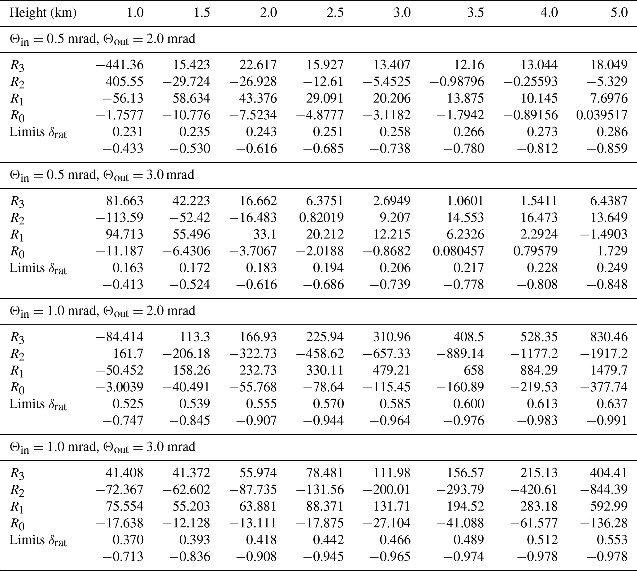
We used then the profiles in Fig. 4, described by Eqs. (6), (14), (18), and (21), to simulate the corresponding cross- and co-polarized lidar backscatter returns and the volume depolarization ratio (Eq. 11). We performed computations at two receiver FOVs for 720 different cloud scenarios (defined by the state vector X) by using Eqs. (9)–(10). The input parameters (10 values for α(zref), 9 values for Re(zref), and 8 cloud base altitudes zbot) are given in Table 1. Overall cloud depth was 200 m. Vertical resolution or step width in the computations was 7.5 m, which corresponds to the vertical resolution of the lidar observations introduced in Part 2 (Jimenez et al., 2020a).
Table 1Lidar and liquid-water cloud input parameters used in the simulations with the MS model.

Figure 5 shows the profiles of the linear depolarization ratios δin and δout for the inner and outer FOVs, i.e., for FOVin of 1 mrad and for FOVout of 2 mrad for four different profiles of the cloud extinction coefficient α and four different profiles of the effective radius Re of the droplets. The simulated cloud layer is at 3 km height. A monotonic increase in the volume linear depolarization ratio is visible because of the increasing contribution of multiple scattering processes to the amount of backscattered laser photons with increasing cloud penetration depths. With an increasing number of cloud droplets and thus increasing light extinction, the probability of multiple scattering and thus the strength of depolarization increase strongly.

Figure 5Simulated depolarization ratio profiles for (a) FOVin of 1 mrad, (b) FOVout of 2 mrad, and (c) profiles of the ratio δin(z)∕δout(z). α(zref) values are 5.2 km−1 (blue), 10.4 km−1 (red), 15.6 km−1 (green), and 26.0 km−1 (black) (see Table 1, zref=75 m above the cloud base at zbot=3 km). Different symbols indicate different simulated Re(zref) values (3.6 µm (triangle), 5.8 µm (circle), 7.9 µm (star), and 14.4 µm (square)). A clear dependence of Re(zref) on δin(z)∕δout(z) is visible up to about 100 m above the cloud base.
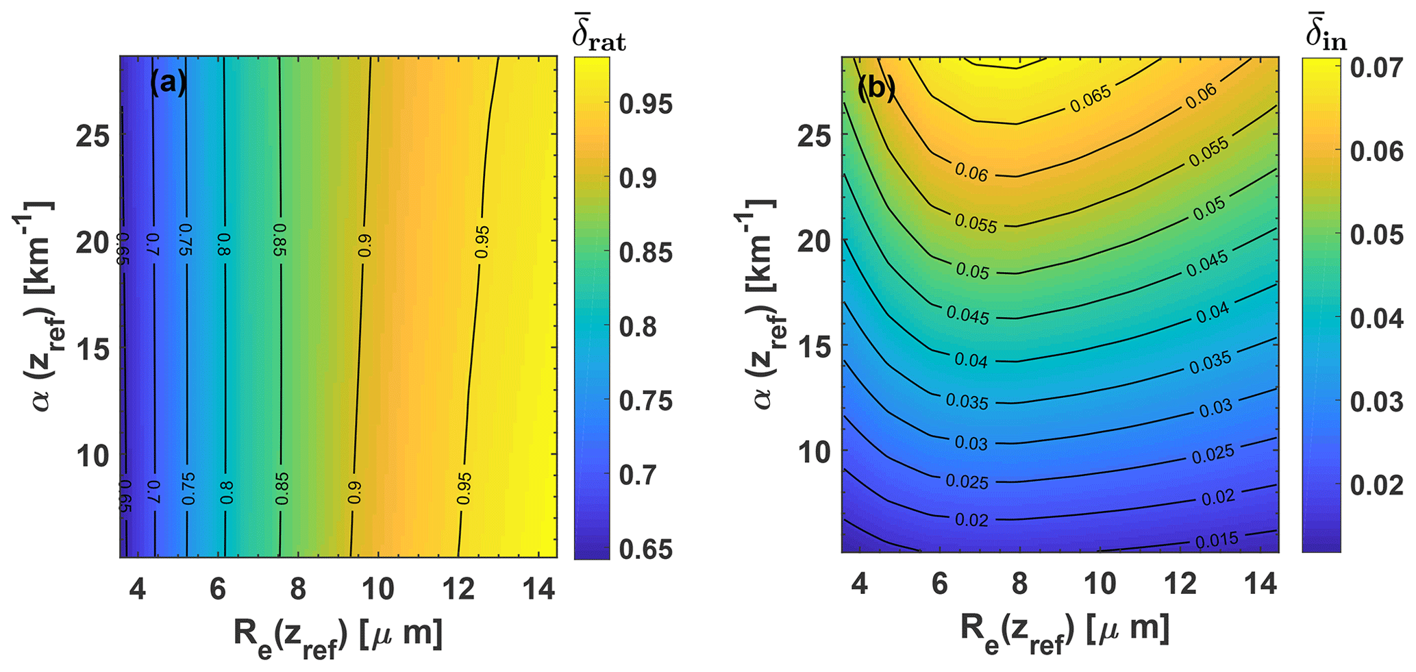
Figure 6(a) Ratio of depolarization ratios (see Eq. (25), integration height range of Δzref=75 m) as a function of droplet effective radius Re(zref) and cloud extinction coefficient α(zref). Cloud base zbot is at 3 km height, zref is thus at 3.075 km height. (b) Integrated depolarization ratio as a function of Re(zref) and α(zref). Isolines of in (a) show the strong dependence of on the effective radius. The isolines in (b) highlight the dominating influence of the extinction coefficient on . The figures are based on 720 simulated cloud scenarios for each of the FOVs of 1 and 2 mrad.
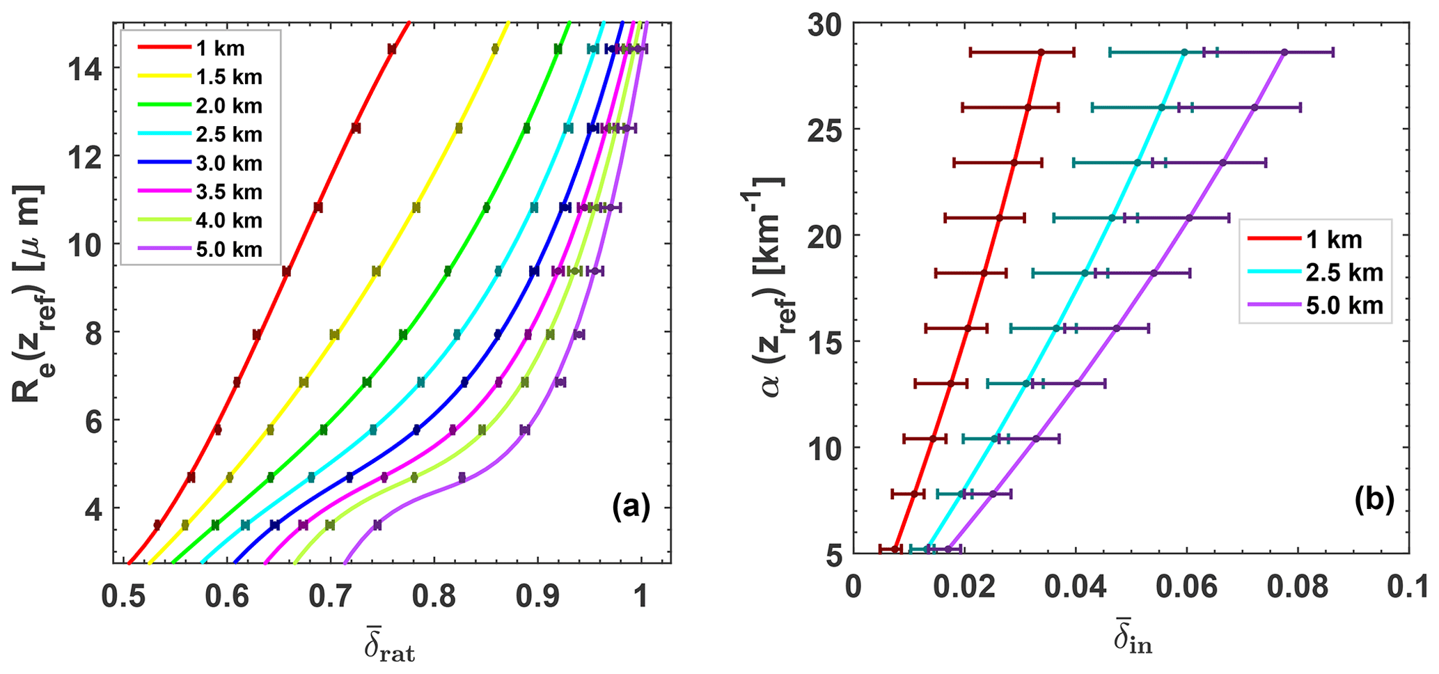
Figure 7(a) Droplet effective radius Re(zref) as a function of for Δzref=75 m and (b) relationship between the measured for FOV =1 mrad and cloud extinction coefficient α. Eight different cloud layers with base height zbot from 1 to 5 km height (given as numbers in the panels) are simulated in (a), and three different layers are simulated in (b). For each cloud layer (indicated by different colors) simulations with all combinations of Re–α profile pairs (in Table 1) are performed. The small bars in (a) indicate the range of possible δrat values for the whole range of α values at a given Re value, which indicate the very low influence of α on the Re retrieval (simulated α range is given in Table 1). A polynomial regression is applied to the mean values of . This regression analysis is performed for each of the eight cloud layers. The cubic model (Eq. 26) for each cloud layer is indicated as thick solid colored line. The bars in (b) indicate the range of possible δin values for a given α value. Here, the length of the bars indicate the relatively strong Re influence on the α(zref) retrieval (simulated Re range is given in Table 1). The respective regression analysis leads here to the thick solid lines calculated with Eq. (27).
The striking feature in Fig. 5 is the clear dependence of δin∕δout on the droplet effective radius Re(zref). In principle, we can show a similar figure by combining different backscatter signals measured with lidar at two different FOVs. However, the comparison of all these combinations clearly revealed that the optimum retrieval of the cloud effective radius (as shown in Fig. 5c) is only possible by means of the co- and cross-polarized signal components observed at different FOVs.
According to Fig. 5c it is recommended to use the lidar observations in the lowest part of the liquid-water cloud to retrieve the cloud microphysical properties. To obtain robust values of the cloud depolarization ratios at the two different FOVs (with low signal noise impact) we integrate, in the next step, the depolarization ratio from the cloud base to a fixed reference altitude (see Fig. 4),
and further define the dual-FOV ratio of depolarization ratios,
To check the sensitivity of the dual-FOV retrieval method to the selected pair of FOVs, we used the logarithmic derivative of the observables and the retrievable parameters, as proposed by Malinka and Zege (2007). We performed simulations with FOVs from 0.5 to 3.0 mrad and found that the highest sensitivity to the droplet effective radius is given for the case with the highest FOVout-to-FOVin ratio. However, the selection of FOVin of 1 mrad and FOVout of 2 mrad as used in the following was found to be sufficiently sensitive for liquid-water cloud studies and, on the other hand, a good compromise when keeping cloud inhomogeneities in consideration. Besides, this choice of FOVs allow us to upgrade our Polly systems (Engelmann et al., 2016) into a Dual-FOV Polarization lidar simply by adding one cross-polarized channel. This topic will be discussed in Part 2. The backscatter signals may be different for the two FOVs not only because of the different multiple scattering contributions, but also because of the differences in the amount of photon backscatter from different cloud cross sections and cloud volumes (defined by cloud height and FOV) as a result of inhomogeneities in cloud properties that may vary in the horizontal plane.
In Fig. 6, an overview of all simulations of and for 90 cloud scenarios (all possible combinations of cloud extinction and effective radii in Table 1) are shown for a cloud layer at zbot=3 km and FOVs of 1 and 2 mrad. As mentioned, the depolarization ratio values are integrated over the lowest 75 m of the cloud layer. Again, a clear dependence of on the effective radius Re at zref (75 m above the cloud base) is visible in Fig. 6a. The dominating impact of the cloud extinction coefficient on is shown in Fig. 6b.
In Fig. 7a, the relationship between and effective radius Re(zref) is presented for all cloud layers with base heights from 1 to 5 km and FOVs of 1 and 2 mrad. The horizontal bars indicate the influence of the cloud extinction coefficient for each of the simulated nine effective radii for the eight cloud layers. A polynomial regression is applied to each of the eight cloud simulation data sets and the respective cubic polynomial fits (Eq. 26) are shown as colored curves in Fig. 7a. To perform the regression the mean values of over α were considered.
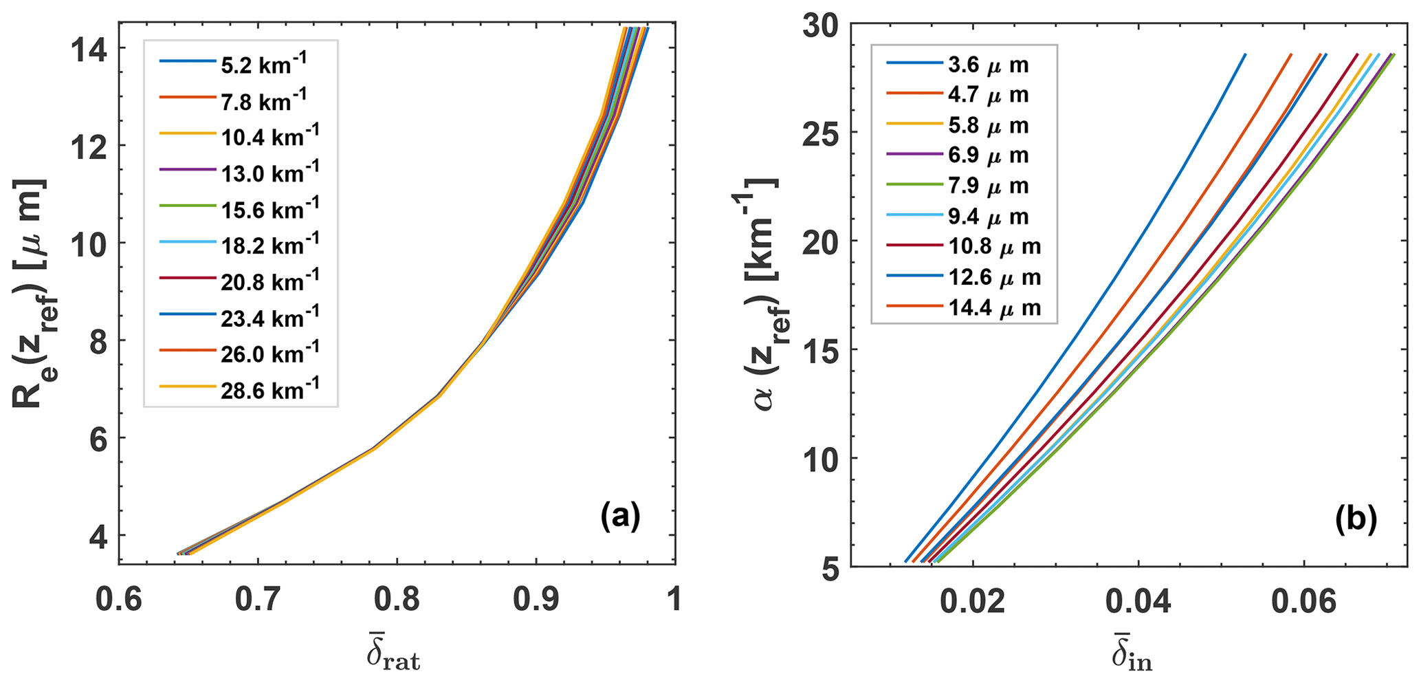
Figure 8Two-step approach to derive Re(zref) and α(zref) from and for a liquid cloud layer with zbot=3 km and zref=3.075 km. In the first step (a), is used to determine Re(zref) by means of Eq. (26), and in the second step (b), and Re (from step 1) are used to determine α(zref) with Eq. (27). In (a), all simulations with all available combinations of Re–α profile pairs are shown to indicate the low impact of α (given as numbers) on the retrieval. In (b), the relationship between and α for nine Re values (given as numbers) are shown to indicate the comparably large influence of Re on the α retrieval.
Equation (26) is now used in our dual-FOV method to derive the droplet effective radius Re(zref) from the measurements of for the integration length Δzref=75 m:
The polynomial coefficients R0, R1, R2, and R3 are given in Table 2. For a given cloud base altitude, we obtained the appropriate curve by interpolating the two nearest curves (computed by means of the Table 2 values) for the adjacent heights.
Table 2Polynomial coefficients used in the computation of Re with Eq. (26).
In the second step of the retrieval, the cloud extinction coefficient α(zref) is determined by using the derived effective radius and the measured integrated depolarization ratio inserted in the quadratic polynomial fit,
The coefficients α0(Re,zbot), α1(Re,zbot), and α2(Re,zbot) are obtained from a polynomial regression analysis applied to each simulation data set for a given cloud layer characterized by zbot and Re(zref) as well as the given inner FOV. Figure 7b shows the relationship between the different parameters.
The two-step retrieval is finally explained again in Fig. 8 for a cloud layer with cloud base height of 3 km, zref at 75 m above cloud base height, and FOVs of 1 and 2 mrad. To show again the low dependency of on cloud extinction, all 10 simulations with α(zref) values from 5.2 to 28.6 km−1 are presented. A clear relationship between and Re(zref) according to Eq. (26) is given. Figure 8b is the basis for the second step of the retrieval. Here, the polynomial fits (Eq. 27) of the α(zref) vs. simulations are used and shown in Fig. 8b for the nine discrete effective radius values in Table 1. Thus, to avoid large errors in the α(zref) retrieval, Re(zref) from step 1 is used to select the right curve for the α(zref) determination.
Finally, after the derivation of the droplet extinction coefficient α(zRef) and the droplet effective radius Re(zref) as independent variables, we can compute the liquid-water content wl(zref) with Eq. (4) and the droplet number concentration Nd(zref) with Eq. (6), in the same way as presented by Schmidt et al. (2013, 2014).
The polynomial coefficients to retrieve Re(zref), in Table 2, for the pair of FOVs 0.1 and 2.0 mrads, and the matrices containing the values of for given values of Re(zref) and α(zref), to generate the quadratic polynomials for the second step of the retrieval, i.e to derive α(zref), from the obtained Re(zref) and the observation of , can be found in Jimenez et al. (2020b).
With Eqs. (26) and (27) the retrieval of the effective radius and extinction coefficient is possible. In this section, we illuminate the underlying uncertainties in the retrieval of these cloud parameters. First, we consider the assumption about the vertical structure of the cloud, i.e., a subadiabatic cloud system. Whether the cloud conditions are adiabatic or subadiabatic is not an important issue as in both systems the water content increases linearly with height. When the real water content or number concentration profiles differ slightly from our assumptions (of a linearly increasing wl and height-independent Nd), the monotonic form of the simulated observables ( and ) as a function of droplet size and extinction coefficient (in Fig. 7) would still hold for cases in which the vertical profiles differ from the theoretical ones, as long as the height-averaged values are the same. However, in cases with very different profiles, e.g., in cases with vertically homogeneous cloud properties, the retrieval curves may change. As a consequence, the interpretation of cloud observations, e.g., during downdraft situations, should be interpreted with care because our basic assumption of a linearly increasing wl and height-constant Nd may be no longer valid.
The retrieval of the effective radius Re(zref) of the cloud droplets needs the ratio of depolarization ratios and the cloud base height zbot as input. The relationship between Re(zref) and is also a function of the cloud extinction coefficient α(zref). We can estimate the uncertainties caused by the uncertainty in the measurement by calculating
and by taking half of the respective uncertainty bars.
Systematic retrieval uncertainties arise from the use of the model (polynomial functions in Fig. 7), the uncertainties in the determined cloud base height Δzbot (we assume ±15 m), and the influence of the cloud extinction coefficient (the uncertainty is denoted here as Δα and given by the range of values in Table 1 from 5.2 to 28.6 Mm−1). From the extended error simulations and from the analysis with real (observational) data we conclude that
On average, input uncertainties may partly cancel out and the mean uncertainty is given by
The influence of measurement uncertainties on the retrieval of α(zref) is estimated by considering the standard deviation in the computation,
In a similar way to that described above for the systematic uncertainty in Re, we estimated σsys,α with Δzbot±15 m and by using ΔRe according to Eq. (31) in the second retrieval step to obtain α(zref). Again, from many simulations we concluded that
The overall mean systematic uncertainty may be given by
6.1 Lidar-derived aerosol properties
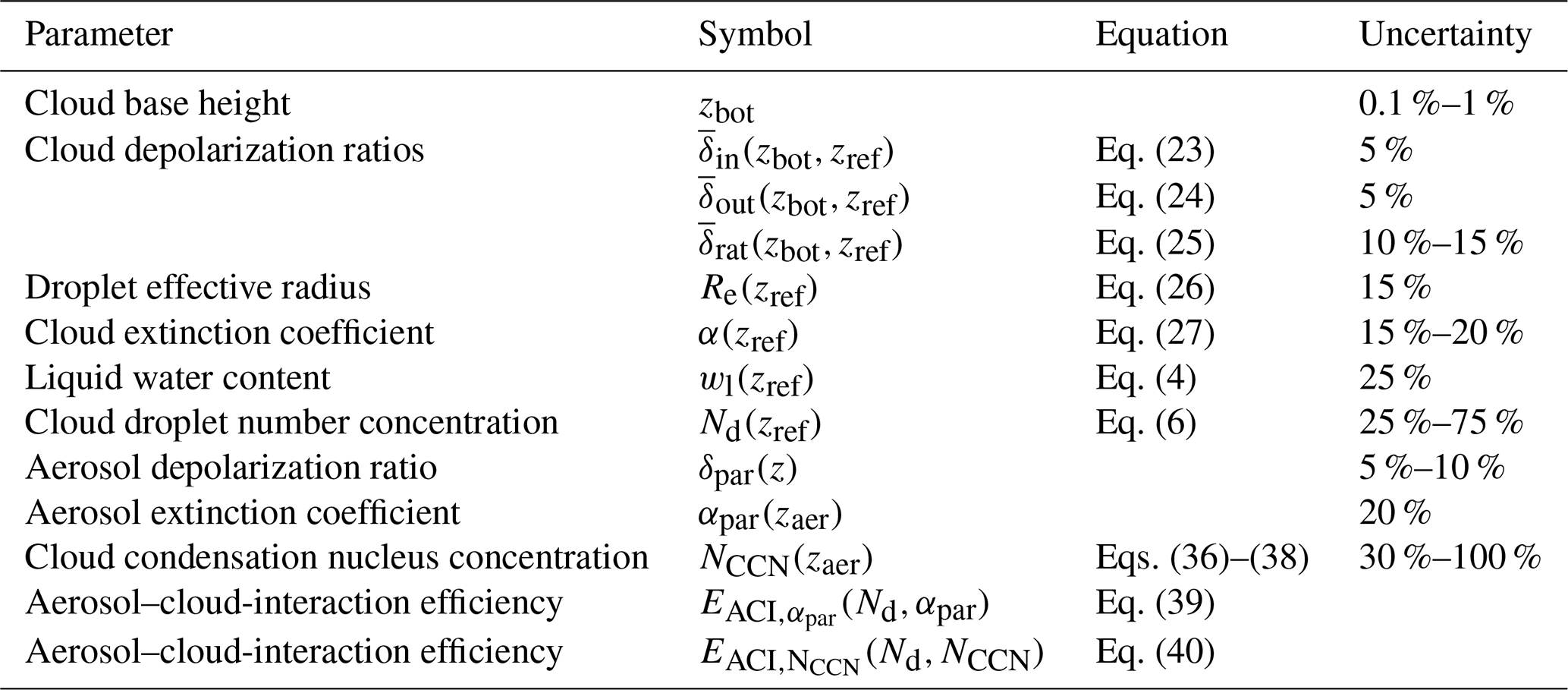
For completeness of the theoretical Part 1, we briefly introduce the aerosol parameters needed for the ACI studies. Examples of aerosol observations with the multiwavelength polarization Raman lidar Polly (portable lidar system) (Engelmann et al., 2016) used in Part 2 and upgraded to a dual-FOV polarization lidar can be found in Baars et al. (2016) and Hofer et al. (2017, 2020). The sketch in Fig. 4 illustrates our overall concept of lidar-based ACI studies. The aerosol parameters are measured with the lidar at the smaller FOV (FOVin) several hundreds of meters below the cloud base. The cloud- and ACI-relevant aerosol proxies are the particle extinction coefficient αpar(z) and the cloud condensation nucleus concentration NCCN(z). The methodology to derive NCCN profiles from measurements of particle optical properties is outlined in Mamouri and Ansmann (2016). A brief summary of the method, denoted as the POLIPHON (Polarization Lidar Photometer Networking) method, is given here.
A specific problem in ACI studies is the retrieval of the particle backscatter and extinction profiles below extended liquid-water cloud layers in the first step. The required calibration of the lidar profiles in clear air (in pure Rayleigh scattering conditions), i.e., in the upper troposphere and lower stratosphere, is then not possible. In these cases with aerosol backscatter signals up to cloud base height zbot only, the so-called lidar constant is required in the retrieval of aerosol properties. The determination of the lidar constant (considering all instrumental constants, such as laser pulse energy and receiver telescope area, in the basic lidar equation) following the procedure of Wiegner and Geiß (2012) is performed during cloud-free situations before or after the passage of the cloud fields or during periods with cloud holes so that clear air layers (Rayleigh scattering regime) are available for the lidar calibration. Subsequently, the determined lidar constant is used during the cloudy periods in the data analysis to retrieve the backscatter coefficient profiles up to the base of the optically dense water clouds again following the procedure of Wiegner and Geiß (2012).
By means of height profiles of the aerosol particle depolarization ratio and the particle backscatter coefficient, the POLIPHON data analysis separates particle backscatter and extinction contribution of the three basic aerosol types (marine aerosol, mineral dust, anthropogenic haze). The aerosol-type-dependent 532 nm extinction coefficients below the cloud base zbot are then converted into particle number concentrations and respective CCN concentrations (for a water supersaturation level of 0.2 % or relative humidity over water of 100.2 %) as described by Mamouri and Ansmann (2016).
For pure marine conditions, we obtain NCCN from αpar by using the following conversion:
with NCCN per cubic centimeter (cm−3) and αpar in units of inverse megameter (Mm−1). For urban haze conditions (central European pollution conditions), we apply
and for desert dust
The NCCN values assume that all dry particles with radius > 50 nm (marine, urban) and > 100 nm are potential cloud condensation nuclei. The parameterization holds for an ambient relative humidity of 60 % relative humidity for continental fine-mode aerosol and 80 % relative humidity in the case of marine particles. Respective water-uptake effects by aerosol particles are considered and corrected in Eqs. (36) and (37). In the case of hydrophobic dust particles, no water uptake effect is considered and corrected.
The uncertainty in the basic aerosol-type-dependent extinction coefficients and in the retrieved NCCN values is on the order of 20 % and 50 %–100 %, respectively. However, aircraft comparisons (Düsing et al., 2018; Haarig et al., 2019) and long-term field studies at a central European background station (Schmale et al., 2018) revealed that the uncertainty is typically on the order of 50 % for lidar-derived CCN estimates. It should be emphasized at the end that the Raman lidar Polly permits the retrieval of profiles of the water-vapor mixing ratio and relative humidity (RH) (Dai et al., 2018) so that, in principle, actual RH measurements are available for the required aerosol water uptake effects in the NCCN conversion procedure as described by Mamouri and Ansmann (2016)
6.2 Aerosol–cloud-interaction (ACI) parameter
The study of the influence of aerosol particles on liquid-water cloud evolution and cloud microphysical properties is based on two ACI parameters defined as follows (Feingold et al., 2001; McComiskey et al., 2009; Schmidt et al., 2013, 2014):
and
The so-called nucleation-efficiency parameter describes the relative change of the cloud droplet number concentration Nd with a relative change in the particle extinction coefficient αpar. Correspondingly, characterizes the relative increase in Nd with a relative increase in the cloud condensation nucleus concentration NCCN. The higher the ACI value, the stronger the impact of the observed aerosol conditions on the cloud microphysical properties.
Table 3Overview of the cloud and aerosol retrieval procedure (step-by-step data analysis). The data analysis starts with a precise determination of the cloud base height zbot. The cloud products are given at the reference height zref, 75 m above the cloud base height zbot. In the estimation of the ACI efficiency, particle extinction and cloud condensation nucleus concentration at zaer, usually several hundreds of meters below the cloud base, are considered.
We presented a new polarization-based lidar approach to derive microphysical properties of pure liquid-water clouds. Extended simulations with a multiple scattering model were performed regarding the relationship between cloud microphysical and light-extinction properties and the cloud depolarization ratio measured with lidar at two different FOVs. These simulations served as the basis for the development of the new dual-FOV polarization lidar method. An extended error analysis was performed as well. The new dual-FOV polarization lidar technique can be combined with the POLIPHON method, which allows the profiling of CCN concentrations below the cloud base. In Table 3, the full data analysis scheme of the dual-FOV polarization lidar is shown. All steps of the data analysis procedure from the determination of the cloud microphysical properties and the aerosol proxies to the ACI parameters are listed.
In our follow-up article (Jimenez et al., 2020a), we describe how we implemented the novel dual-FOV polarization lidar technique into a Polly instrument which is now being used in a long-term field campaign in Punta Arenas, southern Chile, at the southern-most tip of South America. The field site is surrounded by the Southern Ocean. Pristine marine conditions prevail. Continental and especially anthropogenic aerosol sources usually play a negligible role regarding their influence on cloud evolution and properties in this region of the world. We present two case studies of this campaign in Part 2. Case 1 is used to explain the full aerosol and cloud data analysis scheme in detail. This case study includes an uncertainty discussion and comparisons with alternative approaches to derive cloud microphysical properties such as the single-FOV polarization lidar technique (Donovan et al., 2015). Based on case 2, the potential of the new lidar technique to improve ACI studies in the case of liquid-water clouds is highlighted.
The simulation products to perform the retrieval of microphysical properties can be found at https://doi.org/10.5281/zenodo.4107137 (Jimenez et al., 2020b).
CJ and AA prepared the manuscript. CJ developed the method and performed the MS simulations. The analytical MS code was developed and provided by AM. DD performed the simulations with the ECSIM MS model. AA, RE, DD, AM, JS, and UW contributed to the design of the simulations study and to the discussion of the results.
The authors declare that they have no conflict of interest.
This article is part of the special issue “EARLINET aerosol profiling: contributions to atmospheric and climate research”. It is not associated with a conference.
The authors would like to thank the TROPOS lidar team members for their support and numerous fruitful discussions during the last 5 years.
This research has been supported by the DAAD/Becas Chile (grant no. 57144001) and the ACTRIS Research Infrastructure (EU H2020-R&I) (grant no. 654109).
The publication of this article was funded by the
Open Access Fund of the Leibniz Association.
This paper was edited by Eduardo Landulfo and reviewed by two anonymous referees.
Albrecht, B. A., Fairall, C. W., Thomson, D. W., White, A. B., Snider, J. B., and Schubert, W. H.: Surface-based remote sensing of the observed and the adiabatic liquid water content of stratocumulus clouds, Geophys. Res. Lett., 17, 89–92, https://doi.org/10.1029/GL017i001p00089, 1990. a
Ansmann, A., Mamouri, R.-E., Hofer, J., Baars, H., Althausen, D., and Abdullaev, S. F.: Dust mass, cloud condensation nuclei, and ice-nucleating particle profiling with polarization lidar: updated POLIPHON conversion factors from global AERONET analysis, Atmos. Meas. Tech., 12, 4849–4865, https://doi.org/10.5194/amt-12-4849-2019, 2019.
Baars, H., Kanitz, T., Engelmann, R., Althausen, D., Heese, B., Komppula, M., Preißler, J., Tesche, M., Ansmann, A., Wandinger, U., Lim, J.-H., Ahn, J. Y., Stachlewska, I. S., Amiridis, V., Marinou, E., Seifert, P., Hofer, J., Skupin, A., Schneider, F., Bohlmann, S., Foth, A., Bley, S., Pfüller, A., Giannakaki, E., Lihavainen, H., Viisanen, Y., Hooda, R. K., Pereira, S. N., Bortoli, D., Wagner, F., Mattis, I., Janicka, L., Markowicz, K. M., Achtert, P., Artaxo, P., Pauliquevis, T., Souza, R. A. F., Sharma, V. P., van Zyl, P. G., Beukes, J. P., Sun, J., Rohwer, E. G., Deng, R., Mamouri, R.-E., and Zamorano, F.: An overview of the first decade of PollyNET: an emerging network of automated Raman-polarization lidars for continuous aerosol profiling, Atmos. Chem. Phys., 16, 5111–5137, https://doi.org/10.5194/acp-16-5111-2016, 2016. a
Barlakas, V., Deneke, H., and Macke, A.: The sub-adiabatic model as a concept for evaluating the representation and radiative effects of low-level clouds in a high-resolution atmospheric model, Atmos. Chem. Phys., 20, 303–322, https://doi.org/10.5194/acp-20-303-2020, 2020. a
Bissonnette, L. R., Bruscaglioni, P., Ismaelli, A., Zaccanti, G., Cohen, A., Benayahu, Y., Kleiman, M., Egert, S., Flesia, C., Schwendimann, P., Starkov, A. V., Noormohammadian, M., Oppel, U. G., Winker, D. M., Zege, E. P., Katsev, I. L., and Polonsky, I. N.: LIDAR multiple scattering from clouds, Appl. Phys. B, 60, 355–362, https://doi.org/10.1007/BF01082271, 1995. a
Bissonnette, L. R., Roy, G., and Roy, N.: Multiple-scattering-based lidar retrieval: method and results of cloud probings, Appl. Optics, 44, 5565–5581, 2005. a, b
Bissonnette, L. R., Roy, G., and Tremblay, G.: Lidar-Based Characterization of the Geometry and Structure of Water Clouds, J. Atmos. Ocean. Tech., 24, 1364–1376,https://doi.org/10.1175/JTECH2045.1, 2006.
Chaikovskaya, L.: Remote sensing of clouds using linearly and circularly polarized laser beams: techniques to compute signal polarization, in: Light Scattering Reviews, edited by: Kokhanovsky, A. A., Springer Praxis Books, Berlin and Heidelberg, Germany, 191–228, https://doi.org/10.1007/978-3-540-48546-9_6, 2008. a, b
Chaikovskaya, L. and Zege, E.: Theory of polarized lidar sounding including multiple scattering, J. Quant. Spectrosc. Ra., 88, 21–35, https://doi.org/10.1016/j.jqsrt.2004.01.002, 2004. a
Chaikovskaya, L., Zege, E., Katzev, I., Hirschberger, M., and Oppel, U.: Lidar returns from multiply scattered media in multiple-field-of-view and CCD lidars with polarization devices: comparison of semi-analytical solution and Monte Carlo data, Appl. Optics, 48, 623–632, 2009.
Dai, G., Althausen, D., Hofer, J., Engelmann, R., Seifert, P., Bühl, J., Mamouri, R.-E., Wu, S., and Ansmann, A.: Calibration of Raman lidar water vapor profiles by means of AERONET photometer observations and GDAS meteorological data, Atmos. Meas. Tech., 11, 2735–2748, https://doi.org/10.5194/amt-11-2735-2018, 2018. a
Donovan, D., Voors, R., van Zadelhoff, G.-J., and Acarreta, J.-R.: ECSIM Model and Algorithms Document, KNMI Tech. Rep.: ECSIM-KNMI-TEC-MAD01-R, available at: https://www.academia.edu/33712449/ECSIM_Model_and_Algorithms_Document (last access: 28 November 2020), 2010. a
Donovan, D. P., Klein Baltink, H., Henzing, J. S., de Roode, S. R., and Siebesma, A. P.: A depolarisation lidar-based method for the determination of liquid-cloud microphysical properties, Atmos. Meas. Tech., 8, 237–266, https://doi.org/10.5194/amt-8-237-2015, 2015. a, b, c, d, e, f, g, h, i, j
Düsing, S., Wehner, B., Seifert, P., Ansmann, A., Baars, H., Ditas, F., Henning, S., Ma, N., Poulain, L., Siebert, H., Wiedensohler, A., and Macke, A.: Helicopter-borne observations of the continental background aerosol in combination with remote sensing and ground-based measurements, Atmos. Chem. Phys., 18, 1263–1290, https://doi.org/10.5194/acp-18-1263-2018, 2018. a
Eloranta, E. W.: Practical model for the calculations of multiply scattered lidar returns, Appl. Optics, 37, 2464–2472, 1998. a
Engelmann, R., Kanitz, T., Baars, H., Heese, B., Althausen, D., Skupin, A., Wandinger, U., Komppula, M., Stachlewska, I. S., Amiridis, V., Marinou, E., Mattis, I., Linné, H., and Ansmann, A.: The automated multiwavelength Raman polarization and water-vapor lidar PollyXT: the neXT generation, Atmos. Meas. Tech., 9, 1767–1784, https://doi.org/10.5194/amt-9-1767-2016, 2016. a, b
Feingold, G., Remer, L., Ramaprasad, J., and Kaufman, Y.: Analysis of smoke impact on clouds in Brazilian biomass burning regions: An extension of Twomey's approach, J. Geophys. Res., 106, 907–922, https://doi.org/10.1029/2001JD000732, 2001. a
Foth, A. and Pospichal, B.: Optimal estimation of water vapour profiles using a combination of Raman lidar and microwave radiometer, Atmos. Meas. Tech., 10, 3325–3344, https://doi.org/10.5194/amt-10-3325-2017, 2017. a
Giannakaki, E., Kokkalis, P., Marinou, E., Bartsotas, N. S., Amiridis, V., Ansmann, A., and Komppula, M.: The potential of elastic and polarization lidars to retrieve extinction profiles, Atmos. Meas. Tech., 13, 893–905, https://doi.org/10.5194/amt-13-893-2020, 2020.
Grosvenor, D. P., Sourdeval, O., Zuidema, P., Ackerman, A., Alexandrov, M. D., Bennartz, R., Boers, R., Cairns, B., Chiu, J. C., Christensen, M., Deneke, H., Diamond, M., Feingold, G., Fridlind, A., Hünerbein, A., Knist, C., Kollias, P., Marshak, A., McCoy, D., Merk, D., Painemal, D., Rausch, J., Rosenfeld, D., Russchenberg, H., Seifert, P., Sinclair, K., Stier, P., van Diedenhoven, B., Wendisch, M., Werner, F., Wood, R., Zhang, Z., and Quaas, J.: Remote sensing of droplet number concentration in warm clouds: A review of the current state of knowledge and perspectives, Rev. Geophys., 56, 409–453, https://doi.org/10.1029/2017RG000593, 2018. a
Haarig, M., Walser, A., Ansmann, A., Dollner, M., Althausen, D., Sauer, D., Farrell, D., and Weinzierl, B.: Profiles of cloud condensation nuclei, dust mass concentration, and ice-nucleating-particle-relevant aerosol properties in the Saharan Air Layer over Barbados from polarization lidar and airborne in situ measurements, Atmos. Chem. Phys., 19, 13773–13788, https://doi.org/10.5194/acp-19-13773-2019, 2019. a
Hofer, J., Althausen, D., Abdullaev, S. F., Makhmudov, A. N., Nazarov, B. I., Schettler, G., Engelmann, R., Baars, H., Fomba, K. W., Müller, K., Heinold, B., Kandler, K., and Ansmann, A.: Long-term profiling of mineral dust and pollution aerosol with multiwavelength polarization Raman lidar at the Central Asian site of Dushanbe, Tajikistan: case studies, Atmos. Chem. Phys., 17, 14559–14577, https://doi.org/10.5194/acp-17-14559-2017, 2017. a
Hofer, J., Ansmann, A., Althausen, D., Engelmann, R., Baars, H., Abdullaev, S. F., and Makhmudov, A. N.: Long-term profiling of aerosol light extinction, particle mass, cloud condensation nuclei, and ice-nucleating particle concentration over Dushanbe, Tajikistan, in Central Asia, Atmos. Chem. Phys., 20, 4695–4711, https://doi.org/10.5194/acp-20-4695-2020, 2020. a
Hogan, R. J.: Fast Lidar and Radar Multiple-Scattering Models. Part I: Small-Angle Scattering Using the Photon Variance-Covariance Method, J. Atm. Sci., 65, 3621–3635, https://doi.org/10.1175/2008JAS2642.1, 2008. a
Holben, B. N., Eck, T. F., Slutsker, I., Tanré, D., Buis, J. P., Setzer, A., Vermote, E., Reagan, J. A., Kaufman, Y. J., Nakajima, T., Lavenu, F., Jankowiak, I., and Smirnov, A.: AERONET – a federated instrument network and data archive for aerosol characterization, Remote Sens. Environ., 66, 1–16, 1998.
Hu, Y., Vaughan, M., Liu, Z., Lin, B., Yang, P., Flittner, D., Hunt, B., Kuehn, R., Huang, J., Wu, D., Rodier, S., Powell, K., Trepte, C., and Winker, D.: The depolarization – attenuated backscatter relation: CALIPSO lidar measurements vs. theory, Opt. Express, 15, 5327–5332, 2007. a, b, c
Illingworth, A. J., Barker, H. W., Beljaars, A., Ceccaldi, M., Chepfer, H., Clerbaux, N., Cole, J., Delanoe, J., Domenech, C., Donovan, D. P., Fukuda, S., Hirakata, M., Hogan, R. J., Huenerbein, H., Kollias, P., Kubota, T., Nakajima, T., Nakajima, T. Y., Nishizawa, T., Ohno, Y., Okamoto, H., Oki, R., Sato, K., Satoh, M., Shephard, M., Velázquez-Blázquez, A., Wandinger, U., Wehr, T., and Zadelhoff, G.-J.: The EARTHCARE satellite: the next step forward in global measurements of clouds, aerosols, precipitation and radiation, B. Am. Meteorol. Soc., 96, 1311–1332, https://doi.org/10.1175/BAMS-D-12-00227.1, 2015. a
IPCC: Climate Change 2014: Synthesis Report, Contribution of Working Groups I, II and III to the Fifth Assessment Report of the Intergovernmental Panel on Climate Change, edited by: Core Writing Team, Pachauri, R. K., and Meyer, L. A., IPCC, Geneva, Switzerland, 151 pp., available at: https://www.ipcc.ch/pdf/assessment-report/ar5/syr/SYR_AR5_FINAL_full.pdf (last access: 28 November 2020), 2014. a
Jimenez, C., Ansmann, A., Donovan, D., Engelmann, R., Malinka, A., Schmidt, J., and Wandinger, U.: Retrieval of microphysical properties of liquid water clouds from atmospheric lidar measurements: Comparison of the Raman dual field of view and the depolarization techniques, Proc. SPIE, 10429, 1042907, https://doi.org/10.1117/12.2281806, 2017. a
Jimenez, C., Ansmann, A., Donovan, D., Engelmann, R., Schmidt, J., and Wandinger, U.: Comparison between two lidar methods to retrieve microphysical properties of liquid water clouds, EPJ Web Conf., The 28th International Laser Radar Conference, June 2017, Bucharest, Romania, 17601032, https://doi.org/10.1051/epjconf/201817601032, 2018. a
Jimenez, C., Ansmann, A., Engelmann, R., Donovan, D., Malinka, A., Seifert, P., Radenz, M., Yin, Z., Wiesen, R., Bühl, J., Schmidt, J., Wandinger, U., and Barja, B.: The dual-field-of-view polarization lidar technique: a new concept in monitoring aerosol effects in liquid-water clouds – case studies, Atmos. Chem. Phys., 20, 15265–15284, https://doi.org/10.5194/acp-20-15265-2020, 2020a. a, b, c, d
Jimenez, C., Ansmann, A., and Malinka, A.: Files to retrieve effective radius and extinction coefficient in liquid clouds from depolarization observations at two FOVs, Zenodo, https://doi.org/10.5281/zenodo.4107137, 2020b. a, b
Katsev, L., Zege, E., Prikhach, A., and Polonsky, I.: Efficient technique to determine backscattered light power for various atmospheric and oceanic sounding and imaging systems, JOSA A, 14, 1338–46, 1997. a
Kim, D., Cheong, H., Kim, Y., Volkov, S., and Lee, J.: Optical Depth and Multiple Scattering Depolarization in Liquid Clouds, Opt. Rev., 17, 507–512, 2010 a
Lu, M.‐L. and Seinfeld, J. H.: Effect of aerosol number concentration on cloud droplet dispersion: A large‐eddy simulation study and implications for aerosol indirect forcing, J. Geophys. Res., 111, D02207, https://doi.org/10.1029/2005JD006419, 2006. a
Malinka, A. V, and Zege, E. P.: Analytical modeling of Raman lidar return, including multiple scattering, Appl. Optics, 42, 1075–1081, 2003. a
Malinka, A. V. and Zege, E. P.: Possibilities of warm cloud microstructure profiling with multiple-field-of-view Raman lidar, Appl. Optics 46, 8419–8427, 2007. a
Mamouri, R.-E. and Ansmann, A.: Potential of polarization lidar to provide profiles of CCN- and INP-relevant aerosol parameters, Atmos. Chem. Phys., 16, 5905–5931, https://doi.org/10.5194/acp-16-5905-2016, 2016. a, b, c
Martin, G. M., Johnson, D. W., and Spice, A.: The measurement and parameterization of effective radius of droplets in warm stratocumulus clouds, J. Atmos. Sci., 51, 1823–1842, https://doi.org/10.1175/1520-0469(1994)051<1823:TMAPOE>2.0.CO;2, 1994. a
McComiskey, A., Feingold, G., Frisch, A. S., Turner, D. D., Miller, M. A., Chiu, J. C., Min, Q., and Ogren, J. A.: An assessment of aerosol-cloud interactions in marine stratus clouds based on surface remote sensing, J. Geophys. Res., 114, D09203, https://doi.org/10.1029/2008JD011006, 2009. a
Merk, D., Deneke, H., Pospichal, B., and Seifert, P.: Investigation of the adiabatic assumption for estimating cloud micro- and macrophysical properties from satellite and ground observations, Atmos. Chem. Phys., 16, 933–952, https://doi.org/10.5194/acp-16-933-2016, 2016. a
Mooradian, G., Geller, M., Stotts, L., Stephens, D., and Krautwald, R: Blue-green pulsed propagation through fog, Appl. Optics, 18, 429–441, https://doi.org/10.1364/AO.18.000429, 1979. a
Pal, S. and Carswell, A.: Polarizaiton anisotropy in lidar multiple scattering from atmospheric clouds, Appl. Optics, 24, 3464–3471, 1985. a
Roy, G., Bissonnette, L., Bastille, C., and Vallé, G.: Retrieval of droplet-size density distribution from multiple-field-of-view cross-polarized lidar signals: theory and experimental validation, Appl. Optics, 38, 5202–5210, 1999. a, b
Roy, G., Cao, X., Tremblay, G., and Bernier, R.: On depolarization lidar-based method for determination of liquid-cloud microphysical properties, EPJ Web Conf., 11916002, https://doi.org/10.1051/epjconf/201611916002, 2016. a
Roy, N., Roy, G., Bissonnette, L. R., and Simard, J.-R.: Measurement of the azimuthal dependence of cross-polarized lidar returns and its relation to optical depth, Appl. Optics, 43, 2777–2785, https://doi.org/10.1364/AO.43.002777, 2004. a
Sassen, K. and Petrilla, R.: Lidar depolarization from multiple scattering in marine stratus clouds, Appl. Optics, 25, 1450–1459, https://doi.org/10.1364/AO.25.001450, 1986. a
Schmale, J., Henning, S., Decesari, S., Henzing, B., Keskinen, H., Sellegri, K., Ovadnevaite, J., Pöhlker, M. L., Brito, J., Bougiatioti, A., Kristensson, A., Kalivitis, N., Stavroulas, I., Carbone, S., Jefferson, A., Park, M., Schlag, P., Iwamoto, Y., Aalto, P., Äijälä, M., Bukowiecki, N., Ehn, M., Frank, G., Fröhlich, R., Frumau, A., Herrmann, E., Herrmann, H., Holzinger, R., Kos, G., Kulmala, M., Mihalopoulos, N., Nenes, A., O'Dowd, C., Petäjä, T., Picard, D., Pöhlker, C., Pöschl, U., Poulain, L., Prévôt, A. S. H., Swietlicki, E., Andreae, M. O., Artaxo, P., Wiedensohler, A., Ogren, J., Matsuki, A., Yum, S. S., Stratmann, F., Baltensperger, U., and Gysel, M.: Long-term cloud condensation nuclei number concentration, particle number size distribution and chemical composition measurements at regionally representative observatories, Atmos. Chem. Phys., 18, 2853–2881, https://doi.org/10.5194/acp-18-2853-2018, 2018. a
Schmidt, J., Wandinger, U., and Malinka, A.: Dual-field-of-view Raman lidar measurements for the retrieval of cloud microphysical properties, Appl. Optics, 52, 2235–2247, https://doi.org/10.1364/AO.52.002235, 2013. a, b, c, d, e, f, g
Schmidt, J., Ansmann, A., Bühl, J., Baars, H., Wandinger, U., Müller, D., and Malinka, A. V.: Dual-FOV Raman and Doppler lidar studies of aerosol-cloud interactions: simultaneous profiling of aerosols, warm-cloud properties, and vertical wind, J. Geophys. Res., 119, 5512–5527, https://doi.org/10.1002/2013JD020424, 2014. a, b, c, d, e, f, g, h
Schmidt, J., Ansmann, A., Bühl, J., and Wandinger, U.: Strong aerosol–cloud interaction in altocumulus during updraft periods: lidar observations over central Europe, Atmos. Chem. Phys., 15, 10687–10700, https://doi.org/10.5194/acp-15-10687-2015, 2015. a
Shinozuka, Y., Clarke, A. D., Nenes, A., Jefferson, A., Wood, R., McNaughton, C. S., Ström, J., Tunved, P., Redemann, J., Thornhill, K. L., Moore, R. H., Lathem, T. L., Lin, J. J., and Yoon, Y. J.: The relationship between cloud condensation nuclei (CCN) concentration and light extinction of dried particles: indications of underlying aerosol processes and implications for satellite-based CCN estimates, Atmos. Chem. Phys., 15, 7585–7604, https://doi.org/10.5194/acp-15-7585-2015, 2015.
Veselovskii, I., Korenskii, M., Griaznov, V., Whiteman, D., McGill, M., Roy, G., and Bissonnette, L.: Information content of data measured with a multiple-field-of-view lidar, Appl. Optics, 45, 6839–6847, 2006. a, b, c
Wandinger, U.: Theoretische und experimentelle Studien zur Messung stratosphärischen Aerosols sowie zum Einfluss der Mehrfachstreuung auf Wolkenmessungen mit einem Polarisations-Raman-Lidar, PhD thesis, University of Hamburg, Germany, 78–83, 1994. a
Wandinger, U.: Multiple-scattering influence on extinction- and backscatter-coefficient measurements with Raman and high-spectral-resolution lidars, Appl. Optics, 37, 417–427, https://doi.org/10.1364/AO.37.000417, 1998. a
Wiegner, M. and Geiß, A.: Aerosol profiling with the Jenoptik ceilometer CHM15kx, Atmos. Meas. Tech., 5, 1953–1964, https://doi.org/10.5194/amt-5-1953-2012, 2012. a, b
Zege, E. and Chaikovskaya L.: New approach to the polarized radiative transfer problem, J. Quant. Spectrosc. Ra., 55, 19–31, 1996. a
Zege, E. and Chaikovskaya, L.: Polarization of multiple-scattered lidar return from clouds and ocean water, J. Opt. Soc. Am., 16, 1430–1438, 1999. a
Zege, E. and Chaikovskaya, L.: Approximate theory of linearly polarized light propagation through a scattering medium, J. Quant. Spectrosc. Ra., 66, 413–435, 2000. a, b, c
Zege, E., Katsev, I., and Polonsky, I.: Analytical solution to LIDAR return signals from clouds with regard to multiple scattering, Appl. Phys. B, 60, 345–353, 1995. a
- Abstract
- Introduction
- Multiple scattering lidar
- Methodological background and cloud simulation model
- Retrieval of microphysical properties from polarization lidar observations at two FOVs
- Retrieval uncertainties
- Retrieval of cloud-relevant aerosol properties and aerosol–cloud-interaction parameters
- Summary
- Data availability
- Author contributions
- Competing interests
- Special issue statement
- Acknowledgements
- Financial support
- Review statement
- References