


ABSTRACT
We report observations by the Voyager 1 and 2 spacecraft of low-frequency magnetic waves excited by newborn interstellar pickup ions H+ and He+ during 1978–1979 when the spacecraft were in the range from 2 to 6.3 au. The waves have the expected association with the cyclotron frequency of the source ions, are left-hand polarized in the spacecraft frame, and have minimum variance directions that are quasi-parallel to the local mean magnetic field. There is one exception to this in that one wave event that is excited by pickup H+ is right-hand polarized in the spacecraft frame, but similar exceptions have been reported by Cannon et al. and remain unexplained. We apply the theory of Lee & Ip that predicts the energy spectrum of the waves and then compare growth rates with turbulent cascade rates under the assumption that turbulence acts to destroy the enhanced wave activity and transport the associated energy to smaller scales where dissipation heats the background plasma. As with Cannon et al., we find that the ability to observe the waves depends on the ambient turbulence being weak when compared with growth rates, thereby allowing sustained wave growth. This analysis implies that the coupled processes of pitch-angle scattering and wave generation are continuously associated with newly ionized pickup ions, despite the fact that the waves themselves may not be directly observable. When waves are not observed, but wave excitation can be argued to be present, the wave energy is simply absorbed by the turbulence at a rate that prevents significant accumulation. In this way, the kinetic process of wave excitation by scattering of newborn ions continues to heat the plasma without producing observable wave energy. These findings support theoretical models that invoke efficient scattering of new pickup ions, leading to turbulent driving in the outer solar wind and in the IBEX ribbon beyond the heliopause.
Export citation and abstract BibTeX RIS
1. INTRODUCTION
Our heliosphere moves through an interstellar background that includes a magnetic field and plasma and neutral atom populations. While the magnetic field and plasma form the dominant contribution defining the interaction of the interplanetary and interstellar media, the neutral atoms pass through the heliosphere until they are ionized by either charge exchange with a solar wind ion or photoionization by solar UV. It is only upon ionization that they begin to interact with the local magnetic field and interplanetary plasma (Blum & Fahr 1970; Axford 1972; Holzer 1972; Vasyliunas & Siscoe 1976; Williams & Zank 1994; Zank 1999; McComas et al. 2010; Bzowski et al. 2012; Möbius et al. 2012). The newborn ion is suddenly subject to electromagnetic forces and begins to gyrate about the ambient magnetic field according to its pitch angle at the point of ionization. This inital pitch angle determines the relative amount of gyromotion versus streaming of the ion along the magnetic field. The resultant pickup ion distribution contains "free energy" that can both damp and excite low-frequency magnetic waves. The waves and ambient magnetic fluctuations, in turn, scatter the particles into a stable configuration.
We will show waves generated by newborn interstellar H+ and He+ that were recorded by both Voyager spacecraft early in the mission from 2 to 6.3 au. To compliment these observations, we analyze intervals from nearby times when the waves are not seen. We use these intervals as controls in a comparison with the wave events to better understand the physics behind the wave observations.
Magnetic waves due to interstellar pickup ions were first reported as observations by the Ulysses spacecraft, where all 31 events presented were consistent with generation by pickup H+ (Murphy et al. 1995). A subsequent study revealed 502 events observed by Ulysses, and again all of those waves were excited by pickup H+ (Smith et al. 2010; Cannon et al. 2013, 2014a, 2014b). An additional event observed by the Voyager 2 spacecraft at 4.5 au reported waves excited by both pickup H+ and pickup He+ simultaneously (Joyce et al. 2010). These are all low-frequency waves of the fast-mode type seen at spacecraft frequencies greater than the cyclotron frequency of the associated source ion. Joyce et al. (2012) later showed that there exist Bernstein waves excited by interstellar pickup ions in the high-frequency magnetic field data of the Voyager spacecraft. No other observations of waves due to newborn interstellar pickup He+ have been reported until recently found observations by the Advanced Composition Explorer (ACE) spacecraft (Argall et al. 2015).
The theory for the excitation of these waves (Lee & Ip 1987) relies on the slow accumulation of wave energy over many hours to produce resolvable observations in the data. Locally, the ionization rate is slow, and the associated energy injection rate of the instability is weak. The result is that hours to tens of hours are required to accumulate the observed wave energy. This slow energy accumulation rate permits interplanetary turbulent processes to disperse the predicted spectral features and redistribute the wave energy, generally moving it to smaller scales. In the process, the wave energy associated with the pickup ion scattering is moved toward dissipation scales. There it provides an additional heating mechanism needed to explain solar wind temperatures in the outer heliosphere (Richardson et al. 1995b, 1996; Gray et al. 1996; Richardson & Smith 2003). Turbulent transport models have found good agreement between observations and theory when the energy associated with the pickup process is included (Zhou & Matthaeus 1990a, 1990b; Matthaeus et al. 1994, 1999; Zank et al. 1996, 2012; Smith et al. 2001, 2006b; Isenberg et al. 2003, 2010; Breech et al. 2005, 2008, 2009, 2010; Isenberg 2005; Ng et al. 2010; Oughton et al. 2011; Adhikari et al. 2015a, 2015b). Thus, there is a competition between wave excitation and the turbulent cascade of the energy. The ability to observe the waves relies on the excitation mechanism being stronger than the turbulence (Cannon et al. 2014b). As a result, observations of waves due to interstellar pickup ions are relatively rare.
In this paper we will report additional observations of waves due to newborn interstellar pickup H+ and He+ seen by the Voyager 1 and 2 spacecraft inside 6.3 au. We show that when waves are observed by one spacecraft, they are often, but not always, observed in the same region of space and in comparable elements of the flow by the other spacecraft. We describe the observations using traditional wave analysis techniques. We apply the theory of wave generation by Lee & Ip (1987) and concepts from fluid turbulence theory (Kolmogorov 1941) as performed by Cannon et al. (2014b) to compare excitation and turbulent cascade rates for the observation. We again find that the observability of both H+- and He+-excited waves depends on the balance between excitation and the turbulent cascade. Accumulation times for the observed wave energy are again measured in hours to days, while the duration of the wave events is measured in hours.
2. THEORY
There are two theoretical elements to this analysis. The first is kinetic theory that describes the ionization rate of neutral interstellar atoms, their pickup by the solar wind, and the resultant instability that excites low-frequency electromagnetic waves. The second is the theory of fluid turbulence that describes the rate at which energy, including magnetic fluctuation energy, is remade by turbulent processes that eliminate the wave signatures in favor of reproducible spectral characteristics. These reproducible spectra are the same as the power-law "background spectrum," which is found at most times in solar wind observations.
2.1. Kinetic Theory
The initial distributions of newborn pickup ions resemble gyrating beams of finite pitch angle that depend on the orientation of the interplanetary magnetic field (IMF) relative to the radial direction. For quasi-radial IMF directions the beam excites resonant waves of the same wavelength as the distance along the IMF traveled by the ion in one orbit. The resultant waves have the same polarization (right-handed in the plasma frame) as the sense of ion-cyclotron motion about the mean magnetic field and propagate sunward in the same sense as the particles streaming through the ambient plasma. The particle speed in the solar wind essentially matches the solar wind speed because the speed of the neutral atom relative to the Sun is small at ∼23 km s−1 (Bzowski et al. 2012; McComas et al. 2012; Möbius et al. 2012). Doppler shifting the waves into the spacecraft frame results in a left-hand polarized signal measured at the ion-cyclotron frequency. As the particles scatter to greater pitch angles, they excite waves of smaller wavelength, which means higher frequency in the spacecraft frame. Excitation of frequencies lower than the ion-cyclotron frequency would require particle energization, which generally is not seen in these observations. The result is a wave enhancement that extends from the ion gyrofrequency to higher frequencies in the spacecraft frame.
We apply the analyses used by Cannon et al. (2014a, 2014b), who studied waves due to newborn interstellar pickup protons (H+) seen by the Ulysses spacecraft. As with the observation of Joyce et al. (2010), we find intervals of wave excitation by pickup He+ in addition to examples of waves due to pickup H+. Events were identified by looking for spectral features near the ion-cyclotron frequency. The power spectra are generally enhanced. The observed spectral enhancements, including polarization, are limited to spacecraft-frame frequencies less than ∼5× the associated cyclotron frequency.
Lee & Ip (1987) computed the time-asymptotic power spectra resulting from fully scattered pickup ions to be
where  (
( ) are the background spectra for the antisunward (sunward) propagating fluctuations at wavenumber k. All k are assumed to be parallel to the mean magnetic field. For sunward-propagating waves, the wavevectors
  (
( ) denote the right-hand polarized fast-mode (left-hand polarized Alfvén) waves. The wave enhancement is described by
where mi is ion mass, Ni is the pickup ion number density,  is the ion-cyclotron frequency and
  , VA is the Alfvén speed, v0 is the pickup ion speed in the plasma frame (
 , where VSW is the solar wind speed), and
  is the pitch angle of the newborn ions. We use
  to be the more common expression for the cyclotron frequency of H+. We define
  to be the total background intensity
  at the cyclotron frequency, evaluating
  at
at  .
.
The pickup ion density is given by

where  is the rate of ionization per neutral atom. For He+ this is just the photoionization rate (
 s−1 at 1 au) scaled as the inverse square of the distance from the Sun (Ruciński et al. 1996). For H+, the charge exchange rate must also be included and is given by
  , where σ is the charge-exchange cross section for hydrogen (2 × 10⁻¹⁵ cm2) and NSW is the solar wind proton density. NA is the local density of interstellar neutral atoms. We take the density of neutral He to be constant at 0.015 cm−3 (Möbius et al. 2004). We take the density of neutral H to be given by
  , where the heliocentric distance R is measured in the upwind direction approximated by the trajectory of the Voyager spacecraft at this time.
  cm−3 is the density of neutral H at the termination shock (Gloeckler et al. 1997; Bzowski et al. 2009), and
  is the scale of the neutral H ionization cavity in the upwind direction.
The theory of Lee & Ip (1987) is a time-asymptotic formalism that computes the wave power generated by an initial population of pickup ions as they scatter completely to isotropy. It uses the accumulated density of pickup ions and the associated accumulation of wave energy to predict a spectrum a given distance from the Sun. For our purposes, and following Joyce et al. (2010), we wish to use this formalism as a means of approximating the rate of wave energy accumulation. We define an accumulation time  in association with the above-prescribed ionization rates, which determines the density of the pickup population at a point in space. This parameter is adjusted so that the energy of the predicted wave spectrum matches the peak power in the observed spectrum. The resultant timescale and energy deposition rate are then compared to the timescale and energy transport rate for the turbulent destruction of the waves. The resulting growth rates are given by

where the factor 21.8 accounts for the conversion of the magnetic field to Alfvén units, VSW is measured in km s−1, and thermal proton density NSW is measured in cm−3. Terms for unit conversion are included in the expression. Rac is the derivative of the total power spectrum with respect to the accumulation time. Because  is tens of hours, we compute the difference in predicted wave intensity between
  and 40 hr:

where  is the sum of the four components of the power spectrum (
 ). We compute separate growth rates for waves excited by H+ and He+ by evaluating Itot at the peaks of the respective wave enhancements. Because Itot becomes approximately linear in
  at the wave peaks (where the background terms are negligible), the results are not sensitive to the accumulation times used to compute Rac.
In our application of kinetic theory we assume that the spatial distribution of interstellar neutral atoms is stationary. The density of neutral H is spatially dependent. The density of neutral He is not. The ionization efficiency due to charge exchange varies with local solar wind conditions. The ionization efficiency due to photoionization varies only with distance from the Sun.
2.2. Turbulence Theory
The above explains how we use a time-asymptotic theory for wave generation in the absence of the turbulent cascade to compute growth rates as a function of ionization rates and ambient conditions. The resulting timescales required to achieve the observed wave energy are relatively long. Cannon et al. (2014b) argued that these timescales are sufficient to justify the assumption of complete particle isotropization that is at the core of the time-asymptotic analysis. Theories for the heating of the ambient plasma by absorbing the wave energy into the turbulent cascade also assume an average asymptotic form.
Numerous authors have argued through theory and observations that magnetohydrodynamic (MHD) turbulence in general and solar wind turbulence in particular evolve toward a two-dimensional (2D) state where the wavevectors are perpendicular to the mean magnetic field and the resulting turbulent cascade is well described by a simple extension of the Kolmogorov (1941) scaling law (Fyfe et al. 1977; Montgomery & Turner 1981; Shebalin et al. 1983; Higdon 1984; Matthaeus et al. 1990, 1996; Oughton et al. 1994; Hossain et al. 1995; Bieber et al. 1996; Ghosh & Goldstein 1997; Ghosh et al. 1998; Leamon et al. 1998b, 1999; Biskamp & Müller 2000; Dasso et al. 2005; Mininni et al. 2005; Hamilton et al. 2008; MacBride et al. 2010). Experiments with liquid metals in an applied DC magnetic field show that MHD turbulence evolves to nearly 2D flow (Lielausis 1975; Tsinober 1975; Volish & Koliesnikov 1976). We assume that the waves, which are largely parallel-propagating, couple to the 2D turbulence, which is itself responsible for determining the rate at which the wave energy is consumed. The resulting expression for the turbulent cascade rate in terms of observables is
where E(f) is the measured magnetic field power spectral density in units of nT Hz−1 and is assumed to vary as
  . Equipartition of magnetic and kinetic energy is assumed, and the factors of NSW and 21.8 are part of the conversion of the magnetic field to Alfvén units. This expression disagrees with that used by Leamon et al. (1999) by a factor of
 ![$2\pi {[(5/3)(1+{R}_{{\rm{A}}})/{C}_{K}]}^{3/2}\sim 6\pi $](https://content.cld.iop.org/journals/0004-637X/822/2/94/revision1/apj523366ieqn28.gif) , where we take RA = 1 and CK = 1.6, but it is more nearly in agreement with the observed heating rates at 1 au (Vasquez et al. 2007). As we will adopt a turbulence model where the parallel-propagating waves couple to the background 2D turbulence, we will use the inferred background power levels, E(f), that omit the wave energy when computing the turbulent cascade rate.
, where we take RA = 1 and CK = 1.6, but it is more nearly in agreement with the observed heating rates at 1 au (Vasquez et al. 2007). As we will adopt a turbulence model where the parallel-propagating waves couple to the background 2D turbulence, we will use the inferred background power levels, E(f), that omit the wave energy when computing the turbulent cascade rate.
The power spectra studied here show background power laws that vary in intensity and index. They do not necessarily conform to  . There can be a great many reasons for this, including the fact that we are forced to use relatively short data intervals owing to the brief duration of the wave events in the data. Such short samples will not consistently agree with ensemble averages derived from large volumes of data. Nevertheless, we feel that it is a reasonable starting point for the discussion on which future efforts might be built.
3. OBSERVATIONS
The initial search of Voyager 2 (V2) observations that yielded the observation in Joyce et al. (2010) spanned the time from day 251 of 1978 through day 150 of 1979 and was intended to produce a database of turbulence observations. The effort did not exhaust all V2 data, but was designed to provide a diverse sample spanning a wide range of solar wind parameters. The search technique consisted of selecting multihour intervals of well-behaved magnetic field data (steady mean parameters, no shocks, etc.) and computing magnetic power and helicity spectra using prewhitened Blackman–Tukey techniques (Matthaeus & Goldstein 1982; Matthaeus et al. 1982; Leamon et al. 1998b, 1998a; Smith et al. 2006a, 2006c; Hamilton et al. 2008; Markovskii et al. 2008, 2015; Joyce et al. 2010, 2012; Argall et al. 2015). There are no measurements of the source particles, since the Voyager plasma instruments are not designed to do so. The interpretation of the observed wave spectra was made based on the wave properties, including frequency and polarization, and their agreement with established theory (Lee & Ip 1987; Isenberg 1996).
Efforts based on the examination of 502 wave events attributed to newborn interstellar H+ that were observed by the Ulysses spacecraft have shown that waves of this type are seen when the background turbulence is sufficiently weak as to permit the growth of the waves to observable levels (Smith et al. 2010; Cannon et al. 2013, 2014a, 2014b). The waves frequently occur in rarefaction regions. This prompted us to revisit the same years of V2 observations, adding to the search Voyager 1 (V1) observations. Particular attention was paid to rarefaction intervals and times of low fluctuation levels.
We use 1.92 s magnetic field data (Behannon et al. 1977) for the computation of spectra in this paper. Hourly averages of Voyager observations are used only for the purpose of establishing the background plasma conditions. We extended the search from day 329 of 1977 to day 288 of 1979, and we have avoided Jupiter-related times including distant tail events (Behannon et al. 1981; Kurth et al. 1981, 1982).
This effort revealed 11 distinct wave events, with 10 attributed to pickup He+, 7 due to pickup H+, and 6 having signatures of both sources. One of the events is the same as was studied by Joyce et al. (2010), and we extend that analysis here. Two of the wave events are examined with overlapping time intervals to reveal how the character of the waves can change over just a few hours. The events occur in four groupings over 2 yr, each up to several days in duration. Two groupings are seen in both V1 and V2 data for the same general region of solar wind plasma. Two are not.
Wave events are found by a systematic computation and refinement of many spectra using data intervals that appear stationary by eye and likely to yield clean spectral results. Neighboring data intervals were used that are likewise chosen to have stationary properties for use as controls in the analysis. We include two intervals with weak signatures of possible wave activity that are most likely background events. These are included as a cautionary tale. The analysis that follows attempts to document the properties of the waves and the solar wind conditions where they are found. The analysis also places the observations within the context of "normal" conditions when these waves are not observed. Because of the search method, we do not claim to have found all of the events available in the years studied.
As an example, Figure 1 shows the plasma conditions for two of the wave events found. The plot shows data for days 11 through 20 of 1978 as seen by V1 when the spacecraft moves from 2.02 to 2.12 au and is very near the ecliptic plane. The wind speed falls from greater than 500 to 300 km s−1. The solar wind proton number density holds at less than 1 p+ cm−3 until day 17, when it rises to just over 1 p+ cm−3. Although not shown, the proton temperature varies from 105 K on day 12, to <104 K on day 14, to >104 K on day 19, while the Alfvén Mach number is steady at ∼10. There are a pair of seemingly related wave events from noon on day 16 to noon on day 17. The angle between the mean magnetic field and the radial direction for the two events is  and 64°, respectively. Despite the variable field direction within the rarefaction region, there is no other recognizable source of the waves such as a shock.

Figure 1. Background plasma conditions recorded by Voyager 1 for days 11–20 of 1978. Top to bottom: IMF intensity B (nT), latitude (elevation angle)  , and longitude (azimuthal angle)
  (deg), followed by proton speed VSW (km s−1) and density NSW (cm−3). Both H+- and He+-excited waves are seen on days 16 and 17.
Download figure:
Standard image High-resolution imageFigure 2 shows the heliocentric distance and average plasma parameters for the wave events studied here (red triangles) and the control intervals (black circles). Solid curves represent the nominal average values expected for uniform expansion and the Parker spiral field (Parker 1958, 1963). The intervals studied display lower than expected thermal proton densities, NSW, and more radial field orientations than expected. Both are generally consistent with rarefaction intervals of a type involving motion of the solar footpoint (Gosling & Skoug 2002; Murphy et al. 2002; Schwadron 2002). One data interval we study, however, does not appear to be a rarefaction interval and may be a magnetic cloud. The data intervals beyond 5 au show a higher than usual value of  and therefore a higher than expected value of VA. This seems consistent with localized expansion of this type of rarefaction interval. Unexpectedly, the latter data intervals show a higher than expected thermal proton temperature, TP.
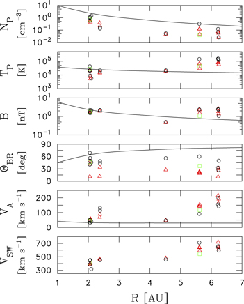
Figure 2. Comparison of plasma conditions during data samples used in this study. Red triangles are values when waves due to either pickup H+ or He+ are observed. Black circles are values during control intervals without waves due to either source. Top to bottom: solar wind thermal proton density, NSW, with solid curve given by  expansion with 6 p+ cm−3 at 1 au; thermal proton temperature, TP, where the solid curve uses
  fit to Voyager data (Richardson et al. 1995a); magnetic field intensity
  , where the solid curve assumes 6 nT at 1 au and evolves according to Parker (1963); angle between the mean magnetic field and the radial direction,
  , where the solid curve assumes Parker evolution from 45° at 1 au; Alfvén speed, where the solid curve assumes the above values.
Download figure:
Standard image High-resolution image3.1. Spectral Analysis
We combine several spectral analysis methods in this paper. Power and magnetic helicity spectra are computed using Blackman–Tukey techniques (Matthaeus & Smith 1981; Smith 1981; Matthaeus & Goldstein 1982; Matthaeus et al. 1982; Leamon et al. 1998b; Smith et al. 2006a, 2006c; Hamilton et al. 2008; Joyce et al. 2010). We show the normalized magnetic helicity  (Matthaeus & Smith 1981; Smith 1981; Matthaeus & Goldstein 1982; Matthaeus et al. 1982), which is the spatial analog of the polarization. Fast Fourier transform techniques are used to compute the polarization parameters (Fowler et al. 1967; Rankin & Kurtz 1970; Means 1972; Mish et al. 1982), as well as power and helicity spectra, which agree with the Blackman–Tukey analyses. Polarization parameters are computed in mean-field coordinates (Belcher & Davis 1971; Bieber et al. 1996). The polarization parameters that we will show are the degree of polarization
  , coherence
  , ellipticity
  , and angle between the minimum variance direction
  and mean magnetic field
  given by
  . We part with the convention of Mish et al. (1982) and place the sign of polarization on the ellipticity instead of the degree of polarization so that
  (
( ) denotes left-hand (right-hand) polarization. For typical solar wind observations where kinetic instabilites are not evident,
  , although many of the background examples shown here do show a marginally elevated level of Dpol and Coh. Fluctuations at dissipation scales that are generally higher in frequency than the waves studied here show
  . For typical wave events at the frequencies modified by the kinetic instability, we find
  while
while  and
and  . The normalized magnetic helicity,
  , will take on values of ±1 according to the direction of the mean magnetic field (Smith et al. 1984).
The time intervals and ambient plasma parameters for data intervals shown in this paper (both wave events and their associated control intervals) are listed in Table 1. The table lists times, spacecraft locations, and ambient plasma conditions along with statements (Yes/No) of whether the interval displays waves in association with newborn interstellar pickup He+ or H+. The two intervals of questionable wave signatures are listed as "??." Most of the data are from rarefaction intervals. The exception to this is V1 on day 51 of 1978, when the spacecraft seems to be within an ejecta region of low density and cold plasma.
Table 1. Data Interval Parameters
| s/c | He+ Waves? | H+ Waves? | Year | Time | R |

|
VSW | NSW | VA |

|
|---|---|---|---|---|---|---|---|---|---|---|
| Yes/No | Yes/No | (AU) | (deg) | (km s
|
(cm−3) | (km s−1) | (mHz) | |||
| V2 | ?? | No | 1978 | 15.38–15.54 | 2.04 | 46.2 ± 2.5 | 414.0 ± 2.1 | 0.720 ± 0.070 | 44.7 | 26.4 |
| V2 | Yes | No | 1978 | 16.04–16.13 | 2.05 | 11.3 | 394.1 | 0.541 | 48.6 | 24.9 |
| V2 | No | No | 1978 | 16.29–16.50 | 2.05 | 49.7 ± 4.8 | 387.2 ± 3.3 | 0.601 ± 0.064 | 51.0 | 27.6 |
| V1 | No | No | 1978 | 14.25–14.50 | 2.05 | 68.7 ± 14.8 | 446.1 ± 8.9 | 1.13 ± 0.26 | 45.6 | 33.8 |
| V1 | No | No | 1978 | 14.50–14.75 | 2.06 | 56.2 ± 1.4 | 451.1 ± 0.8 | 1.01 ± 0.11 | 32.7 | 22.9 |
| V1 | Yes | Yes | 1978 | 15.50–15.75 | 2.07 | 48.5 ± 4.4 | 403.0 ± 1.2 | 0.529 ± 0.024 | 55.5 | 28.1 |
| V1 | Yes | No | 1978 | 16.25–16.50 | 2.07 | 41.6 ± 3.0 | 381.9 ± 1.0 | 0.425 ± 0.012 | 57.8 | 26.3 |
| V1 | No | No | 1978 | 18.75–19.00 | 2.10 | 45.9 ± 6.0 | 319.4 ± 2.0 | 1.44 ± 0.13 | 39.3 | 32.9 |
| V2 | Yes | No | 1978 | 52.04–52.25 | 2.37 | 11.5 ± 3.1 | 469.1 ± 3.4 | 0.39 ± 0.04 | 69.2 | 30.0 |
| V2 | Yes | No | 1978 | 52.48–52.63 | 2.38 | 34.0 ± 11.5 | 455.1 ± 4.1 | 0.22 ± 0.06 | 88.8 | 29.2 |
| V2 | No | No | 1978 | 52.48–52.92 | 2.38 | 43.5 ± 9.2 | 453.5 ± 4.7 | 0.16 ± 0.05 | 114. | 31.8 |
| V2 | No | No | 1978 | 52.71–52.88 | 2.38 | 48.4 ± 5.0 | 452.1 ± 4.9 | 0.13 ± 0.01 | 131. | 33.4 |
| V2 | Yes | Yes | 1979 | 7.81–8.00 | 4.52 | 27.6 ± 1.9 | 480.4 ± 0.9 | 0.045 ± 0.001 | 47.5 | 7.0 |
| V2 | No | No | 1979 | 8.83–9.00 | 4.52 | 55.8 ± 1.4 | 460.8 ± 1.2 | 0.054 ± 0.001 | 46.8 | 7.6 |
| V2 | No | No | 1979 | 264.15–264.35 | 5.61 | 59.7 ± 10.7 | 711.5 ± 10.9 | 0.32 ± 0.04 | 91.4 | 36.1 |
| V2 | Yes | Yes | 1979 | 265.33–265.52 | 5.62 | 22.8 ± 3.6 | 642.1 ± 5.8 | 0.12 ± 0.01 | 145. | 35.3 |
| V2 | Yes | Yes | 1979 | 265.31–265.67 | 5.62 | 21.3 ± 3.7 | 636.9 ± 9.7 | 0.12 ± 0.01 | 143. | 34.6 |
| V2 | Yes | Yes | 1979 | 266.15–266.54 | 5.62 | 18.7 ± 10.4 | 592.8 ± 15.1 | 0.05 ± 0.01 | 155. | 23.4 |
| V2 | ?? | ?? | 1979 | 267.02–267.17 | 5.62 | 37.0 ± 5.5 | 542.2 ± 1.4 | 0.040 ± 0.004 | 117. | 16.2 |
| V1 | No | Yes | 1979 | 265.48–265.75 | 6.22 | 10.6 ± 4.0 | 719.3 ± 2.5 | 0.07 ± 0.01 | 216. | 41.1 |
| V1 | No | No | 1979 | 266.00–266.19 | 6.22 | 32.7 ± 8.2 | 649.1 ± 15.9 | 0.12 ± 0.02 | 155. | 37.4 |
| V1 | No | No | 1979 | 266.75–266.96 | 6.23 | 27.3 ± 9.5 | 659.1 | 0.06 | 200. | 35.5 |
| V1 | Yes | Yes | 1979 | 267.15–267.50 | 6.23 | 30.6 ± 2.5 | 640.9 ± 10.5 | 0.06 ± 0.01 | 166. | 27.6 |
| V1 | Yes | Yes | 1979 | 268.50–268.75 | 6.24 | 25.4 ± 2.1 | 616.4 ± 5.5 | 0.025 ± 0.002 | 191. | 20.9 |
| V1 | No | No | 1979 | 269.50–269.75 | 6.24 | 49.6 ± 10.9 | 595.4 ± 9.9 | 0.026 ± 0.005 | 143. | 16.2 |
Download table as: ASCIITypeset image
Figure 3 shows our analysis of six data intervals that characterize the different types of observations found. The spacecraft and times are given at the top of each stack of magnetic spectra. Each stack of six panels represents a single data interval. The spectra are (top to bottom) total power spectrum (trace of the power spectral density matrix) and the power spectrum of the magnitude  time series, degree of polarization, coherence, ellipticity, angle between the minimum variance direction and mean-field direction, and normalized magnetic helicity as defined above.

Figure 3. Our analysis of six intervals of data with spacecraft and times marked at the top of each stack. Each stack contains (top to bottom) the spectrum of the total power and power in  , degree of polarization, coherence, ellipticity, angle between the minimum variance direction and the mean magnetic field, and the normalized magnetic helicity.
Download figure:
Standard image High-resolution imageThe top left panel of Figure 3 shows a control interval without evidence of waves due to pickup ions. The data were recorded by V2 in 1978 on day 15 from 09:00 to 13:00 UT. The spacecraft is in the same rarefaction interval shown in Figure 1 with only a minimal time shift allowing for the transit time of the wind between V1 and V2. Both the total power and  spectra are power laws with a factor of ∼10 difference between the two, indicating that the fluctuations are transverse to the mean field and largely noncompressive in the sense that compressive fluctuations show larger fluctuations in
  . Dpol, Coh, Elip,
  , and
, and  are all
  , which is typical of the background interplanetary field. This indicates fluctuations that do not maintain coherence over many wavelengths, do not favor one sense of rotation over another, and are transverse to the mean magnetic field.
  is often taken from wave theory to indicate propagation along the mean magnetic field, and this is consistent with certain wave types; however, it is also consistent with 2D turbulence, where the fluctuations are confined to the perpendicular plane and the minimum variance direction is along the mean magnetic field. At frequencies sufficiently higher than
  , the value of
  increases to
  . This appears to mark the onset of dissipation dynamics.
The top middle panel of Figure 3 shows a data interval with strong evidence of waves due to pickup He+. The data were recorded by V2 in 1978 from 01:00 to 03:00 UT on day 16, and the spacecraft is again in the same rarefaction interval. There is a peak in the power at  that extends to
  with an
  behavior in the range
  as predicted by theory (Lee & Ip 1987). The enhanced power extends to
  , but the spectrum falls more steeply than
  in the range
  . The background spectrum appears to be a power law and is given by the dashed line. The spectrum of
  also shows enhanced power in the same range, but is a factor of ∼10 smaller than the total power, again indicating that the fluctuations are largely transverse. Dpol and
  while
while  ,
,  , and
, and  . All of these findings point to parallel-propagating, transverse magnetic waves with left-hand polarization in the spacecraft frame arising from newborn pickup He+. There is some question as to whether some of these waves are due to pickup H+. The wave signatures become less evident for frequencies marginally larger than the cyclotron frequency, and the spectrum follows the
  form that is predicted for a single resonance. For this reason, we suspect that all of the waves are due to the He+ resonance. However, it is difficult to assert that the H+ resonance has not produced significant wave growth that is separable from the He+ signature, and our analyses below indicate that it has. We suggest that when He+-associated waves extend to frequencies greater than
  , these waves can, at times, scatter the pickup H+ toward isotropy without the associated production of H+ spectral signatures. Again, as in most instances,
  at frequencies greater than
  , which appears to mark the onset of dissipation dynamics.
The top right panel of Figure 3 shows our analysis of V1 data from 1978, day 15, hours 12:00 to 18:00 UT. The spacecraft is in the rarefaction interval shown in Figure 1 at a time with a strong He+ instability and undeniable H+ wave signatures. Except for  , the analysis shows a distinct bimodal signature consistent with growth due to both pickup ion populations and weakened wave characteristics between the two. Careful examination indicates that there is no evidence of wave growth at frequencies less than the corresponding cyclotron frequency.
While theory predicts that the wave-associated power spectrum behaves as  (Lee & Ip 1987), this is not always seen here. There can also be a rather abrupt high-frequency cutoff to the polarization signatures. This is seen in spectra above and below. It may suggest an incomplete scattering of the pickup ions, which leads to less than nominal wave growth at the high frequencies (Möbius et al. 1998).
The bottom left panel of Figure 3 shows spectra from V2 in 1978 from 11:30 to 15:00 UT on day 52. There is a weak wave power enhancement associated with the He+ resonance and no evidence of an H+ signature. At this time the spacecraft is not within a rarefaction interval, but the observation comes ∼14 hr after a data gap of ∼12 hr duration when the wind speed increases and the density decreases. There may be a shock at ∼14:00 UT on day 50. There is no evidence of waves between the shock or the data gap and this time period, making it unlikely that the waves originate with a possible shock within the data gap. The density continues to decrease until ∼3 hr after the wave observation, although the wind speed is largely constant. The spacecraft may be within a magnetic cloud (Burlaga et al. 1990; Gosling 1990). The enhanced wave power is low, but the polarization signatures are strong for  and do not extend to
  . This is certainly an interval where the waves are excited only by He+ and not H+.
The bottom middle panel of Figure 3 shows spectra from V2 in 1979 from 08:00 to 12:30 UT on day 265. The spacecraft is again in a rarefaction interval lasting 8 days when the wind speed falls from 1000 to 500 km s−1 and the density falls from nearly 1 p+ cm−3 to under 0.01 p+ cm−3. There is strong evidence of an H+ resonance with the wave signatures extending back to  . For this reason we contend that there are waves present due to the He+ resonance and the H+ resonance.
The bottom right panel of Figure 3 shows spectra from V1 in 1979 from 12:00 to 18:00 UT on day 268. The spacecraft is within a rarefaction interval, and there may be a shock within a data gap 6 days earlier. There is no evidence of shock-associated waves between the shock passage and this wave interval. There is clear evidence of both an He+ and H+ resonance. The two signatures are separate and distinct. The form of the power spectrum does approximate the  predicted by Lee & Ip (1987) for each of the wave power enhancements. It is likely that the resolution of two separate enhancements is attributable to the low level of the enhanced power, which allows the He+ waves to fade into the background spectrum before the onset of the H+ resonance.
We average the polarization spectra Dpol, Coh, Elip, and  over the range
  for all time periods listed in Table 1. Figure 4 shows the result of that analysis, where red triangles represent intervals with enhanced wave activity due to He+ and black circles represent intervals without waves attributed to He+. Green squares mark the two intervals where the presence of waves due to He+ is questionable. Note that Dpol and Coh values are consistently greater when waves are present than when they are not. Values of Elip are consistently more negative for wave events, while non-wave events show values
  . The two intervals where the wave-like attributes of the spectra are questionable appear to be much more like background events than wave events in these plots. The minimum variance direction given by
  is a less effective determinant of wave activity, with both wave events and control intervals showing
  .
.
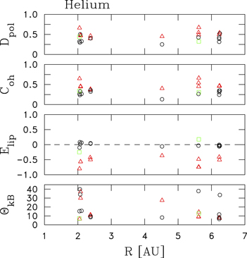
Figure 4. Polarization characteristics for wave intervals (red triangles) and control intervals (black circles) for  for the intervals listed in Table 1. Green squares mark an interval when the presence of waves is uncertain. Top to bottom: degree of polarization, coherence, ellipticity, and angle between the minimum variance direction
  and mean magnetic field direction. All parameters are plotted as a function of heliocentric distance.
Download figure:
Standard image High-resolution imageFigure 5 shows our analysis of the polarization associated with the H+ resonance, averaging the parameters over the range  . The conclusions, except for the polarization of the one event described below, are the same as with the He+ resonance. The waves tend to have Dpol and Coh higher than events without waves. The waves have
  except for the one event described in the next paragraph and
  . Except for
  , the wave events show polarization parameters that are distinct from non-wave events. Again, the one event with questionable spectra appears more like a control interval than a wave interval.
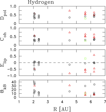
Figure 5. Same as Figure 4, but for frequencies  .
.
Download figure:
Standard image High-resolution imageFigure 6 shows our analysis of V1 data for the one case that is exceptional owing to the measured polarization of the waves. This is a V1 observation in 1979 from day 265.48 to 265.75. There is no evidence of wave generation by pickup He+ in this event. The spectrum of  demonstrates an unfortunate aspect of the Blackman–Tukey method, where undersampled or poorly sampled frequencies can exhibit negative power and the offending frequencies are omitted from the plot. This is not a problem here since the anomalous behavior is limited to the lowest frequencies and the spectrum still resolves
  . The Dpol and Coh spectra, along with
  , all point to wave activity for
  . The Elip and
  spectra are consistent with right-hand polarized waves in the spacecraft frame. This is not what is expected, but ∼10% of the events studied by Cannon et al. (2014a, 2014b) exhibited this same unexpected behavior. We include this event in our analysis even though it is not fully understood.
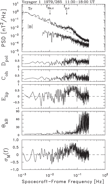
Figure 6. Format same as Figure 3 showing the spectra of the one wave event associated with the H+ resonance showing an unexpected right-hand polarization in the spacecraft frame. In all other regards, this appears to be an observation of waves due to pickup H+.
Download figure:
Standard image High-resolution imageTwo of the spectra shown in Figure 3 have overlapping analyses listed in Table 1. The first such instance is seen in the bottom left panel of Figure 3 and corresponds to V2 observations in 1978 from day 52.48 to 52.63 (11:30–15:00 UT). The overlapping analysis interval (not shown) extends from day 52.48 to 52.92 (11:30–22:00). There is no clear evidence of waves in this second analysis, which demonstrates that the wave signal, which is presumably during the earlier part of the overlapping time interval, is diluted by the later data. Efforts to compute spectra for significantly shorter data intervals result in poor spectral estimates. We do not guarantee that we have found all of the waves due to newborn interstellar pickup ions in the years of data studied.
The second such instance is seen in the bottom middle panel of Figure 3 and corresponds to V2 observations in 1979 from day 265.33 to 265.52 (8:00–12:30 UT). The overlapping analysis interval extends from day 265.31 to 265.67 (7:30–16:00 UT). The wave signatures in this second interval are present, but again reduced, indicating how brief the wave intervals can be. In both instances, but more prominantly in the former, the wave power for  is consistent with the formation of the anticipated
  spectrum associated with the He+ resonance. This feature appears to be absent from the H+ resonance.
3.2. Theory Application
Having established a list of events, we now apply the theories for wave excitation and turbulent cascade to the observations. The power levels for the spectral peaks are obtained from the analysis. The values for the background spectra at the corresponding cyclotron frequency are obtained by extrapolation of the power-law background at lower and higher frequencies. Mean plasma parameters (VSW, VA, NSW, etc.) are obtained by averaging the hourly Voyager observations over the prescribed time. In some instances, there are too few data to obtain an uncertainty for some parameters.
Figure 7 shows He ionization parameters for the time periods of Table 1. The top panel shows  , the ionization rate that depends solely on solar UV radiation. The second panel shows the He+ production rate, which is the product of
  and the neutral He density. We take the neutral He density to be a constant at these radial distances. Both of these rates follow a simple
  dependence, and there is no difference between wave and non-wave events. The dashed lines in the top two panels give the
  behavior expected for the variables. The bottom panel shows the rate of wave energy excitation as computed from Equation (4). Contrary to the production of He+, the wave energy excitation rate,
  , increases with distance from the Sun. There is no consistent or significant difference between wave energy excitation in wave and non-wave events. This suggests that the observability of waves does not depend on the rate of wave excitation alone.
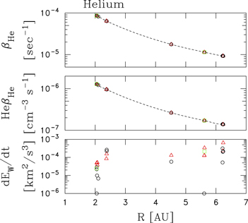
Figure 7. Top to bottom: rate of He ionization  for wave events (red triangles) and control events (black circles), as well as two unknown intervals (green squares). Computed He+ production rate He
 and rate of wave energy production as computed from Equation (4).
Download figure:
Standard image High-resolution imageFigure 8 shows some of the key parameters involved in the excitation of wave energy by H+. Charge exchange is a component of H+ production, so we plot the flux of thermal protons in the solar wind, FSW. The flux decreases nominally as NSW, which varies as  , but rarefaction regions represent lower densities and average wind speeds, making the thermal ion flux low in these intervals. Still,
  for the intervals studied. The density of neutral H increases with distance from the Sun, while the ionization rate
  decreases. The resulting H+ production rate
  is nearly constant, but decreases precipitously inside 2 au owing to the exponential reduction in neutral H. The resultant excitation rate for wave energy,
  , increases with distance from the Sun. In the case of H+ resonance, the rate of wave energy excitation in wave events does appear to be marginally greater than in data intervals not exhibiting wave activity, although there are exceptions to that statement, as seen in the figure.
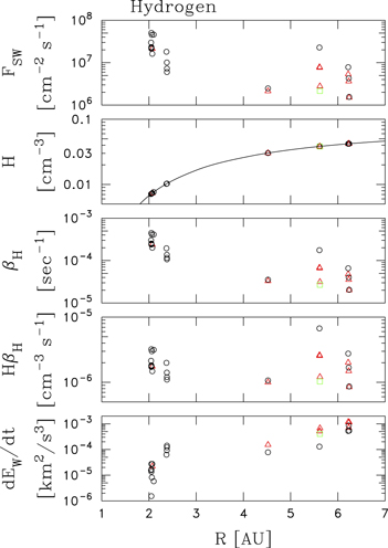
Figure 8. Parameters associated with the excitation of waves due to H+. Top to bottom: flux of solar wind protons, neutral H density, H ionization rate, H+ production rate, and wave excitation rate due to the generation of H+.
Download figure:
Standard image High-resolution imageFigure 9 compares the background power spectrum level, Pback, at  and
and  for wave and non-wave events. Low background power levels make it easier for a prescribed amount of wave energy to be observable. While there is a strong tendency for wave events to have lower background levels, there are exceptions. The background power spectrum,
  , for these short intervals is very much the result of local flow conditions. Also, we have already shown that the magnetic field is generally more radial than the Parker field model would predict (Parker 1958, 1963). This is consistent with the observation that the rarefaction regions are of the type described by Gosling & Skoug (2002) and Schwadron (2002).
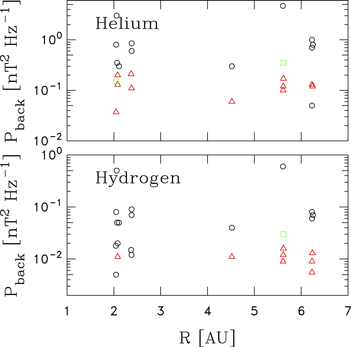
Figure 9. Plot of the spectral power in the background spectrum at both the He+ (top) and H+ (bottom) cyclotron frequencies. Red triangles, black circles, and green squares continue the same designation as above. It is true that the background spectum tends to be lower during wave events than for adjacent controls, although the correlation is not perfect. This could indicate that waves are seen when the given excitation rate raises the wave power above the background, or it may also suggest that the weaker turbulence that is associated with lower power levels permits the weak instability to accumulate sufficient energy as to become observable.
Download figure:
Standard image High-resolution imageFigure 10 shows the time required for Equation (4) to achieve the observed wave power. For control events the plot shows the time required to achieve the background power level. However, there is no assertion that the wave power at these times is as great as the background level. Two computed times for wave growth due to He+ are off the scale and represented by arrows at the top of the panel. It is evident that the 20–40 hr estimates used to compute the rate of wave energy growth are generally a good approximation. There are intervals requiring more time to achieve the observed wave power, but the growth rate is linear so that rates obtained using the 20–40 hr estimates remain valid. Accumulation times like these represent solar wind transit times for 0.3–1 au, suggesting that the multiple au accumulation times of Lee & Ip (1987) are unlikely. Whether this is the result of the interruption of the instability at some point in time or the gradual erosion of wave energy by the turbulence while the instability is active, wave power levels are not consistent with the accumulation of wave energy over many au.

Figure 10. Excitation time for wave generation using Equation (4) and ion production rates to determine wave energy equal to the individual observation.
Download figure:
Standard image High-resolution imageCannon et al. (2014b) demonstrated that the determining factor in the observability of waves due to newborn interstellar H+ is low turbulent cascade rates as computed from Equation (6) when compared to wave growth rates as computed from Equation (4). Figure 11 reproduces that analysis using the waves found in this study. Wave events consistently show growth rates that exceed the turbulent cascade rate. The non-wave observations are less consistent in that there are a minority of background events showing weak turbulence conditions that favor wave growth despite the fact that waves are not seen during these intervals. Recent studies of the turbulent cascade at 1 au have shown that the turbulent cascade can be highly variable in the sense of intermittency relative to the mean predicted by Equation (6) (Coburn et al. 2014, 2015).

Figure 11. Comparison of wave energy production rates to the predicted rate of energy transfer due to turbulence. Waves are seen when excitation rates exceed turbulence rates.
Download figure:
Standard image High-resolution image
4. DISCUSSION
It is desirable to measure the cross-correlation between the magnetic and solar wind velocity fluctuations, the "cross-helicity," from which the wave propagation directions can be inferred. This was performed by Joyce et al. (2010). The He+ waves seen by V2 on DOY 7 and 8 of 1979, again studied here, were determined to be propagating sunward. Joyce et al. (2010) show that the Nyquist frequency for the cross-helicity spectra,  , is ∼5 mHz, where δ is the time resolution of the particle data from the PLS instrument on Voyager. Comparison of
  for the various events shows that the Joyce et al. event has a considerably smaller
  than all other events. Computing
  from the values of
  listed, only three data intervals other than that studied by Joyce et al. have
  , and those are marginal at ∼4 mHz. Thus, it is not possible to determine reliable values of the cross-helicity, and from that infer the propagation direction of the waves, for any events shown here except the Joyce et al. event that has already been studied.
The rate of wave energy production increases with distance from the Sun at least insofar as this limited ensemble of events would indicate. Wave growth as a result of H+ is  greater at 6 au than at 2 au, which is, in part, due to the exponential rise in neutral H in this region of interplanetary space. Wave growth due to He+ increases by only ∼10 over this same range. The typical thermal proton temperature decreases out to 20 au and then begins to increase slowly beyond that distance as the plasma continues to expand (Matthaeus et al. 1994; Richardson et al. 1995b, 1996; Zank et al. 1996, 2012; Smith et al. 2001, 2006b; Isenberg et al. 2003, 2010; Richardson & Smith 2003; Breech et al. 2005, 2008, 2009, 2010; Ng et al. 2010; Oughton et al. 2011). A careful statistical analysis involving more events and data from greater heliocentric distance would be required to determine whether waves due to newborn interstellar pickup ions are more or less likely beyond 6 au. That study is beyond the scope of this effort, as the requiste data beyond 6.25 au are currently unavailable.
We have used a rather simple scaling of the turbulent cascade rate to represent the diverse nonlinear processes that disperse coherent wave energy in interplanetary space. The general subject of MHD turbulence remains relatively young with many unanswered questions. The related questions of dynamics, geometry, rates, and the role of waves in the nonlinear dynamics are only partially explored. Even the general state of the turbulence in the outer heliosphere is at best partially understood. Therefore, the use of Equation (6) to describe the turbulence should be viewed as preliminary and illustrative.
It is unlikely that these observations are related to the low-frequency wave (LFW) storm observations of Jian et al. (2010, 2014) and Boardsen et al. (2015). Those waves, which have been seen at and inside 1 au, are seen at frequencies  and with mixed polarization. Jian et al. (2014) argue credibly that LFW storm events are not related to newborn interstellar or cometary pickup ions.
Future studies of this type involving waves in the more distant heliosphere and heliosheath may be required to consider wave dispersion effects due to the accumulated presence of interstellar pickup ions (Zank et al. 2014). However, the density of this suprathermal component is relatively low at the heliocentric distances examined here, and this added complication has been omitted from this analysis.
5. SUMMARY
We have studied the Voyager magnetic field data from day 329 of 1977 to day 288 of 1979 and found further examples of waves excited by newborn interstellar pickup H+ and He+. Based on recent reports of waves due to interstellar H+ observed by the Ulysses spacecraft (Cannon et al. 2014a, 2014b), we focused our search on rarefaction regions and other intervals of unusally low magnetic fluctuation levels. We found examples of waves at frequencies greater than the corresponding cyclotron frequency with left-hand polarization in the spacecraft frame and high degrees of polarization and coherence. We found one event with unexpected right-hand polarization in the spacecraft frame, which is consistent with a minority of events found by Cannon et al. (2014a). All other aspects of the measurement were consistent with expectations.
There are no direct observations of pickup ions from instruments on the Voyager spacecraft, so we are required to estimate ion production based on theory. We have assumed that the neutral He is constant everywhere in the region of study, that He+ production is via photoionization, and that the ionization efficiency varies as the inverse square of the heliospheric distance. Neutral H is assumed to vary according to theory with an exponential decrease in density inside ∼5 au (Zank 1999). We used the average solar luminosity in the UV range as with He ionization and added ionization rates due to charge exchange with thermal protons. Any possible variation in solar UV luminosity was not taken into account.
We have compared wave growth rates due to pickup ions to the rate at which turbulence disperses the energy as part of the nonlinear cascade. For observed wave intervals, the growth rate of wave energy due to pickup ions exceeds the rate of turbulent cascade that destroys coherent structures. For intervals without observable wave activity, the comparison is mixed, but turbulence rates generally exceed wave growth rates, preventing the spectral accumulation of wave energy over long periods of time.
These findings continue to be consistent with the premise that newly ionized interstellar pickup ions are unstable to generating quasi-parallel-propagating transverse electromagnetic waves (i.e., fast mode and ion-cyclotron mode) wherever they appear in the solar wind. These waves may not be observable when turbulent interactions dominate the wave growth, but the fluctuation energy created by the pickup ion isotropization is still added to the turbulent cascade under these conditions. This additional turbulent energy is responsible for the increasing temperature of the core solar wind, as measured by Voyager 2 inside the termination shock. These conclusions should also have important implications for the fate of secondary pickup ions in the outer heliosheath, potentially acting as source particles for the IBEX ribbon (Heerikhuisen et al. 2010; Möbius et al. 2013; Schwadron & McComas 2013; Isenberg 2014).
C.W.S. is supported by Caltech subcontract 44A1085631 to the University of New Hampshire in support of the ACE/MAG instrument. Part of the ACE mandate is to better understand the role of pickup ions in the heliosphere. P.A.I. is supported by NASA grants NNX13AF97G and NNX11AJ37G, as well as NSF grant AGS0962506. B.J.V. is supported by NSF grant AGS1357893. P.A. and D.K.T. were undergraduate summer researchers at UNH at the time this work was performed. C.J.J. is a graduate student in the Physics program at UNH, whose earlier work initiated this line of investigation.