Systematic Review of Decision Making Algorithms in Extended Neutrosophic Sets

Abstract

The Neutrosophic set (NS) has grasped concentration by its ability for handling indeterminate, uncertain, incomplete, and inconsistent information encountered in daily life. Recently, there have been various extensions of the NS, such as single valued neutrosophic sets (SVNSs), Interval neutrosophic sets (INSs), bipolar neutrosophic sets (BNSs), Refined Neutrosophic Sets (RNSs), and triangular fuzzy number neutrosophic set (TFNNs). This paper contains an extended overview of the concept of NS as well as several instances and extensions of this model that have been introduced in the last decade, and have had a significant impact in literature. Theoretical and mathematical properties of NS and their counterparts are discussed in this paper as well. Neutrosophic-set-driven decision making algorithms are also overviewed in detail.

1. Introduction

The Neutrosophic set (NS) originates from neutrosophy, which is a branch of philosophy that provides a means to imitate the possibility and neutralities that refer to the grey area between the affirmative and the negative common to most real-life situations [1]. Let <M> be an element, which can be an idea, an element, a proposition, or a theorem, etc.; with <anti M> being the opposite of <M>; while <neut M> is neither <M> nor <anti M> but is the neutral linked to <M>; e.g., <M> = success, <anti M> = loss, and <neut M> = tie game. Another example to understand this concept is to let <M> = voting for a candidate, we would have <anti M> = voting against, and<neut M> = blank vote. If <anti M> does not exist, {m<anti M> = 0}. Similarly, if <neut M> does not exist, {m<neut M> = 0} [1]. This type of issue is an example of a Fuzzy Set (FS) and Intuitionistic Fuzzy Set (IFS) that can be handled by a NS with indeterminacy membership [2,3]. Therefore, for addressing many decision making problems that involve human knowledge, which is often pervaded with uncertainty, indeterminacy, and inconsistency in information, the concept of NS can be useful. Areas such as artificial intelligence, applied physics, image processing, social science, and topology also suffer from the same problems.

On the basis of the FS and its extended concepts (interval valued FS, intuitionistic FS, and so on), by accumulation an independent indeterminacy association function to the existing IFs model proposed by Atanassov [2], Smarandache [3] proposed the concept of NS. Several extensions and special cases of NSs have been proposed in the literature. These cases include the single valued neutrosophic sets (SVNS) [3,4], interval neutrosophic sets (INs) [5], Neutrosophic Soft Set (NSS) [6], INSS [7], Refined Neutrosophic Set (RNS) [8], INRS [9], IVNSRS [10], CNS [11], bipolar neutrosophic sets (BNS) [12], and neutrosophic cube set [13]. Recently, NSs have become a fascinating research topic and have drawn wide attention. Some of the most significant developments in the study of NS include the introduction of SVNSs and INSs. Wang et al. [14] suggested a SVNS to accommodate engineering and scientific problems. The authorsalso proposed INSs in which association, indeterminacy, and non-association are extended to interval numbers [15]. The SVNS and INS models are the most renowned and most ordinarily used among the neutrosophic models in literature. Many different characteristics of these models have been studied in the literature. These include decision making methods, correlation coefficients, information measures and optimization techniques.

In the extent of natural science, operations research, economics, management science, military affairs, and urban planning, NSs have a broad application. They also can be applied todecision making problems when the ambiguity and complexity of the attributes make the problems impossible to be expressed or valued with real numbers. There were some studies of multi-criteria decision-making methods based on SVNS [16,17,18,19,20,21,22,23,24,25,26,27], INs [28,29,30,31,32,33,34,35], BNs [36,37,38], generalized neutrosophic soft set [39,40], neutrosophic refined set [41,42,43,44], and triangular fuzzy neutrosophic number set (TFNNs) [45,46,47,48,49]. This paper presents an overview of NSs and some of the most significant instances and extensions of NS, as well as the application of these models in multiple attribute decision-making (MADM) problems. The neutrosophic models that will be reviewed in this paper include theSVNS [14], INS [15], BNS [12], ReNS [31], and the aggregation of TFNS [47].The neutrosophic set has been also applied to various applications [50] such as e-learning [51], medical image denoising [52], Strogatz’s spirit [53].

Section 2 presents an overview of NS that includes its background and the origin of the concept, the formal definition of neutrosophic sets, and the motivation behind the introduction of neutrosophic sets. Section 3 presents an overview of several instances and extensions of neutrosophic sets including the definition and properties while Section 4 presents decision making approaches for these models. Section 5 presents the concluding remarks, followed by the acknowledgements and the list of references.

2. Preliminary

Definition 1

([1]).Let a space of discourse be$U$with a general element$\stackrel{⃛}{h}\in U$. A NS$\stackrel{⃛}{Y}$in$U$is described by a truth-association function$t_{\stackrel{⃛}{Y}},$an indeterminacy-association function$i_{\stackrel{⃛}{Y}}$and a non-association function$f_{\stackrel{⃛}{Y}},$where$t_{\stackrel{⃛}{Y}}\left(\stackrel{⃛}{h}\right), i_{\stackrel{⃛}{Y}}\left(\stackrel{⃛}{h}\right), f_{\stackrel{⃛}{Y}}\left(\stackrel{⃛}{h}\right)$, are real standard or non-standard subsets of$\left]{}^{-}0, 1^{+}\right[$so that$t_{\stackrel{⃛}{Y}}:U\to \left]{}^{-}0, 1^{+}\right[ ,i_{\stackrel{⃛}{Y}}:U\to \left]{}^{-}0, 1^{+}\right[,f_{\stackrel{⃛}{Y}}:U\to \left]{}^{-}0, 1^{+}\right[.$The sum of three independent association degrees$t_{\stackrel{⃛}{Y}}\left(\stackrel{⃛}{h}\right), i_{\stackrel{⃛}{Y}}\left(\stackrel{⃛}{h}\right), f_{\stackrel{⃛}{Y}}\left(\stackrel{⃛}{h}\right)$, satisfies the following condition/constraint:

$$0^{-}\le \sup t_{\stackrel{⃛}{Y}}\left(\stackrel{⃛}{h}\right)+\sup i_{\stackrel{⃛}{Y}}\left(\stackrel{⃛}{h}\right)+\sup f_{\stackrel{⃛}{Y}}\left(\stackrel{⃛}{h}\right)\le 3^{+}$$

Definition 2

([14]).Let a space of discourse be$U$with a general element$\stackrel{⃛}{h}\in U$. A SVNS$\stackrel{⃛}{M}$in$U$is categorized by a truth association function$t_{\stackrel{⃛}{M}}$, indeterminacy association function$i_{\stackrel{⃛}{M}}$and non-association function$f_{\stackrel{⃛}{M}}$such that for each point$\stackrel{⃛}{h}\in U$,$t_{\stackrel{⃛}{M}}\left(\stackrel{⃛}{h}\right), i_{\stackrel{⃛}{M}}\left(\stackrel{⃛}{h}\right), f_{\stackrel{⃛}{M}}\left(\stackrel{⃛}{h}\right)\in \left[0, 1\right],$i.e., their cardinality is 1. When$U$is continuous, a SVNS$\stackrel{⃛}{M}$can be stated as:

$$\stackrel{⃛}{M}={\displaystyle \underset{U}{\int }\frac{\langle t_{\stackrel{⃛}{M}}\left(\stackrel{⃛}{h}\right), i_{\stackrel{⃛}{M}}\left(\stackrel{⃛}{h}\right), f_{\stackrel{⃛}{M}}\left(\stackrel{⃛}{h}\right)\rangle }{\stackrel{⃛}{h}},\stackrel{⃛}{h}\in U.}$$

When$U$is discrete, a SVNS$\stackrel{⃛}{M}$can be stated as:

$$\stackrel{⃛}{M}={\displaystyle \sum _{i=1}^n\frac{\langle t\left(\stackrel{⃛}{h}\right), i\left(\stackrel{⃛}{h}\right), f\left(\stackrel{⃛}{h}\right)\rangle }{{\stackrel{⃛}{h}}_i},{\stackrel{⃛}{h}}_i\in U.}$$

Definition 3

([5]).Let a space of discourse be$U$with a general element$\stackrel{⃛}{h}\in U$. An INS$\stackrel{⃛}{M}$in$U$is defined as:$\stackrel{⃛}{M}=\left\{\stackrel{⃛}{h}\left(t_{\stackrel{⃛}{M}}\left(\stackrel{⃛}{h}\right), i_{\stackrel{⃛}{M}}\left(\stackrel{⃛}{h}\right), f_{\stackrel{⃛}{M}}\left(\stackrel{⃛}{h}\right)\right)|\stackrel{⃛}{h}\in U\right\}$, where$t_{\stackrel{⃛}{M}}$,$i_{\stackrel{⃛}{M}}$and$f_{\stackrel{⃛}{M}}$are the truth interval association function, indeterminacy interval association function, and the non interval association function, respectively. For each point$\stackrel{⃛}{h}$in$U$, we have interval values$f_{\stackrel{⃛}{M}}\left(\stackrel{⃛}{h}\right), i_{\stackrel{⃛}{M}}\left(\stackrel{⃛}{h}\right), f_{\stackrel{⃛}{M}}\left(\stackrel{⃛}{h}\right)\subseteq \left[0, 1\right]$, and$0\le \sup \left(t_{\stackrel{⃛}{M}}\left(\stackrel{⃛}{h}\right)\right)+\sup \left(i_{\stackrel{⃛}{M}}\left(\stackrel{⃛}{h}\right)\right)+\sup \left(f_{\stackrel{⃛}{M}}\left(\stackrel{⃛}{h}\right)\right)\le 3.$

For closeness, the following notation is used to represent an interval neutrosophic value (INV):

$$\stackrel{⃛}{h}=\left(\left[t^{\stackrel{⃛}{L}},t^{\stackrel{⃛}{U}}\right],\left[i^{\stackrel{⃛}{L}},i^{\stackrel{⃛}{U}}\right],\left[f^{\stackrel{⃛}{L}},f^{\stackrel{⃛}{U}}\right]\right).$$

Definition 4

([12]).Let a space of discourse be$U$, then a BNS$\stackrel{⃛}{M}$in$U$is defined as follows:$\stackrel{⃛}{M}=\left\{\stackrel{⃛}{h},\langle t_{\stackrel{⃛}{M}}^{+}\left(\stackrel{⃛}{h}\right),i_{\stackrel{⃛}{M}}^{+}\left(\stackrel{⃛}{h}\right),f_{\stackrel{⃛}{M}}^{+}\left(\stackrel{⃛}{h}\right),t_{\stackrel{⃛}{M}}^{-}\left(\stackrel{⃛}{h}\right),i_{\stackrel{⃛}{M}}^{-}\left(\stackrel{⃛}{h}\right),f_{\stackrel{⃛}{M}}^{-}\left(\stackrel{⃛}{h}\right)\rangle |\stackrel{⃛}{h}\in U\right\}$where,

$$t_{\stackrel{⃛}{M}}^{+}\left(\stackrel{⃛}{h}\right),i_{\stackrel{⃛}{M}}^{+}\left(\stackrel{⃛}{h}\right),f_{\stackrel{⃛}{M}}^{+}\left(\stackrel{⃛}{h}\right):U\to \left[0, 1\right]$$

$$t_{\stackrel{⃛}{M}}^{-}\left(\stackrel{⃛}{h}\right),i_{\stackrel{⃛}{M}}^{-}\left(\stackrel{⃛}{h}\right),f_{\stackrel{⃛}{M}}^{-}\left(\stackrel{⃛}{h}\right):U\to \left[-1, 0\right]$$

Analogous to a BNS$\stackrel{⃛}{M}$, the positive association degrees$t_{\stackrel{⃛}{M}}^{+}\left(\stackrel{⃛}{h}\right),i_{\stackrel{⃛}{M}}^{+}\left(\stackrel{⃛}{h}\right)$ and $f_{\stackrel{⃛}{M}}^{+}\left(\stackrel{⃛}{h}\right)$ represent the truth-association, indeterminate association, and non-association of an element $\stackrel{⃛}{h}\in U,$ whereas the negative association degrees $t_{\stackrel{⃛}{M}}^{-}\left(\stackrel{⃛}{h}\right),i_{\stackrel{⃛}{M}}^{-}\left(\stackrel{⃛}{h}\right)$ and $f_{\stackrel{⃛}{M}}^{-}\left(\stackrel{⃛}{h}\right)$ represent thetruth-association, indeterminate association, and non-association of the implicit counter-property of set $\stackrel{⃛}{M}$. For closeness, a BNS is denoted as $\stackrel{⃛}{r}{}_{pq}=\langle t_{pq}^{+}, i_{pq}^{+}, f_{pq}^{+}, t_{pq}^{-}, i_{pq}^{-}, f_{pq}^{-}\rangle .$

Definition 5

([6]).Let a preliminary space set be$U$and$\stackrel{⃛}{M}\subset \stackrel{⃛}{T}$be a set of constraints.Let the set of all neutrosophic subsets of$U$were denoted by$NS(U)$. The collection$(L,\stackrel{⃛}{M})$is named as the NSS over$U$, where$L$is a mapping given by$L:\stackrel{⃛}{M}\to NS(U).$

Definition 6

([6]).Let a preliminary space set be$U$and$\stackrel{⃛}{M}\subset \stackrel{⃛}{T}$be a set of constraints. Let the set of all IN subsets of$U$were denoted by INS. The collection$(L,\stackrel{⃛}{M})$is named to be the INSS over$U$, where$L$is a mapping given by$L:\stackrel{⃛}{M}\to NS(U).$

Definition 7

([6]).Let a preliminary space set be$U$and$\stackrel{⃛}{M}\subset \stackrel{⃛}{T}$be a set of constraints. Let$NS\left(U\right)$be the set of all neutrosophic subsets of$U$. A GNSS$L^{\tilde{\mu }}$over$U$is defined by the set of ordered pairs.

$$L^{\tilde{\mu }}=\left\{\left(L\left(\stackrel{⃛}{s}\right),\tilde{\mu }\left(\stackrel{⃛}{s}\right)\right):\stackrel{⃛}{s}\in \stackrel{⃛}{M},L(\stackrel{⃛}{s})\in \stackrel{⌣}{N}(U),\tilde{\mu }\left(\stackrel{⃛}{s}\right)\in \left[0, 1\right]\right\}$$

(7)

where$L$is a mapping given by$L:\stackrel{⃛}{M}\to N\mathrm{S}(U)\times P$and$\tilde{\mu }$is a fuzzy set such that$\tilde{\mu }:\stackrel{⃛}{M}\to P=\left[0, 1\right].$Here,$L^{\tilde{\mu }}$is a mapping defined by$L^{\tilde{\mu }}:\stackrel{⃛}{M}\to NS(U)\times P.$

For any parameter$\stackrel{⃛}{s}$,$\stackrel{⃛}{h}\in \stackrel{⃛}{M},L(\stackrel{⃛}{h})$is referred to as the neutrosophic value set of parameter$\stackrel{⃛}{s}$, i.e.,$L(\stackrel{⃛}{s})=\left\{\langle \stackrel{⃛}{h},t_{L(\stackrel{⃛}{s})}(\stackrel{⃛}{h}),i_{L(\stackrel{⃛}{s})}(\stackrel{⃛}{h}),f_{L(\stackrel{⃛}{s})}(\stackrel{⃛}{h})\rangle :\stackrel{⃛}{h}\in U\right\}$, where$t,i,f:U\to \left[0, 1\right]$are the associations functions of truth, indeterminacy, and falsity respectively, of the element$\stackrel{⃛}{h}\in U$. For any$\stackrel{⃛}{h}\in U$and$\stackrel{⃛}{s}\in \stackrel{⃛}{M}$,$0\le t_{L(\stackrel{⃛}{s})}(\stackrel{⃛}{h})+i_{L(\stackrel{⃛}{s})}(\stackrel{⃛}{h})+f_{L(\stackrel{⃛}{s})}(\stackrel{⃛}{h})\le 3$.$L^{\tilde{\mu }}$can be stated by:

$$L^{\tilde{\mu }}(\stackrel{⃛}{h})=\left\{\left(\frac{{\stackrel{⃛}{h}}_1}{L(\stackrel{⃛}{s})({\stackrel{⃛}{h}}_1)},\frac{{\stackrel{⃛}{h}}_2}{L(\stackrel{⃛}{s})({\stackrel{⃛}{h}}_2)},\dots ,\frac{{\stackrel{⃛}{h}}_n}{L(\stackrel{⃛}{s})({\stackrel{⃛}{h}}_n)}\right),\tilde{\mu }(\stackrel{⃛}{s})\right\}.$$

Definition 8

([40]).Let a preliminary space set be$U$and$\stackrel{⃛}{M}\subset \stackrel{⃛}{T}$be a set of constraints. Suppose that$INS(U)$is the set of all INSs over$U$defined over$P$, where$P$is the set of all closed subsets of$\left[0, 1\right]$. A GINSS$L^{\tilde{\mu }}$over$U$is defined by the set of ordered pairs of the form.

$$L^{\tilde{\mu }}=\left\{\left(L\left(\stackrel{⃛}{s}\right),\tilde{\mu }\left(\stackrel{⃛}{s}\right)\right):\stackrel{⃛}{s}\in \stackrel{⃛}{M},L(\stackrel{⃛}{s})\in INS(U),\tilde{\mu }\left(\stackrel{⃛}{s}\right)\in \left[0, 1\right]\right\}$$

where$L$is a mapping function given by$L:\stackrel{⃛}{M}\to INS(U)\times P$and$\tilde{\mu }$is a fuzzy set such that$\tilde{\mu }:\stackrel{⃛}{M}\to P=\left[0, 1\right].$Here,$L^{\tilde{\mu }}$is a mapping defined by$L^{\tilde{\mu }}:\stackrel{⃛}{M}\to NS(U)\times P$.

For any parameter$\stackrel{⃛}{s}$,$\stackrel{⃛}{s}\in \stackrel{⃛}{M},L(\stackrel{⃛}{s})$is mentioned to as the interval neutrosophic value set of parameter$\stackrel{⃛}{s}$, i.e.,$L(\stackrel{⃛}{s})=\left\{\langle \stackrel{⃛}{h},t_{L(\stackrel{⃛}{s})}(\stackrel{⃛}{h}),i_{L(\stackrel{⃛}{s})}(\stackrel{⃛}{h}),f_{L(\stackrel{⃛}{s})}(\stackrel{⃛}{h})\rangle :\stackrel{⃛}{h}\in U\right\}$,

$$t_{L(\stackrel{⃛}{s})}(\stackrel{⃛}{h}),i_{L(\stackrel{⃛}{s})}(\stackrel{⃛}{h}),t_{L(\stackrel{⃛}{s})}(\stackrel{⃛}{h}):U\to \mathrm{int}\left[0, 1\right].$$

with the condition

$$0\le \sup t_{L(\stackrel{⃛}{s})}(\stackrel{⃛}{h})+\sup i_{L(\stackrel{⃛}{s})}(\stackrel{⃛}{h})+\sup f_{L(\stackrel{⃛}{s})}(\stackrel{⃛}{h})\le 3,\forall \stackrel{⃛}{h}\in U.$$

The intervals$t_{L(\stackrel{⃛}{s})}(\stackrel{⃛}{h}),i_{L(\stackrel{⃛}{s})}(\stackrel{⃛}{h})$, and$f_{L(\stackrel{⃛}{s})}(\stackrel{⃛}{h})$are the interval-based membership functions for the truth, indeterminacy and falsity for each$\stackrel{⃛}{h}\in U$, respectively. For convenience, let us denote

$$\begin{array}{l}{t}_{L(\stackrel{⃛}{s})}(\stackrel{⃛}{h})=\left[t_{L(\stackrel{⃛}{s})}{}^{\stackrel{⃛}{L}}(\stackrel{⃛}{h}),t_{L(\stackrel{⃛}{s})}{}^{\stackrel{⃛}{U}}(\stackrel{⃛}{h})\right]\\ i_{L(\stackrel{⃛}{s})}(\stackrel{⃛}{h})=\left[i_{L(\stackrel{⃛}{s})}{}^{\stackrel{⃛}{L}}(\stackrel{⃛}{h}),i_{L(\stackrel{⃛}{s})}{}^{\stackrel{⃛}{U}}(\stackrel{⃛}{h})\right]\\ f_{L(\stackrel{⃛}{s})}(\stackrel{⃛}{h})=\left[f_{L(\stackrel{⃛}{s})}{}^{\stackrel{⃛}{L}}(\stackrel{⃛}{h}),f_{L(\stackrel{⃛}{s})}{}^{\stackrel{⃛}{U}}(\stackrel{⃛}{h})\right]\end{array}$$

then$L(\stackrel{⃛}{s})=\left\{\langle \stackrel{⃛}{h},\left[t_{L(\stackrel{⃛}{s})}{}^{\stackrel{⃛}{L}}(\stackrel{⃛}{h}),t_{L(\stackrel{⃛}{s})}{}^{\stackrel{⃛}{U}}(\stackrel{⃛}{h})\right],\left[i_{L(\stackrel{⃛}{s})}{}^{\stackrel{⃛}{L}}(\stackrel{⃛}{h}),i_{L(\stackrel{⃛}{s})}{}^{\stackrel{⃛}{U}}(\stackrel{⃛}{h})\right],\left[f_{L(\stackrel{⃛}{s})}{}^{\stackrel{⃛}{L}}(\stackrel{⃛}{h}),f_{L(\stackrel{⃛}{s})}{}^{\stackrel{⃛}{U}}(\stackrel{⃛}{h})\right]\rangle :\stackrel{⃛}{h}\in U\right\}.$

Definition 9

([42]).Let a neutrosophic refined set$\stackrel{⃛}{K}$is

$$\stackrel{⃛}{K}=\left\{\langle \stackrel{⃛}{h},\left(t_{\stackrel{⃛}{K}}^1({\stackrel{⃛}{h}}_i),t_{\stackrel{⃛}{K}}^2({\stackrel{⃛}{h}}_i),\dots ,t_{\stackrel{⃛}{K}}^m({\stackrel{⃛}{h}}_i)\right),\left(i_{\stackrel{⃛}{K}}^1({\stackrel{⃛}{h}}_i),i_{\stackrel{⃛}{K}}^2({\stackrel{⃛}{h}}_i),\dots ,i_{\stackrel{⃛}{K}}^m({\stackrel{⃛}{h}}_i)\right),\left(f_{\stackrel{⃛}{K}}^1({\stackrel{⃛}{h}}_i),f_{\stackrel{⃛}{K}}^2({\stackrel{⃛}{h}}_i),\dots ,f_{\stackrel{⃛}{K}}^m({\stackrel{⃛}{h}}_i)\right)\rangle :\stackrel{⃛}{h}\in U\right\}$$

where,

$$t_{\stackrel{⃛}{K}}^q({\stackrel{⃛}{h}}_i):U\in \left[0, 1\right],i_{\stackrel{⃛}{K}}^q({\stackrel{⃛}{h}}_i):U\in \left[0, 1\right],f_{\stackrel{⃛}{K}}^q({\stackrel{⃛}{h}}_i):U\in \left[0, 1\right],q=1,2,\dots ,n$$

such that

$$0\le \sup t_{\stackrel{⃛}{K}}^q({\stackrel{⃛}{h}}_i)+\sup i_{\stackrel{⃛}{K}}^q({\stackrel{⃛}{h}}_i)+\sup f_{\stackrel{⃛}{K}}^q({\stackrel{⃛}{h}}_i)\le 3,q=1,2,\dots ,n \mathrm{for} \mathrm{any} \stackrel{⃛}{h}\in U.$$

Now,$\left(t_{\stackrel{⃛}{K}}^q({\stackrel{⃛}{h}}_i),i_{\stackrel{⃛}{K}}^q({\stackrel{⃛}{h}}_i),f_{\stackrel{⃛}{K}}^q({\stackrel{⃛}{h}}_i)\right)$is the truth-association sequence, indeterminacy association sequence and non-association sequence of the element$\stackrel{⃛}{h}$, respectively. The dimension of neutrosophic refinedsets$\stackrel{⃛}{K}$is called$n$.

Definition 10

([45]).Assume that$U$is the finite space ofdiscourse and$L\left[0, 1\right]$is the set of all TFN on [0, 1]. A TFNNS$\stackrel{⃛}{K}$in$U$is represented by:

$$\stackrel{⃛}{K}=\left\{\langle \stackrel{⃛}{h},t_{\stackrel{⃛}{K}}(\stackrel{⃛}{h}),i_{\stackrel{⃛}{K}}(\stackrel{⃛}{h}),f_{\stackrel{⃛}{K}}(\stackrel{⃛}{h})\rangle |\stackrel{⃛}{h}\in U\right\},$$

where$t_{\stackrel{⃛}{K}}(\stackrel{⃛}{h}):U\to L\left[0, 1\right],i_{\stackrel{⃛}{K}}(\stackrel{⃛}{h}):U\to L\left[0, 1\right]$and$f_{\stackrel{⃛}{K}}(\stackrel{⃛}{h}):U\to L\left[0, 1\right].$

The triangular fuzzy numbers$t_{\stackrel{⃛}{K}}(\stackrel{⃛}{h})=\left(t_{\stackrel{⃛}{K}}^1(\stackrel{⃛}{h}),t_{\stackrel{⃛}{K}}^2(\stackrel{⃛}{h}),t_{\stackrel{⃛}{K}}^3(\stackrel{⃛}{h})\right),i_{\stackrel{⃛}{K}}(\stackrel{⃛}{h})=\left(i_{\stackrel{⃛}{K}}^1(\stackrel{⃛}{h}),i_{\stackrel{⃛}{K}}^2(\stackrel{⃛}{h}),i_{\stackrel{⃛}{K}}^3(\stackrel{⃛}{h})\right)$and$f_{\stackrel{⃛}{K}}(\stackrel{⃛}{h})=\left(f_{\stackrel{⃛}{K}}^1(\stackrel{⃛}{h}),f_{\stackrel{⃛}{K}}^2(\stackrel{⃛}{h}),f_{\stackrel{⃛}{K}}^3(\stackrel{⃛}{h})\right),$denote the truth-association degree, indeterminacy-association degree, and non-association degree of$\stackrel{⃛}{h}\in \stackrel{⃛}{K}$, respectively, and$\forall \stackrel{⃛}{h}\in U,$

$$0\le t_{\stackrel{⃛}{K}}^3(\stackrel{⃛}{h})+i_{\stackrel{⃛}{K}}^3(\stackrel{⃛}{h})+f_{\stackrel{⃛}{K}}^3(\stackrel{⃛}{h})\le 3.$$

For notational convenience, we consider$\stackrel{⃛}{K}=\langle \left(\alpha ,\beta ,\gamma \right),\left(\mu ,\nu ,\rho \right),\left(\chi ,\lambda ,\delta \right)\rangle$as trapezoidal fuzzy number neutrosophic values (TFNNVs), where

1. 

$\left(t_{\stackrel{⃛}{K}}^1(\stackrel{⃛}{h}),t_{\stackrel{⃛}{K}}^2(\stackrel{⃛}{h}),t_{\stackrel{⃛}{K}}^3(\stackrel{⃛}{h})\right)=\left(\alpha ,\beta ,\gamma \right),$

2. 

$\left(i_{\stackrel{⃛}{K}}^1(\stackrel{⃛}{h}),i_{\stackrel{⃛}{K}}^2(\stackrel{⃛}{h}),i_{\stackrel{⃛}{K}}^3(\stackrel{⃛}{h})\right)=\left(\mu ,\nu ,\rho \right),$

3. 

$\left(f_{\stackrel{⃛}{K}}^1(\stackrel{⃛}{h}),f_{\stackrel{⃛}{K}}^2(\stackrel{⃛}{h}),f_{\stackrel{⃛}{K}}^3(\stackrel{⃛}{h})\right)=\left(\chi ,\lambda ,\delta \right).$

Definition 11

([45]).Assume that${\stackrel{⃛}{K}}_1=\langle \left({\alpha }_1,{\beta }_1,{\gamma }_1\right),\left({\mu }_1,{\nu }_1,{\rho }_1\right),\left({\chi }_1,{\lambda }_1,{\delta }_1\right)\rangle$is a TFNNV in theset of real numbers, the score function$\stackrel{⃛}{S}\left({\stackrel{⃛}{K}}_1\right)$of${\stackrel{⃛}{K}}_1$is

$$\stackrel{⃛}{S}\left({\stackrel{⃛}{K}}_1\right)=\frac{1}{12}\left[8+\left({\alpha }_1+2{\beta }_1+{\gamma }_1\right)-\left({\mu }_1+2{\nu }_1+{\rho }_1\right)-\left({\chi }_1+2{\lambda }_1+{\delta }_1\right)\right].$$

The value of the score function of TFNNV${\stackrel{⃛}{K}}^{+}=\langle \left(1,1,1\right),\left(0,0,0\right),\left(0,0,0\right)\rangle$is$\stackrel{⃛}{S}\left({\stackrel{⃛}{K}}^{+}\right)=1,$andvalue of the accuracy function of${\stackrel{⃛}{K}}^{-}=\langle \left(0,0,0\right),\left(1,1,1\right),\left(1,1,1\right)\rangle$is$\stackrel{⃛}{S}\left({\stackrel{⃛}{K}}^{-}\right)=-1.$

Definition 12

([45]).Assume that${\stackrel{⃛}{K}}_1=\langle \left({\alpha }_1,{\beta }_1,{\gamma }_1\right),\left({\mu }_1,{\nu }_1,{\rho }_1\right),\left({\chi }_1,{\lambda }_1,{\delta }_1\right)\rangle$is a TFNNV inthe set of real numbers, and the accuracy function$\stackrel{⃛}{H}\left({\stackrel{⃛}{K}}_1\right)$of${\stackrel{⃛}{K}}_1$is defined as$\stackrel{⃛}{H}\left({\stackrel{⃛}{K}}_1\right)=\frac{1}{4}\left[\left({\alpha }_1+2{\beta }_1+{\gamma }_1\right)-\left({\chi }_1+2{\lambda }_1+{\delta }_1\right)\right].$The difference between truth and falsity determines the accuracy function$\stackrel{⃛}{H}\left({\stackrel{⃛}{K}}_1\right)\in \left[-1, 1\right].$As the difference increases, the more ideal the value of the TFNNV. The accuracy function$\stackrel{⃛}{H}\left({\stackrel{⃛}{K}}^{-}\right)=-1$for${\stackrel{⃛}{K}}^{+}=\langle \left(1,1,1\right),\left(0,0,0\right),\left(0,0,0\right)\rangle ,$and$\stackrel{⃛}{H}\left({\stackrel{⃛}{K}}^{-}\right)=-1$for the TFNNV is${\stackrel{⃛}{K}}^{-}=\langle \left(0,0,0\right),\left(1,1,1\right),\left(1,1,1\right)\rangle .$

3. Reviewof Multi-Attribute Decision Making Algorithmsin Extended Neutrosophic Sets

Several theories have been proposed such as FST [53], IFST [2], Probabilistic fuzzy theory, and SST [54] to handle uncertainty, imprecision, and vagueness. But, to deal with indeterminate information existing in beliefs system, the NS was developed by Smarandache [1]; it generalizes FSs and IFSs and so on. On an instance of NS, they defined the set theoretic operators and called it SVNS [4]. The SVNS is a generalization of the classic set, FS, IVFS, IFS and a paraconsistent set. In recent years a subclass of NS called the SVNS has been proposed. Multiple criteria decision-making (MCDM) problems are important applications to solve single-valued neutrosophic sets. INSs were proposed to handle issues with a set of numbers in a real unit interval. However, aggregation operators and decision making methodshave fewer reliable operations for INSs. Based on the associated research of INSs, two operators are developed on the basis of the operations and comparison approach. Therefore, applying the aggregation operators as a method for exploring MCDM problems was further explored.

Maji [6] presented the notion of NSS. On NSS some definitions and operations have been introduced. Some properties of this notion have been established. F Karaaslan [55] constructed a DM method and a GDM method by using these new definitions. Broumi [40] introduced the notion of GINSS. An application of GINSS in the DM problem was also presented. The notion of BNS with its operations was presented by Deli et al. [12]. The BNSs score, made up of certainty and accuracy functions, was also proposed by them. To aggregate the BN information, the authors developed the BNWA operator and BNWG operator. The $A_w$ and $G_w$ operators were based on accuracy, score, and certainty functions. Mondal et al. [41] proposed and studied some properties of the cotangent similarity measure of NRS. Broumi et al. [56] proposed correlation measure of NSs and IF multi-sets. To construct the decision method for medical diagnosis by using a neutrosophic refined set, A. Samuel et al. [42] proposed a new approach (cosecant similarity measure). A technique to diagnose which patient is suffering from what disease was also developed. TFNNS was developed by Biswas et al. [45]. Then, the TFNNWAA operator and TFNNWGA operator were defined to cumulate TFNNs. Some of their properties of the proposed operators had also established by them. The operator shave been used to MADM the problem and aggregate the TFNN based rating values of each alternative over the attributes. There has been a substantial amount of work done on neutrosophic sets and their extensions.

Table 1. Summary of works related to neutrosophic sets and its extensions.

No.	Type of Neutrosophic Model	Literature
(a)	Neutrosophic based models	Wang et al. (2005)—interval neutrosophic sets. Wang et al. (2010)—single valued neutrosophic sets. Bhowmik, Pal (2010)—intuitionistic neutrosophic set and its relations. Maji (2013)—neutrosophic soft set. Broumi and Smarandache (2013)—intuitionistic neutrosophic soft set. Sahin, Kucuk (2014)—generalised neutrosophic soft set. Broumi, Sahin, Smarandache (2014)—extended the GNSS model to INSs to introduce the generalized interval neutrosophic soft set (GINSS) model. Broumi, Deli and Smarandache (2014)—neutrosophic parameterized soft set. Broumi, Smarandache and Dhar (2014)—rough neutrosophic set. Al-Quran and Hassan (2016)—fuzzy parameterized single valued neutrosophic soft expert set. Ali, Deli and Smarandache (2016)—neutrosophic cubic set. Karaaslan (2017)—possibility neutrosophic soft set (PNSS) and an accompanying PNSS based decision making method.
(b)	Neutrosophic based decision making methods for SVNS, INS and SNS	Maji (2012)—a new decision making method based on NSS; applied it in an object recognition problem. Broumi and Smarandache (2013)—introduced several similarity measures between NSs based on type 1 and type 2 geometric distance and extended Hausdorff distance. Broumi and Smarandache (2013)—introduced several new correlation coefficients for INSs. Ye (2013)—correlation coefficients for SVNSs. Chi and Liu (2013)—an extended TOPSIS method based on INSs. Ye (2014)—correlation coefficients for SVNS and INS to solve MADM. Broumi and Smarandache (2014)—a new cosine similarity measure on interval valued neutrosophic sets (IVNSs). Ye (2014)—MADM method based on simplified neutrosophic sets (SNSs). Ye and Zhang (2014)—similarity measures for SVNSs. Biswas, Pramanik and Giri (2014)—a MADM method to deal with single valued neutrosophic assessments using entropy based grey relational method. Ye (2014)—similarity measures between INSs based on the relationship between distance and similarity measures between INSs. Peng et al. (2014)—aggregation operators for SNSs and applied in MCGDM problems. Ye (2014)—a cross-entropy measure for SVNSs Biswas, Pramanik and Giri (2014)—a TOPSIS method for SVNSs to solve MAGDM problems. Sahin and Karabacak (2015)—an inclusion measure based decision making method for INSs. Ye (2015)—extended TOPSIS method for MAGDM based on single valued neutrosophic linguistic numbers Sahin and Liu (2015)—maximizing deviation method for SVNSs. Zhang et al. (2015)—a weighted correlation coefficient based on integrated weight for INSs. Ye (2015)—several improved cross-entropy measures for SVNSs and INSs. Liu and Wang (2016)—a prioritized OWA operator for INSs. Deli and Subas (2016)—a ranking method for single valued neutrosophic numbers. Huang (2016)—several new formulae for the distance measures between SVNSs. Ye (2016)—dimension root similarity measure of SVNSs. Ye and Fu (2016)—a similarity measure based on tangent function for SVNSs. Zhang et al. (2016)—constructed a decision making method based on the single valued neutrosophic multi-granulation rough sets. Tian et al. (2016)—a decision making method based on the cross-entropy measure for INSs. Karaaslan (2017)—correlation coefficient for single valued neutrosophic refined soft sets. Peng and Liu (2017)—three decision making methods for neutrosophic soft sets. Ye (2017)—several new similarity measures for SVNSs that are based on the cotangent function. Thanh, Ali and Son (2017)—a new recommender system together with a clustering algorithm based on SVNSs. Ye and Du (2017)—three types of information measures for INSs, namely the distance, similarity and entropy measures. Zhang, Li, Sangaiah and Broumi (2017)—an interval neutrosophic multigranulation rough set over two universes. Ali, Son, Thanh and Nguyen (2017)—a recommender system based on neutrosophic sets and a decision making algorithm. Huang, Wei and Wei (2017)—extended the VIKOR method for INSs.
(c)	Bipolar neutrosophic set	Deli et al. (2015)—a weighted average operator and weighted geometric operator for bipolar neutrosophic sets (BNSs). Ulucay, Deli and Sahin (2016)—similarity measures between BNSs. Dey, Pramanik and Giri (2016)—an extended TOPSIS method based on BNSs. Ali, Son, Deli and Tien (2017)—bipolar neutrosophic soft sets (BNSSs) and some aggregation operators.
(d)	Refined neutrosophic sets	Broumi and Smarandache (2014)—a similarity measure for neutrosophic refined sets. Mondal and Pramanik (2015)—a similarity measure for neutrosophic refined sets that is based on cotangent function. Deli, Broumi, Smarandache (2015)—neutrosophic refined sets in medical diagnosis. Broumi and Smarandache (2015)—extended Hausdorff distance and similarity measures for neutrosophic refined sets. Broumi and Deli (2016)—several correlation coefficients for neutrosophic refined sets. Chen, Ye, Du (2017)—vector similarity measure based on refined SNSs. Samuel and Narmadhagnanam (2017)—improved algorithm based on neutrosophic refined sets. Alkhazaleh and Hazaymeh (2018)—a similarity measure between n-valued refined neutrosophic soft sets.
(e)	Triangular fuzzy/trapezoidal neutrosophic sets	Biswas, Pramanik and Giri (2014)—a decision making method based on cosine similarity measure and trapezoidal fuzzy neutrosophic numbers. Ye (2015)—trapezoidal neutrosophic sets and a weighted arithmetic averaging operator and a weighted geometric averaging operator. Biswas, Pramanik and Giri (2016)—triangular fuzzy neutrosophic set (TrFNS), and weighted averaging arithmetic operator and weighted geometric aggregation operator.

presents a comprehensive summary of existing works related to neutrosophic sets as well as the instances and extensions of neutrosophic sets.

4. Some Typical Decision Making Methodson Extended Neutrosopic Sets

4.1. Single Valued Neutrosophic Set (SVNS)

Algorithm 1

For rating the importance of measures and substitutes and to combine the opinions of each decision maker into one common opinion, a SVNS centered weighted averaging operator is used. For Multi Criteria Decision Making (MCDM) problems, TOPSIS method was extended by Boran et al. [57]. With SVNS informationthe notion of the TOPSIS method for Multi Attribute Group Decision Making (MAGDM) problems wasextended by Biswas, Pramanik, and Giri [16]. Different domain experts in MAGDM problems provide the information regarding each substitute with respect to each parameter and take the form of SVNS. The TOPSIS method can be defined by the following procedures. Let the set of alternatives be $\stackrel{⃛}{M}=\left({\stackrel{⃛}{M}}_1,{\stackrel{⃛}{M}}_2,\dots ,{\stackrel{⃛}{M}}_a\right)$, the set of criteria be $\stackrel{⃛}{N}=\left({\stackrel{⃛}{N}}_1,{\stackrel{⃛}{N}}_2,\dots ,{\stackrel{⃛}{N}}_b\right)$, and the performance ratings $\stackrel{⃛}{J}=\left\{{\stackrel{⃛}{j}}_{ef}|f=1,2,\dots ,b\right\}$ be $\stackrel{⃛}{G}=\left\{{\stackrel{⃛}{g}}_{ef}\right\}, e=1,2,\dots ,a,f=1,2,\dots ,b.$ In the following steps the TOPSIS procedure is obtained.

Step 1. The DM is normalized with the normalized value ${\stackrel{⌣}{d}}_{\mathrm{ij}}^N$:

• For benefit criteria (the better is larger), ${\stackrel{⃛}{g}}_{ef}^{\ddot{N}}=\raisebox{1ex}{$\left({\stackrel{⃛}{g}}_{ef}-{\stackrel{⃛}{g}}^{-}\right)$}\!\left/ \!\raisebox{-1ex}{$\left({\stackrel{⃛}{g}}^{+}-{\stackrel{⃛}{g}}^{-}\right)$}\right..$ where ${\stackrel{⃛}{g}}_f^{+}={\max }_e({\stackrel{⃛}{g}}_{ef})$ and ${\stackrel{⃛}{g}}_f^{-}={\min }_e({\stackrel{⃛}{g}}_{ef})$ where ${\stackrel{⃛}{g}}_f^{+}$ is the wanted or chosen level, and ${\stackrel{⃛}{g}}_f^{-}$ is thepoorest level.
• For cost criteria (the better is smaller), $\raisebox{1ex}{${\stackrel{⃛}{g}}_{ef}^{\ddot{N}}=\left({\stackrel{⃛}{g}}_f^{-}-{\stackrel{⃛}{g}}_{ef}\right)$}\!\left/ \!\raisebox{-1ex}{$\left({\stackrel{⃛}{g}}_f^{-}-{\stackrel{⃛}{g}}_f^{+}\right)$}\right.$.

Step 2. Calculation of weighted normalizeddecision matrix.

The modifiedratings are calculated as follows in the weighted NDM:${\stackrel{⃛}{j}}_{ef}={\stackrel{⃛}{j}}_f\times {\stackrel{⃛}{g}}_{ef}^{\ddot{N}}$ for $e =1,2,\dots ,a \mathrm{and} f =1,2,\dots ,b,$ where ${\stackrel{⃛}{j}}_f$ is the weight of the f criteria s.t. ${\stackrel{⃛}{j}}_f\ge 0$ for $b=1,2,\dots ,f$ and ${\displaystyle {\sum }_{f=1}^b{\stackrel{⃛}{j}}_f}=1.$

Step 3. Determination of positiveand negative ideal solutions:

$$PIS={\stackrel{⃛}{M}}^{+}=\left\{{\stackrel{⃛}{m}}_1^{+},{\stackrel{⃛}{m}}_2^{+},\dots ,{\stackrel{⃛}{m}}_b^{+}\right\}=\left\{\left(\underset{f}{\max }{\stackrel{⃛}{m}}_{ef}|f\in Q_1\right),\left(\underset{f}{\min }{\stackrel{⃛}{m}}_{ef}|f\in Q_2\right)|f=1,2,\dots ,b\right\}$$

and

$$NIS={\stackrel{⃛}{M}}^{-}=\left\{{\stackrel{⃛}{m}}_1^{-},{\stackrel{⃛}{m}}_2^{-},\dots ,{\stackrel{⃛}{m}}_b^{-}\right\}=\left\{\left(\underset{f}{\min }{\stackrel{⃛}{m}}_{ef}|f\in Q_1\right),\left(\underset{f}{\max }{\stackrel{⃛}{m}}_{ef}|f\in Q_2\right)|f=1,2,\dots ,b\right\}$$

where $Q_1$ is the benefit criteria and $Q_2$ is the cost type criteria.

Step 4. Compute the separation measures for each alternative, e.g., for PIS:

$${\stackrel{⃛}{g}}_e^{+}=\sqrt{{\displaystyle \sum _{f=1}^b{\left({\stackrel{⃛}{m}}_{ef}-{\stackrel{⃛}{m}}_f^{+}\right)}^2}},e=1,2,\dots ,a.$$

Similarly, for the NIS the separation values are

$${\stackrel{⃛}{g}}_e^{-}=\sqrt{{\displaystyle \sum _{f=1}^b{\left({\stackrel{⃛}{m}}_{ef}-{\stackrel{⃛}{m}}_f^{-}\right)}^2}},e=1,2,\dots ,a.$$

Step 5. For alternative ${\stackrel{⃛}{M}}_e$ withrespect to ${\stackrel{⃛}{M}}^{+}$, the relative closeness coefficient is:

$${\stackrel{⃛}{N}}_e=\frac{{\stackrel{⃛}{G}}_e^{-}}{{\stackrel{⃛}{G}}_e^{+}+{\stackrel{⃛}{G}}_e^{-}}, e=1,2,\dots ,a.$$

Step 6. The alternatives ranking: Based on the relative closeness coefficient for an alternative with respect to the ideal alternative, the larger the value of ${\stackrel{⃛}{N}}_e$ indicates the better alternative ${\stackrel{⃛}{M}}_e$.

TOPSIS Method for MADM with SVN Information

With $\stackrel{⃛}{n}$ alternatives and $\stackrel{⃛}{m}$ attributes a MADM problem is considered. Let a discrete set of alternatives be $\stackrel{⃛}{M}=\left({\stackrel{⃛}{M}}_1,{\stackrel{⃛}{M}}_2,\dots ,{\stackrel{⃛}{M}}_a\right)$, and the set of attributes be $\stackrel{⃛}{N}=\left({\stackrel{⃛}{N}}_1,{\stackrel{⃛}{N}}_2,\dots ,{\stackrel{⃛}{N}}_b\right)$. The decision maker provided the rating which is performance of alternative ${\stackrel{⃛}{M}}_e$ against attribute ${\stackrel{⃛}{N}}_e$. DM also assume that the weight vector $\stackrel{⃛}{T}=\{{\stackrel{⃛}{t}}_1,{\stackrel{⃛}{t}}_2,\dots ,{\stackrel{⃛}{t}}_b\}$ assigned for the attributes $\stackrel{⃛}{N}=\left({\stackrel{⃛}{N}}_1,{\stackrel{⃛}{N}}_2,\dots ,{\stackrel{⃛}{N}}_b\right)$. The values related with the alternatives in the following decision matrix the MADM problems can be presented.

	$\stackrel{⃛}{G}={\langle {\stackrel{⃛}{g}}_{ef}\rangle }_{a\times b}=$
	${\stackrel{⃛}{N}}_1$	${\stackrel{⃛}{N}}_2$	…	${\stackrel{⃛}{N}}_b$
${\stackrel{⃛}{M}}_1$	$\left(\begin{array}{cccc}{\stackrel{⃛}{g}}_{11}& {\stackrel{⃛}{g}}_{12}& \dots & {\stackrel{⃛}{g}}_{1b}\\ {\stackrel{⃛}{g}}_{21}& {\stackrel{⃛}{g}}_{22}& \dots & {\stackrel{⃛}{g}}_{2b}\\ \dots & \dots & \dots & \dots \\ {\stackrel{⃛}{g}}_{a1}& {\stackrel{⃛}{g}}_{a2}& \dots & {\stackrel{⃛}{g}}_{ab}\end{array}\right)$
${\stackrel{⃛}{M}}_2$
…
${\stackrel{⃛}{M}}_a$

Step 1. The best significant attribute is determined.

Generally, in decision making problems there are many criteria or attributes; some of them are important and others may not be so important. For any decision making scenario it is critical that the proper criteria or attributes are selected. With the help of expert opinions, or another technically sound technique, the best significant attributes may be taken.

Step 2.With SVNSs the decision matrix was constructed.

For a MADM problem, the rating of each substitute w r to each attribute is supposed to be stated as SVNS. In the following decision matrix for MADM problems, the neutrosophic values related with the substitutes can be represented as:

$$\begin{gathered} {\stackrel{⃛}{G}}_{\ddot{N}}={\langle g_{ef}^{\stackrel{⃛}{s}}\rangle }_{a\times b}={\langle t_{ef},i_{ef},f_{ef}\rangle }_{a\times b} \\ \left(\begin{array}{cccc}\langle t_{11},i_{11},f_{11}\rangle & \langle t_{12},i_{12},f_{12}\rangle & \dots & \langle t_{1b},i_{1b},f_{1b}\rangle \\ \langle t_{21},i_{21},f_{21}\rangle & \langle t_{22},i_{22},f_{22}\rangle & \dots & \langle t_{2b},i_{2b},f_{2b}\rangle \\ \dots & \dots & \dots & \dots \\ \langle t_{a1},i_{a1},f_{a1}\rangle & \langle t_{a2},i_{a2},f_{a2}\rangle & \dots & \langle t_{ab},i_{ab},f_{ab}\rangle \end{array}\right) \\ \dots \\ {\stackrel{⃛}{M}}_a \end{gathered}$$

In ${\stackrel{⃛}{G}}_{\ddot{N}}={\langle t_{ef},i_{ef},f_{ef}\rangle }_{a\times b},$ $t_{ef},i_{ef},f_{ef}$ denote the degree of the truth-association value, the indeterminacy-association value, and the non-association value of substitute ${\stackrel{⃛}{M}}_e$ with respect to attribute ${\stackrel{⃛}{N}}_f$ satisfying the following properties:

• $0\le t_{ef}\le 1;0\le i_{ef}\le 1;0\le f_{ef}\le 1;$
• $0\le t_{ef}+i_{ef}+f_{ef}\le 3;$ for $e=1,2,\dots ,a$ and $f=1,2,\dots ,b$.

The neutrosophic cube are best illustrated by Dezert [58], proposed the ranking of each alternative with respect to each of the attributes. The vertices of the neutrosophic cube are $\left(1,0,0\right),\left(0,0,0\right),\left(0,0,1\right),\left(0,1,0\right),\left(1,1,0\right),\left(0,1,1\right),\left(1,0,1\right) \mathrm{and} \left(1,1,1\right)$. The ratings are divided into three categories as classified by the neutrosophic cube: 1. highly acceptable neutrosophic ratings, 2. tolerable neutrosophic rating, and 3. unacceptable neutrosophic ratings.

Definition 13.

Highly Acceptable Neutrosophic Ratings: Area of highly acceptable neutrosophic ratings$\stackrel{⃛}{Y}$for decision making is represented by the sub-cube$(\Phi )$of a neutrosophic cube$(\Psi )$(i.e.,$\Phi \subset \Psi$). The following eight points are the defined vertices of$\Phi :\left(0.5,0,0\right),\left(1,0,0\right),\left(1,0,0.5\right),\left(0.5,0,0.5\right),\left(0.5,0,0.5\right),\left(1,0,0.5\right),\left(1,0.5,0.5\right)$and$\Phi :\left(0.5,0.5,0.5\right)$for MADM,$\stackrel{⃛}{Y}$contains all the grades of the substitutes measured with an above average truth-association, below average indeterminacy-association rating, and below average falsity-association rating. In the decision making process,$\stackrel{⃛}{Y}$makes a significant contribution and can be defined as$\stackrel{⃛}{Y}=\langle t_{ef},i_{ef},f_{ef}\rangle$, where$0.5<t_{ef}<1, 0<i_{ef}<0.5$and$0<f_{ef}<0.5$for$e=1,2,\dots ,a$and$f=1,2,\dots ,b.$

Definition 14.

Unacceptable Neutrosophic Ratings: The rankings that are categorized by a 0% association degree, 100% indeterminacy degree, and 100% non-association degree is defined by the area$\stackrel{⃛}{\mathsf{{\rm Y}}}$of unacceptable neutrosophic ratings$\stackrel{⃛}{O}$. Thus, the set of all rankings whose truth-association value is zero can be considered as the set of unacceptable ratings$\stackrel{⃛}{O}=\langle t_{ef},i_{ef},f_{ef}\rangle ,$where$t_{ef}=0, 0<i_{ef}\le 1$and$0<f_{ef}\le 1$for$e=1,2,\dots ,a$and$f=1,2,\dots ,b.$In the decision making process,$\stackrel{⃛}{O}$should not be considered.

Definition 15.

Tolerable Neutrosophic Ratings: Tolerable neutrosophic rating area$\Theta \left(=\Psi \cap \neg \Phi \cap \neg \mathsf{{\rm Y}}\right)$$\Theta \left(=\Phi \cap \neg \Phi \cap \neg \mathsf{{\rm Y}}\right)$can be determined by excluding the area of highly acceptable ratings and unacceptable ratings from a neutrosophic cube. The tolerable neutrosophic rating$(\stackrel{⃛}{R})$with a below average truth-association degree, above average indeterminacy degree, and above average non-association degree are considered in the DM process. By the following expression$\stackrel{⃛}{R}=\langle t_{ef},i_{ef},f_{ef}\rangle$where$0<t_{ef}<0.5, 0.5<i_{ef}<1$and$0.5<f_{ef}<1$for$e=1,2,\dots ,a$and$f=1,2,\dots ,b$, $\stackrel{⃛}{R}$can be defined.

Definition 16.

The fuzzification of SVNS$\stackrel{⃛}{K}=\left\{\left(\stackrel{⃛}{h}|\langle t_{\stackrel{⃛}{K}}(\stackrel{⃛}{h}),i_{\stackrel{⃛}{K}}(\stackrel{⃛}{h}),f_{\stackrel{⃛}{K}}(\stackrel{⃛}{h})\rangle \right)|\stackrel{⃛}{h}\in \stackrel{⃛}{Y}\right\}$can be defined as a method of mapping$\stackrel{⃛}{K}$into fuzzy set$\stackrel{⃛}{P}=\left\{\stackrel{⃛}{h}|{\beta }_{{}_{\stackrel{⃛}{K}}}(\stackrel{⃛}{h})\stackrel{⃛}{h}\in \stackrel{⃛}{Y}\right\}$i.e.,$g:\stackrel{⃛}{K}\to \stackrel{⃛}{P}$for$\stackrel{⃛}{h}\in \stackrel{⃛}{Y}$. From the notion of neutrosophic cube, the illustrative fuzzy association degree${\beta }_{{}_{\stackrel{⃛}{P}}}(\stackrel{⃛}{h})\in {\left[0, 1\right]}^1$of the vector tetrads$\left\{\left(\stackrel{⃛}{h}|\langle t_{\stackrel{⃛}{K}}(\stackrel{⃛}{h}),i_{\stackrel{⃛}{K}}(\stackrel{⃛}{h}),f_{\stackrel{⃛}{K}}(\stackrel{⃛}{h})\rangle \right)|\stackrel{⃛}{h}\in \stackrel{⃛}{Y}\right\}$is defined. The root mean square of$1-t_{\stackrel{⃛}{K}}(\stackrel{⃛}{h}),i_{\stackrel{⃛}{K}}(\stackrel{⃛}{h})$and$f_{\stackrel{⃛}{K}}(\stackrel{⃛}{h})$for all$\stackrel{⃛}{h}\in \stackrel{⃛}{Y}$can be obtained by determining it. Therefore, the correspondent fuzzy membership degree is defined as;

$${\beta }_{{}_{\stackrel{⃛}{P}}}(\stackrel{⃛}{h})=\{\begin{array}{l}1-\sqrt{\left\{{\left(1-t_{\stackrel{⃛}{K}}(\stackrel{⃛}{h})\right)}^2+i_{\stackrel{⃛}{K}}{(\stackrel{⃛}{h})}^2+f_{\stackrel{⃛}{K}}{(\stackrel{⃛}{h})}^2\right\}/3}\\ 0,\hspace{1em}\hspace{1em}\hspace{1em}\hspace{1em}\hspace{1em}\hspace{1em}\hspace{1em}\hspace{1em}\hspace{1em}\hspace{1em}\hspace{1em}\hspace{1em}\hspace{1em}\forall \stackrel{⃛}{h}\in \stackrel{⃛}{O}\end{array}\mathrm{for} \forall \stackrel{⃛}{h}\in \stackrel{⃛}{Y}\cup \stackrel{⃛}{R}$$

(1)

Step 3. The weights of decisionmakers are determined.

Let us assume that the group of $\stackrel{⃛}{f}$ decision makers has their own decision weights. Thus, in a committee the importance of the DMs may not be equal to each other. Let us assume that the importance of each DM is considered with linguistic variables and stated by NNs. Let the rating of the $\stackrel{⃛}{l}$th DM can be demarcatedfor a NN ${\stackrel{⃛}{M}}_{\stackrel{⃛}{l}}=\langle t_{\stackrel{⃛}{l}},i_{\stackrel{⃛}{l}},f_{\stackrel{⃛}{l}}\rangle$. Then, the weight of the $\stackrel{⃛}{l}$th DM can be written as:

$${\tilde{\psi }}_{\stackrel{⃛}{l}}=\frac{1-\sqrt{\left\{{\left(1-t_{\stackrel{⃛}{l}}(\stackrel{⃛}{h})\right)}^2+{\left(i_{\stackrel{⃛}{l}}(\stackrel{⃛}{h})\right)}^2+{\left(f_{\stackrel{⃛}{l}}(\stackrel{⃛}{h})\right)}^2\right\}/3}}{{\displaystyle {\sum }_{\stackrel{⃛}{l}=1}^{\stackrel{⃛}{f}}\left(1-\sqrt{\left\{{\left(1-t_{\stackrel{⃛}{l}}(\stackrel{⃛}{h})\right)}^2+{\left(i_{\stackrel{⃛}{l}}(\stackrel{⃛}{h})\right)}^2+{\left(f_{\stackrel{⃛}{l}}(\stackrel{⃛}{h})\right)}^2\right\}/3}\right)}} \mathrm{and} {\displaystyle {\sum }_{\stackrel{⃛}{l}=1}^{\stackrel{⃛}{f}}{\tilde{\psi }}_{\stackrel{⃛}{l}}}=1$$

Step 4. Based on DM assessments the aggregated SVNS matrix can be constructed.

Let ${\stackrel{⃛}{G}}^{(\stackrel{⃛}{l})}={\left({\stackrel{⃛}{g}}_{ef}^{(\stackrel{⃛}{l})}\right)}_{a\times b}$ be the SVN decision matrix of $\stackrel{⃛}{l}$th decision maker and $\tilde{\psi }={({\tilde{\psi }}_1,{\tilde{\psi }}_2,\dots ,{\tilde{\psi }}_{\stackrel{⃛}{f}})}^{\stackrel{⃛}{T}}$ be the weight vector of decision maker suchthat each ${\tilde{\psi }}_{\stackrel{⃛}{l}}\in \left[0, 1\right]$. In a GDM method, all the specific assessments need to be joined into a group opinion to make an aggregated neutrosophic DM. Ye [22] proposed the SVNWA aggregation operator, which is obtained by using this aggregated matrix for SVNSs as follows:

$$\stackrel{⃛}{G}={\left({\stackrel{⃛}{g}}_{ef}\right)}_{a\times b}$$

where

$$\begin{array}{l}{\stackrel{⃛}{g}}_{ef}=SVNSW{A}_{\tilde{\psi }}\left({\stackrel{⃛}{g}}_{ef}{}^{(1)},{\stackrel{⃛}{g}}_{ef}{}^{(2)},\dots ,{\stackrel{⃛}{g}}_{ef}{}^{(\stackrel{⃛}{f})}\right)={\tilde{\psi }}_1{\stackrel{⃛}{g}}_{ef}{}^{(1)}\oplus {\tilde{\psi }}_2{\stackrel{⃛}{g}}_{ef}{}^{(2)}\oplus \dots \oplus {\tilde{\psi }}_{\stackrel{⃛}{f}}{\stackrel{⃛}{g}}_{ef}{}^{(\stackrel{⃛}{f})}\\ \hspace{1em}\hspace{1em}=\langle 1-{\displaystyle \prod _{\stackrel{⃛}{l}=1}^{\stackrel{⃛}{f}}{\left(1-t_{ef}^{(\stackrel{⃛}{f})}\right)}^{{\tilde{\psi }}_{\stackrel{⃛}{l}}},{\displaystyle \prod _{\stackrel{⃛}{l}=1}^{\stackrel{⃛}{f}}{\left(i_{ef}^{(\stackrel{⃛}{f})}\right)}^{{\tilde{\psi }}_{\stackrel{⃛}{l}}},{\displaystyle \prod _{\stackrel{⃛}{l}=1}^{\stackrel{⃛}{f}}{\left(f_{ef}^{(\stackrel{⃛}{f})}\right)}^{{\tilde{\psi }}_{\stackrel{⃛}{l}}}}}}\rangle .\end{array}$$

Therefore, the ANDM is well-defined as follows:

$$\stackrel{⃛}{G}={\langle {\stackrel{⃛}{g}}_{ef}\rangle }_{a\times b}={\langle t_{ef},i_{ef},f_{ef}\rangle }_{a\times b}$$

where $\stackrel{⃛}{G}=\langle t_{ef},i_{ef},f_{ef}\rangle$ is the aggregated element of NDM $\stackrel{⃛}{G}$ for $e=1,2,\dots ,a$ and $f=1,2,\dots ,b.$

Step 5. The weight of the attribute is determined.

DMs may feel that all features are not equally important in the DM process. Thus, regarding attribute weights, every DM may have a unique view. To get the grouped opinion of the picked attribute all DM views on the importance of each attribute must be aggregated. Let ${\tilde{\psi }}_{\stackrel{⃛}{l}}^v=({\tilde{\psi }}_b^{(1)},{\tilde{\psi }}_b^{(2)},\dots ,{\tilde{\psi }}_b^{(\stackrel{⃛}{f})})$ be the NN assigned to the attribute ${\stackrel{⃛}{N}}_f$ by the $\stackrel{⃛}{l}$ the DM. By using the SVNWA aggregation operator [59], the combined weight $\stackrel{⃛}{T}=\left\{{\stackrel{⃛}{t}}_1,{\stackrel{⃛}{t}}_2,\dots ,{\stackrel{⃛}{t}}_b\right\}$ of the attribute can be determined by Equation (2)

$$\begin{array}{c}{\stackrel{⃛}{t}}_f=SVNW{A}_{\tilde{\psi }}\left({\stackrel{⃛}{t}}_f{}^{(1)},{\stackrel{⃛}{t}}_f{}^{(2)},\dots ,{\stackrel{⃛}{t}}_f{}^{(\stackrel{⃛}{f})}\right)={\tilde{\psi }}_1{\stackrel{⃛}{t}}_f{}^{(1)}\oplus {\tilde{\psi }}_2{\stackrel{⃛}{t}}_f{}^{(2)}\oplus \dots \oplus {\tilde{\psi }}_{\stackrel{⃛}{f}}{\stackrel{⃛}{t}}_f{}^{(\stackrel{⃛}{f})}\\ =\langle 1-{\displaystyle \prod _{\stackrel{⃛}{l}=1}^{\stackrel{⃛}{f}}{\left(1-t_f^{(\stackrel{⃛}{f})}\right)}^{{\tilde{\psi }}_{\stackrel{⃛}{l}}},{\displaystyle \prod _{\stackrel{⃛}{l}=1}^{\stackrel{⃛}{f}}{\left(i_f^{(\stackrel{⃛}{f})}\right)}^{{\tilde{\psi }}_{\stackrel{⃛}{l}}},{\displaystyle \prod _{\stackrel{⃛}{l}=1}^{\stackrel{⃛}{f}}{\left(f_f^{(\stackrel{⃛}{f})}\right)}^{{\tilde{\psi }}_{\stackrel{⃛}{l}}}}}}\rangle \end{array}$$

(2)

$\stackrel{⃛}{T}=\left\{{\stackrel{⃛}{t}}_1,{\stackrel{⃛}{t}}_2,\dots ,{\stackrel{⃛}{t}}_b\right\}$ where, ${\stackrel{⃛}{t}}_f=\langle t_f,i_f,f_f\rangle$ for $f=1,2,\dots ,b$.

Step 6. Aggregation of the weighted neutrosophic DM.

In this portion, to create the AWN decision matrix, the attained weights of the attributes and aggregated neutrosophic DM needs to be combined and integrated. The multiplication Formulae (2) of two neutrosophic sets can be obtained by using the AWNDM, which is defined as follows:

$$\stackrel{⃛}{G}\otimes \stackrel{⃛}{T}={\stackrel{⃛}{G}}^{\stackrel{⃛}{t}}={\langle {\stackrel{⃛}{t}}_{ef}^{{\stackrel{⃛}{t}}_f}\rangle }_{a\times b}={\langle t_{ef}^{{\stackrel{⃛}{t}}_f},i_{ef}^{{\stackrel{⃛}{t}}_f},f_{ef}^{{\stackrel{⃛}{t}}_f}\rangle }_{a\times b}$$

Here, the aggregated weighted neutrosophic decision matrix ${\stackrel{⃛}{G}}^{\stackrel{⃛}{t}}$ have an element

$${\stackrel{⃛}{G}}^{\stackrel{⃛}{t}}={\langle t_{ef}^{{\stackrel{⃛}{t}}_f},i_{ef}^{{\stackrel{⃛}{t}}_f},f_{ef}^{{\stackrel{⃛}{t}}_f}\rangle }_{a\times b} \mathrm{for} e=1,2,\dots ,a \mathrm{and} f=1,2,\dots ,b.$$

Step 7. For SVNSs the RPIS and the RNIS is determined.

With respect to the alternative ${\stackrel{⃛}{M}}_e$ for the attribute ${\stackrel{⃛}{N}}_f$ let ${\stackrel{⃛}{G}}_{\ddot{N}}={\langle {\stackrel{⃛}{t}}_{ef}^{{\stackrel{⃛}{t}}_f}\rangle }_{a\times b}={\langle t_{ef},i_{ef},f_{ef}\rangle }_{a\times b}$ be a SVNS-based decision matrix, where $t_{ef}, i_{ef}$ and $f_{ef}$ are the association degree, indeterminacy degree, and non-association degree of valuation.

In practice, two multi attribute decision making problem attribute types exist: benefit type attribute (BTA) and cost type attribute (CTA) exist.

Definition 17.

Let the BTA and the CTA are$J_1$ and $J_2$ respectively. ${\stackrel{⃛}{Q}}_{\stackrel{⃛}{N}}^{+}$ is the RNPIS and ${\stackrel{⃛}{Q}}_{\stackrel{⃛}{N}}^{-}$ is the RNNIS. Then ${\stackrel{⃛}{Q}}_{\stackrel{⃛}{N}}^{+}$ can be defined as follows:

$${\stackrel{⃛}{Q}}_{\stackrel{⃛}{N}}^{+}=\left[{\stackrel{⃛}{g}}_1^{\stackrel{⃛}{t}+},{\stackrel{⃛}{g}}_2^{\stackrel{⃛}{t}+},\dots ,{\stackrel{⃛}{g}}_a^{\stackrel{⃛}{t}+}\right]$$

where ${\stackrel{⃛}{g}}_f^{\stackrel{⃛}{t}+}=\langle t_f^{\stackrel{⃛}{t}+},i_f^{\stackrel{⃛}{t}+},f_f^{\stackrel{⃛}{t}+}\rangle$ for $f=1,2,\dots ,b$, and

$${\chi }_f^{\stackrel{⃛}{t}+}=\left\{\left(\underset{e}{\max }\left\{t_{ef}^{{\stackrel{⃛}{t}}_f}\right\}|f\in J_1\right),\left(\underset{e}{\min }\left\{t_{ef}^{{\stackrel{⃛}{t}}_f}\right\}|f\in J_2\right)\right\}$$

$$\begin{gathered} {\kappa }_f^{\stackrel{⃛}{t}+}=\left\{\left(\underset{f}{\min }\left\{{\kappa }_{ef}^{{\stackrel{⃛}{t}}_f}\right\}|f\in J_1\right),\left(\underset{e}{\max }\left\{i_{ef}^{{\stackrel{⃛}{t}}_f}\right\}|f\in J_2\right)\right\} \\ {\rho }_f^{\stackrel{⃛}{t}+}=\left\{\left(\underset{f}{\min }\left\{f_{ef}^{{\stackrel{⃛}{t}}_f}\right\}|f\in J_1\right),\left(\underset{f}{\max }\left\{f_{ef}^{{\stackrel{⃛}{t}}_f}\right\}|f\in J_2\right)\right\} \end{gathered}$$

${\stackrel{⃛}{Q}}_{\stackrel{⃛}{N}}^{-}$ can be defined by ${\stackrel{⃛}{Q}}_{\stackrel{⃛}{N}}^{-}=\left[{\stackrel{⃛}{g}}_1^{\stackrel{⃛}{t}-},{\stackrel{⃛}{g}}_2^{\stackrel{⃛}{t}-},\dots ,{\stackrel{⃛}{g}}_a^{\stackrel{⃛}{t}-}\right]$, where ${\stackrel{⃛}{g}}_f^{\stackrel{⃛}{t}-}=\langle t_f^{\stackrel{⃛}{t}-},i_f^{\stackrel{⃛}{t}-},f_f^{\stackrel{⃛}{t}-}\rangle$ for $f=1,2,\dots ,b$, and

$$t_f^{\stackrel{⃛}{t}-}=\left\{\left(\underset{f}{\max }\left\{t_{ef}^{{\stackrel{⃛}{t}}_f}\right\}|f\in J_1\right),\left(\underset{e}{\min }\left\{t_{ef}^{{\stackrel{⃛}{t}}_f}\right\}|f\in J_2\right)\right\}$$

$$\begin{gathered} i_f^{\stackrel{⃛}{t}-}=\left\{\left(\underset{e}{\min }\left\{i_{ef}^{{\stackrel{⃛}{t}}_f}\right\}|f\in J_1\right),\left(\underset{e}{\max }\left\{i_{ef}^{{\stackrel{⃛}{t}}_f}\right\}|f\in J_2\right)\right\} \\ {f}_f^{\stackrel{⃛}{t}-}=\left\{\left(\underset{e}{\min }\left\{f_{ef}^{{\stackrel{⃛}{t}}_f}\right\}|f\in J_1\right),\left(\underset{e}{\max }\left\{f_{ef}^{{\stackrel{⃛}{t}}_f}\right\}|f\in J_2\right)\right\} \end{gathered}$$

Step 8. From the RNPIS and the RNNIS, the distance value of each alternative for SVNSs is determined.

From the RNPIS $\langle t_f^{\stackrel{⃛}{t}+},i_f^{\stackrel{⃛}{t}+},f_f^{\stackrel{⃛}{t}+}\rangle$ for $e=1,2,\dots ,a,f=1,2,\dots ,b$ the normalized Euclidean distance measure of each alternative $\langle t_{ef}^{{\stackrel{⃛}{t}}_f},i_{ef}^{{\stackrel{⃛}{t}}_f},f_{ef}^{{\stackrel{⃛}{t}}_f}\rangle$ can be written as follows:

$${\stackrel{⃛}{G}}_{Eu}^{e+}({\stackrel{⃛}{g}}_{ef}^{{\stackrel{⃛}{t}}_f},{\stackrel{⃛}{g}}_f^{\stackrel{⃛}{t}+})=\sqrt{\frac{1}{3b}{\displaystyle \sum _{f=1}^b\left\{{\left(t_{ef}^{{\stackrel{⃛}{t}}_f}({\stackrel{⃛}{h}}_f)-t_f^{\stackrel{⃛}{t}+}({\stackrel{⃛}{h}}_f)\right)}^2+{\left(i_{ef}^{{\stackrel{⃛}{t}}_f}({\stackrel{⃛}{h}}_f)-i_f^{\stackrel{⃛}{t}+}({\stackrel{⃛}{h}}_f)\right)}^2+{\left(f_{ef}^{{\stackrel{⃛}{t}}_f}({\stackrel{⃛}{h}}_f)-f_f^{\stackrel{⃛}{t}+}({\stackrel{⃛}{h}}_f)\right)}^2\right\}}}.$$

Similarly, from the RNNIS $\langle t_f^{\stackrel{⃛}{t}-},i_f^{\stackrel{⃛}{t}-},f_f^{\stackrel{⃛}{t}-}\rangle$ the normalized Euclidean distance measure of each alternative $\langle t_{ef}^{{\stackrel{⃛}{t}}_f},i_{ef}^{{\stackrel{⃛}{t}}_f},f_{ef}^{{\stackrel{⃛}{t}}_f}\rangle$ can be written as:

$${\stackrel{⃛}{G}}_{Eu}^{e-}({\stackrel{⃛}{g}}_{ef}^{{\stackrel{⃛}{t}}_f},{\stackrel{⃛}{g}}_f^{\stackrel{⃛}{t}-})=\sqrt{\frac{1}{3b}{\displaystyle \sum _{f=1}^b\left\{{\left(t_{ef}^{{\stackrel{⃛}{t}}_f}({\stackrel{⃛}{h}}_f)-t_f^{\stackrel{⃛}{t}-}({\stackrel{⃛}{h}}_f)\right)}^2+{\left(i_{ef}^{{\stackrel{⃛}{t}}_f}({\stackrel{⃛}{h}}_f)-i_f^{\stackrel{⃛}{t}-}({\stackrel{⃛}{h}}_f)\right)}^2+{\left(f_{ef}^{{\stackrel{⃛}{t}}_f}({\stackrel{⃛}{h}}_f)-f_f^{\stackrel{⃛}{t}-}({\stackrel{⃛}{h}}_f)\right)}^2\right\}}}.$$

Step 9. For SVNSs the relative closeness coefficient to the NIS is determined.

With respect to the NPIS ${\stackrel{⃛}{Q}}_{\stackrel{⃛}{N}}^{+}$ the relative closeness coefficient for each alternative ${\stackrel{⃛}{M}}_e$ is as defined below:

$${\stackrel{⃛}{N}}_e^{\ast }=\frac{{\stackrel{⃛}{G}}_{Eu}^{e-}({\stackrel{⃛}{g}}_{ef}^{{\stackrel{⃛}{t}}_f},{\stackrel{⃛}{g}}_f^{\stackrel{⃛}{t}-})}{{\stackrel{⃛}{G}}_{Eu}^{e+}({\stackrel{⃛}{g}}_{ef}^{{\stackrel{⃛}{t}}_f},{\stackrel{⃛}{g}}_f^{\stackrel{⃛}{t}-})+{\stackrel{⃛}{G}}_{Eu}^{e-}({\stackrel{⃛}{g}}_{ef}^{{\stackrel{⃛}{t}}_f},{\stackrel{⃛}{g}}_f^{\stackrel{⃛}{t}-})},$$

where $0\le {\stackrel{⃛}{N}}_e^{\ast }\le 1.$

Step 10. Ranking the alternatives

Larger values of ${\stackrel{⃛}{N}}_e^{\ast }$ reflect better alternative ${\stackrel{⃛}{M}}_e$ for $e=1,2,\dots ,a$, according to the relative closeness coefficient values.

4.2. Interval Neutrosophic Set

Advantage

The interval-based belonging structure of the INS permits users to record their hesitancy in conveying values for the different components of the belonging function. This makes it more fit to be used in modeling the uncertain, unspecified, and inconsistent information that are commonly found in the most real-life scientific and engineering applications.

Algorithm 2

An Extended TOPSIS Method for MADM Based on INSs

Let a discrete set of alternatives be $\stackrel{⃛}{M}=\left({\stackrel{⃛}{M}}_1,{\stackrel{⃛}{M}}_2,\dots ,{\stackrel{⃛}{M}}_a\right)$, the set of attributes be $\stackrel{⃛}{N}=\left({\stackrel{⃛}{N}}_1,{\stackrel{⃛}{N}}_2,\dots ,{\stackrel{⃛}{N}}_b\right)$, the weighting vector of the attributes be $\stackrel{⃛}{T}=\left({\stackrel{⃛}{t}}_1,{\stackrel{⃛}{t}}_2,\dots ,{\stackrel{⃛}{t}}_b\right)$ and meet ${\displaystyle \sum _{f=1}^b{\stackrel{⃛}{t}}_f=1, }{\stackrel{⃛}{t}}_f\ge 0,$ where ${\stackrel{⃛}{t}}_f$ is unknown for a MADM problem. Suppose that $\stackrel{⃛}{Y}={\left[{\stackrel{⃛}{h}}_{ef}\right]}_{a\times b}$ is the decision matrix, where ${\stackrel{⃛}{h}}_{ef}=\left(\left[t_{ef}^L,t_{ef}^U\right],\left[i_{ef}^L,i_{ef}^U\right],\left[t_{ef}^L,t_{ef}^U\right]\right)$ taking the form of the INVs for substitute ${\stackrel{⃛}{M}}_a$ with respect to feature ${\stackrel{⃛}{N}}_b^{\ast }$.

On these conditions, the steps involved in determining the ranking of the alternatives built on the algorithm is presented as follows:

Step 1. Standardized decision matrix.

In common, there are 2 kinds of features: the BT and the CT. For BTAs, higher attribute values indicate better alternatives. For CTAs, higher attribute values indicate worse alternatives.

We need to convert the CT to a BT in order to remove the effect of the attribute type. Assume the identical matrix is stated by $\stackrel{⃛}{R}={\left[{\stackrel{⃛}{r}}_{ef}\right]}_{a\times b}$ where ${\stackrel{⃛}{r}}_{ef}=\left(\left[t_{ef}^L,t_{ef}^U\right],\left[i_{ef}^L,i_{ef}^U\right],\left[t_{ef}^L,t_{ef}^U\right]\right)$.

Then we have

$$\{\begin{array}{c}{\stackrel{⃛}{r}}_{ef}={\stackrel{⃛}{h}}_{ef} if the attributes f is BT\\ {\stackrel{⃛}{r}}_{ef}={\overline{\stackrel{⃛}{h}}}_{ef} if the attributes f is CT\end{array}$$

where $\overline{\stackrel{⃛}{h}}$ is the complement of $\stackrel{⃛}{h}$.

Step 2. Calculate attribute weights.

We need to define the attribute weights because they are completely unknown. For MADM problems Wang [59] proposed the maximizing deviation process to define the feature weights with numerical information. Following the principle of this method is termed. If an attribute has a small value for all of the substitutes, then this attribute has a very small effect on MADM problem. In this case, in ranking of the substitutes the attribute will only play a small role. Further, the attribute has no effect on the ranking results if the attribute values, for all substitutes are equal. Conversely, such a feature will show a significant part in ranking the substitutes if the feature values for all substitutes under a feature have clear changes. For a given attribute if the attribute values of all substitutes have small deviations, we can allot a small weight for the feature; otherwise, the feature that makes higher deviations should be allotted a larger weight. With respect to a specified feature, if the feature values of all substitutes are equal, then the weight of such a feature may be set to zero.

The deviation values of substitute ${\stackrel{⃛}{M}}_e$ to all the other alternatives under the ${\stackrel{⃛}{N}}_f$ can be defined for a MADM problem as ${\stackrel{⃛}{G}}_{ef}\left({\stackrel{⃛}{t}}_f\right)={\displaystyle \sum _{l=1}^a\stackrel{⃛}{g}\left({\stackrel{⃛}{r}}_{ef},{\stackrel{⃛}{r}}_{lf}\right)}{\stackrel{⃛}{t}}_f,$ then

$${\stackrel{⃛}{G}}_f\left({\stackrel{⃛}{t}}_f\right)={\displaystyle \sum _{e=1}^a{\stackrel{⃛}{G}}_{ef}\left({\stackrel{⃛}{t}}_f\right)}={\displaystyle \sum _{e=1}^a{\displaystyle \sum _{l=1}^a\stackrel{⃛}{g}\left({\stackrel{⃛}{r}}_{ef},{\stackrel{⃛}{r}}_{lf}\right){\stackrel{⃛}{t}}_f}}$$

denotes the total deviation values of all substitutes to the other substitutes for the attribute ${\stackrel{⃛}{N}}_f$. The value of ${\stackrel{⃛}{G}}_f\left({\stackrel{⃛}{t}}_f\right)={\displaystyle \sum _{e=1}^a{\stackrel{⃛}{G}}_f\left({\stackrel{⃛}{t}}_f\right)}={\displaystyle \sum _{f=1}^b{\displaystyle \sum _{e=1}^a{\displaystyle \sum _{l=1}^a\stackrel{⃛}{g}\left({\stackrel{⃛}{r}}_{ef},{\stackrel{⃛}{r}}_{lf}\right){\stackrel{⃛}{t}}_f}}}$, represent the deviation of all features for all alternatives to the other alternatives. The augmented model is created as follows:

$${\stackrel{⃛}{G}}_f\left({\stackrel{⃛}{t}}_f\right)={\displaystyle \sum _{e=1}^a{\stackrel{⃛}{G}}_f\left({\stackrel{⃛}{t}}_f\right)}={\displaystyle \sum _{f=1}^b{\displaystyle \sum _{e=1}^a{\displaystyle \sum _{l=1}^a\stackrel{⃛}{g}\left({\stackrel{⃛}{r}}_{ef},{\stackrel{⃛}{r}}_{lf}\right){\stackrel{⃛}{t}}_f}}}=\{\begin{array}{c}\max \stackrel{⃛}{G}\left({\stackrel{⃛}{t}}_f\right)={\displaystyle \sum _{f=1}^b{\displaystyle \sum _{e=1}^a{\displaystyle \sum _{l=1}^a\stackrel{⃛}{g}\left({\stackrel{⃛}{r}}_{ef},{\stackrel{⃛}{r}}_{lf}\right){\stackrel{⃛}{t}}_f}}}\\ s.t{\displaystyle \sum _{f=1}^b{\stackrel{⃛}{t}}_f^2,{\stackrel{⃛}{t}}_f\ge 0,f=1,2,\dots ,b}\end{array}$$

Then, we obtain

$${\stackrel{⃛}{t}}_f=\frac{{\displaystyle \sum _{e=1}^a{\displaystyle \sum _{l=1}^b\stackrel{⃛}{g}\left({\stackrel{⃛}{r}}_{ef},{\stackrel{⃛}{r}}_{lf}\right)}}}{\sqrt{{\displaystyle \sum _{f=1}^b{\displaystyle \sum _{e=1}^a{\displaystyle \sum _{l=1}^a{\stackrel{⃛}{g}}^2\left({\stackrel{⃛}{r}}_{ef},{\stackrel{⃛}{r}}_{lf}\right)}}}}}$$

Furthermore, based on this model we can obtain the normalized attribute weight:

$${\stackrel{⃛}{t}}_f=\frac{{\displaystyle \sum _{e=1}^a{\displaystyle \sum _{l=1}^b\stackrel{⃛}{g}\left({\stackrel{⃛}{r}}_{ef},{\stackrel{⃛}{r}}_{lf}\right)}}}{\sqrt{{\displaystyle \sum _{f=1}^b{\displaystyle \sum _{e=1}^a{\displaystyle \sum _{l=1}^a\stackrel{⃛}{g}\left({\stackrel{⃛}{r}}_{ef},{\stackrel{⃛}{r}}_{lf}\right)}}}}}$$

Step 3. To rank the alternatives use the extended TOPSIS process.

The finest substitute should have the shortest distance to the PIS and the extreme distance to the NIS. This is the basic principle of TOPSIS. The finest solution is that for which each attribute value is the best one of all alternatives in the PIS (labeled as ${\stackrel{⃛}{O}}^{+}$). Similarly, the nastiest solution for which each attribute value is the nastiest value of all alternatives is the NIS (labeled as ${\stackrel{⃛}{O}}^{-}$). Using the extended TOPSIS the steps of ranking the alternatives are presented as follows.

1. Compute the weighted matrix

$$\stackrel{⃛}{Y}=\left({\stackrel{⃛}{y}}_{ef}\right){}_{a\times b}=\left[\begin{array}{cccc}{\stackrel{⃛}{t}}_1{\stackrel{⃛}{r}}_{11}& {\stackrel{⃛}{t}}_2{\stackrel{⃛}{r}}_{12}& \dots & {\stackrel{⃛}{t}}_b{\stackrel{⃛}{r}}_{1b}\\ {\stackrel{⃛}{t}}_1{\stackrel{⃛}{r}}_{21}& {\stackrel{⃛}{t}}_2{\stackrel{⃛}{r}}_{22}& \dots & {\stackrel{⃛}{t}}_b{\stackrel{⃛}{r}}_{2b}\\ \dots & \dots & \dots & \dots \\ {\stackrel{⃛}{t}}_1{\stackrel{⃛}{r}}_{a1}& {\stackrel{⃛}{t}}_2{r}_{a2}& \dots & {\stackrel{⃛}{t}}_b{\stackrel{⃛}{r}}_{ab}\end{array}\right],$$

where ${\stackrel{⃛}{y}}_{ef}=\left(\left[\ddot{t_{ef}^L},\ddot{t_{ef}^U}\right],\left[\ddot{i_{ef}^L},\ddot{i_{ef}^U}\right],\left[\ddot{f_{ef}^L},\ddot{f_{ef}^U}\right]\right).$

2. The PIS and NIS is determined.

We can define the absolute PIS and NIS according to the definition of INV, which is shown below.

$$\{\begin{array}{c}{\stackrel{⃛}{y}}_f^{+}=\left(\left[1,1\right],\left[0,0\right],\left[0,0\right]\right)\\ {\stackrel{⃛}{y}}_f^{-}=\left(\left[0,0\right],\left[1,1\right],\left[1,1\right]\right)\end{array} f=1,2,\dots ,b$$

Alternatively, we can pick the virtual PIS and NIS from all alternatives by picking the finest values for each attribute.

$$\{\begin{array}{c}{\stackrel{⃛}{y}}_f^{+}=\left(\left[\underset{e}{\max }\ddot{t_{ef}^L},\underset{e}{\max }\ddot{t_{ef}^U}\right],\left[\underset{e}{\min }\ddot{i_{ef}^L},\ddot{\underset{e}{\min }{i}_{ef}^U}\right],\left[\underset{e}{\min }\ddot{f_{ef}^L},\underset{e}{\min }\ddot{f_{ef}^U}\right]\right)\\ {\stackrel{⃛}{y}}_f^{-}=\left(\left[\underset{e}{\min }\ddot{t_{ef}^L},\underset{e}{\min }\ddot{t_{ef}^U}\right],\left[\underset{e}{\max }\ddot{i_{ef}^L},\underset{e}{\max }\ddot{i_{ef}^U}\right],\left[\underset{e}{\max }\ddot{f_{ef}^L},\underset{e}{\max }\ddot{f_{ef}^U}\right]\right)\end{array}$$

3. Compute the distance between the alternative ${\stackrel{⃛}{M}}_e$ and PIS/NIS.

The distance between the alternative ${\stackrel{⃛}{M}}_e$ and PIS/ NIS is described as follows:

$$\{\begin{array}{c}{\stackrel{⃛}{g}}_e^{+}={\displaystyle \sum _{f=1}^b\stackrel{⃛}{g}({\stackrel{⃛}{y}}_{ef},{\stackrel{⃛}{y}}_f^{+})}\\ {\stackrel{⃛}{g}}_e^{-}={\displaystyle \sum _{f=1}^b\stackrel{⃛}{g}({\stackrel{⃛}{y}}_{ef},{\stackrel{⃛}{y}}_f^{-})}\end{array} e=1,2,\dots ,a$$

4. The relative closeness coefficient is calculated as follows:

$$RC{C}_e=\frac{{\stackrel{⃛}{g}}_e^{+}}{{\stackrel{⃛}{g}}_e^{-}+{\stackrel{⃛}{g}}_e^{+}}(e=1,2,\dots ,a)$$

5. Rank the alternatives.

To rank the alternatives the relative nearness coefficient is utilized. The smaller $RC{C}_e$ is, the better alternative ${\stackrel{⃛}{M}}_e$ is.

4.3. Bipolar Neutrosophic Set

Algorithm 3

TOPSIS Method for MADM with Bipolar Neutrosophic Information

To address MADM problemsunder a bipolar neutrosophic environment, an approach based on TOPSIS method is utilized. Let be a discrete set of $x$ possible substitutes be $\stackrel{⃛}{M}=\left\{\stackrel{⃛}{M}{}_1,\stackrel{⃛}{M}{}_2,\dots ,\stackrel{⃛}{M}{}_a\right\},(a\ge 2)$, a set of features under consideration be $\stackrel{⃛}{N}=\left\{\stackrel{⃛}{N}{}_1,\stackrel{⃛}{N}{}_2,\dots ,\stackrel{⃛}{N}{}_b\right\},(b\ge 2)$ and the unknown weight vector of the features be $\stackrel{⃛}{T}={\left\{\stackrel{⃛}{T}{}_1,\stackrel{⃛}{T}{}_2,\dots ,\stackrel{⃛}{T}{}_b\right\}}^{\stackrel{⌣}{T}}$ with $0\le \stackrel{⃛}{T}{}_f\le 1$ or ${\displaystyle \sum _{f=1}^b\stackrel{⃛}{T}{}_f}=1$. The ranking of the performance value of alternative $\stackrel{⃛}{M}(e=1,2,\dots ,a)$ with respect to the predefined feature $\stackrel{⃛}{N}(f=1,2,\dots ,b)$ is presented by the DM, and they can be stated by BNNs. Therefore, using the following steps the suggested method is obtained:

Step 1. Construction of decision matrix with BNNs.

The ranking of the presentation value of alternative $\stackrel{⃛}{M}(e=1,2,\dots ,a)$ with respect to the feature $\stackrel{⃛}{N}=\left\{\stackrel{⃛}{N}{}_1,\stackrel{⃛}{N}{}_2,\dots ,\stackrel{⃛}{N}{}_b\right\},(b\ge 2)$ is stated by BNNs and they can be obtained in the decision matrix ${\langle \widetilde{\stackrel{⃛}{r}{}_{ef}}\rangle }_{{}_{a\times b}}$. Here, ${\stackrel{⃛}{r}}_{ef}^{t_e}=\langle t_{ef}^{t_f+},i_{ef}^{t_f+},f_{ef}^{t_f+},t_{ef}^{t_f-},i_{ef}^{t_f-},f_{ef}^{t_f-}\rangle$.

Step 2. Determination of weights of the attributes.

The weight of the attribute $\stackrel{⃛}{N}{}_f$ is defined as shown below:

$${\stackrel{⃛}{T}}^{\ast }{}_f=\frac{{\displaystyle \sum _{e=1}^a{\displaystyle \sum _{k=1}^{a}z\left({\stackrel{⃛}{r}}_{ef},{\stackrel{⃛}{r}}_{kf}\right)}}}{\sqrt{{\displaystyle \sum _{f=1}^b{\left({\displaystyle \sum _{e=1}^a{\displaystyle \sum _{k=1}^{a}z\left({\stackrel{⃛}{r}}_{ef},{\stackrel{⃛}{r}}_{kf}\right)}}\right)}^{.}}}}$$

(3)

and the normalized weight of the feature $\stackrel{⃛}{N}{}_f$ is defined as shown below:

$${\stackrel{⃛}{T}}^{\ast }{}_f=\frac{{\displaystyle \sum _{e=1}^a{\displaystyle \sum _{k=1}^a\stackrel{⃛}{z}\left({\stackrel{⃛}{r}}_{ef},{\stackrel{⃛}{r}}_{kf}\right)}}}{\sqrt{{\displaystyle \sum _{f=1}^b{\left({\displaystyle \sum _{e=1}^a{\displaystyle \sum _{k=1}^a\stackrel{⃛}{z}\left({\stackrel{⃛}{r}}_{ef},{\stackrel{⃛}{r}}_{kf}\right)}}\right)}^{.}}}}$$

(4)

Step 3. Construction of weighted decision matrix.

By multiplying the weights of the features and the accumulated decision matrixis obtained by the accumulated weighted decision matrix

$${\langle \stackrel{⃛}{r}{}_{ef}\rangle }_{{}_{a\times b}}\otimes {\stackrel{⃛}{t}}_{ef}={\langle {\stackrel{⃛}{r}}_{ef}^{{\stackrel{⃛}{t}}_f}\rangle }_{{}_{a\times b}}$$

${\stackrel{⃛}{r}}_{ef}^{t_e}=\langle t_{ef}^{t_f+},i_{ef}^{t_f+},f_{ef}^{t_f+},t_{ef}^{t_f-},i_{ef}^{t_f-},f_{ef}^{t_f-}\rangle$ with $t_{ef}^{t_f+},i_{ef}^{t_f+},f_{ef}^{t_f+},t_{ef}^{t_f-},i_{ef}^{t_f-},f_{ef}^{t_f-}\in \left[0,1\right]$, $e=1,2,\dots ,a; f=1,2,\dots ,b$.

Step 4. Classify the BNRPIS and BNRNIS.

Step 5. From BNRPIS and BNRNIS the distance of each substitute is calculated.

Step 6. Evaluate the relative closeness coefficient of each substitute $M_e \left(e=1,2,\dots ,a\right)$ by taking into consideration the BNRPIS and BNRNIS.

Step 7. Rank the substitutes.

Rank the substitutes according to the descending order of the substitutes. The substitute with the largest value of the relative closeness coefficient is the best substitute for the problem.

4.4. Refined Neutrosophic Set

Using a tangent function, a neutrosophic refined similarity measure was proposed by Mondal and Pramanik [41] and they applied it to MADM. Other notable works in this area are due to Pramanik et al. [43], who applied the neutrosophic refined similarity measure in a (MCGDM) problem related to teacher selection. Nadaban and Dzitac [60] on the other hand, presented an overview of the research related to the TOPSIS method based on neutrosophic sets, and the applications of TOPSIS methods in neutrosophic environments [43].

Advantage

A neutrosophic refined set can be applied to further physical MAGDM problems in RN environments, such as engineering, a banking system project, and organizations in the IT sectors. For MAGDM in a RN environment, this proposed approach is a new path that has the potential to be explored further.

Algorithm 4

TOPSIS Approach for MAGDM with NRS [31]

Step 1. Let us consider a group of $\stackrel{⃛}{s}$ decision makers $({\stackrel{⃛}{G}}_1,{\stackrel{⃛}{G}}_2,\dots ,{\stackrel{⃛}{G}}_{\stackrel{⃛}{s}})$ and $\stackrel{⃛}{t}$ attributes $({\stackrel{⃛}{N}}_1,{\stackrel{⃛}{N}}_2,\dots ,{\stackrel{⃛}{N}}_{\stackrel{⃛}{t}})$

Step 2. Conversion of neutrosophic weight to real values.

The $\stackrel{⃛}{s}$ decision makers have their own neutrosophic decision weight $({\stackrel{⃛}{t}}_1,{\stackrel{⃛}{t}}_2,\dots ,{\stackrel{⃛}{t}}_{\stackrel{⃛}{s}})$. A neutrosophic number is represented by ${\stackrel{⃛}{t}}_k=\langle {\chi }_k,{\kappa }_k,{\rho }_k\rangle .$ Using Equation (5), the equivalent crisp weight can beobtained:

$${\stackrel{⃛}{t}}_k^c=\frac{1-\sqrt{\left({\left(1-t_k\right)}^2+{\left(i_k\right)}^2+{\left(f_k\right)}^2\right)/3}}{{\displaystyle \sum _{k=1}^{\stackrel{⃛}{s}}\left\{1-\sqrt{\left({\left(1-t_k\right)}^2+{\left(i_k\right)}^2+{\left(f_k\right)}^2\right)/3}\right\}}}$$

(5)

where ${\stackrel{⃛}{t}}_k^c\ge 0, {\displaystyle \sum _{k=1}^{\stackrel{⃛}{s}}{\stackrel{⃛}{t}}_k^c}=1.$

Step 3. Construction of ADM.

The ANDM can be created as follows:

$$\begin{array}{ccccc}& {\stackrel{⃛}{N}}_1& {\stackrel{⃛}{N}}_2& \cdots & {\stackrel{⃛}{N}}_f\\ {\stackrel{⃛}{M}}_1& {\stackrel{⃛}{g}}_{11}& {\stackrel{⃛}{g}}_{12}& \cdots & {\stackrel{⃛}{g}}_{1f}\\ {\stackrel{⃛}{M}}_2& {\stackrel{⃛}{g}}_{21}& {\stackrel{⃛}{g}}_{22}& \cdots & {\stackrel{⃛}{g}}_{2f}\\ \cdots & \cdots & \cdots & \cdots & \cdots \\ {\stackrel{⃛}{M}}_e& {\stackrel{⃛}{g}}_{e1}& {\stackrel{⃛}{g}}_{e2}& \cdots & {\stackrel{⃛}{g}}_{ef}\end{array}$$

Step 4. Description of weights of attributes

On allattributes in a DM scenario, DMs would not like to place identical importance. Thus, regarding the weights of feature, each DM would have different opinions. By the aggregation operator for a specific attribute, all DM views need to be aggregated for a grouped opinion. The weight matrix can be written as follows:

$$\begin{array}{ccccc}& {\stackrel{⃛}{N}}_1& {\stackrel{⃛}{N}}_2& \cdots & {\stackrel{⃛}{N}}_f\\ {\stackrel{⃛}{M}}_1& {\stackrel{⃛}{t}}_{11}& {\stackrel{⃛}{t}}_{12}& \cdots & {\stackrel{⃛}{t}}_{1f}\\ {\stackrel{⃛}{M}}_2& {\stackrel{⃛}{t}}_{21}& {\stackrel{⃛}{t}}_{22}& \cdots & {\stackrel{⃛}{t}}_{2f}\\ \cdots & \cdots & \cdots & \cdots & \cdots \\ {\stackrel{⃛}{M}}_e& {\stackrel{⃛}{t}}_{e1}& {\stackrel{⃛}{t}}_{e2}& \cdots & {\stackrel{⃛}{t}}_{ef}\end{array}$$

Here ${\stackrel{⃛}{t}}_{ef}=\langle t_{ef},i_{ef},f_{ef}\rangle$.

For the attribute ${\stackrel{⃛}{N}}_f$ the aggregated weight is defined as follows:

$$\overline{{\stackrel{⃛}{t}}_f}=\langle {\displaystyle \prod _{e=1}^{\stackrel{⃛}{s}}{t}_{ef}},{\displaystyle \prod _{e=1}^{\stackrel{⃛}{s}}{i}_{ef}},{\displaystyle \prod _{e=1}^{\stackrel{⃛}{s}}{f}_{ef}}\rangle =\langle \overline{t_f},\overline{i_f},\overline{f_f}\rangle ,f=1,2,\dots ,g.$$

Step 5. Construction of AWDM.

The AWND matrix can be made as:

$$\begin{array}{ccccc}& {\stackrel{⃛}{N}}_1& {\stackrel{⃛}{N}}_2& \cdots & {\stackrel{⃛}{N}}_f\\ {\stackrel{⃛}{M}}_1& \overline{{\stackrel{⃛}{t}}_1}{\stackrel{⃛}{g}}_{11}& \overline{{\stackrel{⃛}{t}}_1}{\stackrel{⃛}{g}}_{12}& \cdots & \overline{{\stackrel{⃛}{t}}_1}{\stackrel{⃛}{g}}_{1f}\\ {\stackrel{⃛}{M}}_2& \overline{{\stackrel{⃛}{t}}_2}{\stackrel{⃛}{g}}_{21}& \overline{{\stackrel{⃛}{t}}_2}{\stackrel{⃛}{g}}_{22}& \cdots & \overline{{\stackrel{⃛}{t}}_2}{\stackrel{⃛}{g}}_{1f}\\ \cdots & \cdots & \cdots & \cdots & \cdots \\ {\stackrel{⃛}{M}}_e& \overline{{\stackrel{⃛}{t}}_1}{\stackrel{⃛}{g}}_{e1}& \overline{{\stackrel{⃛}{t}}_2}{\stackrel{⃛}{g}}_{e2}& \cdots & \overline{{\stackrel{⃛}{t}}_f}{\stackrel{⃛}{g}}_{ef}\end{array}$$

Step 6. RPIS and RNIS.

Step 7. Determination of distances of each substitute from the RPIS and the RNIS.

Use the normalized Euclidean distance.

Step 8. Calculation of relative closeness coefficient.

Step 9. Ranking of alternatives.

The best substitute is the one for which the nearness coefficient is the lowermost.

Aggregation operator [45]

There are $h$ alternatives in the present problem. The aggregation operator [45] functional to the neutrosophic refined set is defined as follows:

$$\stackrel{⃛}{P}({\stackrel{⃛}{G}}_1,{\stackrel{⃛}{G}}_2,\dots ,{\stackrel{⃛}{G}}_a)=\langle {\displaystyle \prod _{e=1}^a{\left(t_{ef}^k\right)}^{{\stackrel{⃛}{t}}_e}},{\displaystyle \prod _{e=1}^a{\left(i_{ef}^k\right)}^{{\stackrel{⃛}{t}}_e}},{\displaystyle \prod _{e=1}^a{\left(f_{ef}^k\right)}^{{\stackrel{⃛}{t}}_e}}\rangle$$

$${\stackrel{⃛}{g}}_{kf}=\langle {\displaystyle \prod _{e=1}^a{\left(t_{ef}^k\right)}^{{\stackrel{⃛}{t}}_e}},{\displaystyle \prod _{e=1}^a{\left(i_{ef}^k\right)}^{{\stackrel{⃛}{t}}_e}},{\displaystyle \prod _{e=1}^a{\left(f_{ef}^k\right)}^{{\stackrel{⃛}{t}}_e}}\rangle , \mathrm{or} {\stackrel{⃛}{g}}_{kf}=\langle t_{kf},i_{kf},f_{kf}\rangle$$

where $e=1,2,\dots ,a; f=1,2,\dots ,b$.

Aggregation of Triangular Fuzzy Neutrosophic Set [45]

The SVNS model has attracted the attention of many researchers since it was first introduced by Wang et al. [4]. Since its inception, the SVNS model has been actively applied in numerous diverse areas such as engineering, economics, medical diagnosis, and MADM problems. For MADM the aggregation of SVNS information becomes a significant research topic in terms of SVNSs in which the rating values of substitutes are stated. Aggregation operators of SVNSs usually taking the form of mathematical functions are commonly used to fuse all the input individual data that are typically interpreted as the truth, indeterminacy, and the non-association degree in SVNS into a single one. In MADM problems, application of SVNS has been extensively studied.

However, the truth-association, indeterminacy-association, and non-association degrees of SVNS cannot be characterized with exact real numbers or interval numbers in uncertain and complex situations. Moreover, rather than interval number, a TFN can effectively manage fuzzy data. Therefore, in decision making problems for handling incomplete, indeterminacy, and uncertain information a combination of a triangular fuzzy number with SVNS can be used as an effective tool. In this regard, Ye [48] defined a TFNS and developed TFNNWAA operators, and TFNNWGA operators to solve MADM problems. The process for ATFIF information and its application to DM were presented by Zhang and Liu [46]. However, decision making problems that involve indeterminacy cannot address their approach. Thus, a new method is required to handle indeterminacy.

4.5. Triangular Fuzzy Number Neutrosophic Set

The TFNNS model introduced by Biswas [45] combines triangular fuzzy numbers (TFNs) with SVNSs to develop a triangular fuzzy number neutrosophic set (TFNNS) in which the truth, indeterminacy, and non-association functions are expressed in terms of TFNs.

Aggregation of Triangular Fuzzy Number Neutrosophic Sets

Definition 18.

Suppose thata collection of real numbers are$\stackrel{⃛}{T}:{\left(\stackrel{⃛}{R}\stackrel{⃛}{e}\right)}^n\to \stackrel{⃛}{R}\stackrel{⃛}{e}$and${\stackrel{⃛}{a}}_f(f=1,2,\dots ,b)$. The weighted averaging operator$\stackrel{⃛}{T}{\stackrel{⃛}{A}}_f$is defined as$\stackrel{⃛}{T}{\stackrel{⃛}{A}}_f({\stackrel{⃛}{a}}_1,{\stackrel{⃛}{a}}_2,\dots ,{\stackrel{⃛}{a}}_f)={\displaystyle \sum _{f=1}^b{\stackrel{⃛}{t}}_f{\stackrel{⃛}{a}}_f}$, where$\stackrel{⃛}{R}\stackrel{⃛}{e}$is the set of real numbers,$\stackrel{⃛}{t}={({\stackrel{⃛}{t}}_1,{\stackrel{⃛}{t}}_2,\dots ,{\stackrel{⃛}{t}}_b)}^{\stackrel{⌣}{T}}$is the weighted vector of$A_f(f=1,2,\dots ,b)$such that${\stackrel{⃛}{t}}_f\in \left[0,1\right](f=1,2,\dots ,b)$and${\displaystyle \sum _{f=1}^b{\stackrel{⃛}{t}}_f=1}.$

Triangular Fuzzy Number Neutrosophic Arithmetic Averaging Operator

Definition 19.

Suppose that a collection of TFNNVs in the set of real numbers is${\stackrel{⃛}{K}}_f=\langle \left({\alpha }_f,{\beta }_f,{\gamma }_f\right),\left({\mu }_f,{\nu }_f,{\rho }_f\right),\left({\chi }_f,{\lambda }_f,{\delta }_f\right)\rangle (f=1,2,\dots ,b)$, and let$TFNNWA:{\stackrel{⃛}{\Theta }}^b\to \stackrel{⃛}{\Theta }$. The triangular fuzzy number neutrosophic weighted averaging (TFNNWA) operatordenoted by$TFNN\mathrm{WA}\left({\stackrel{⃛}{M}}_1,{\stackrel{⃛}{M}}_2,\dots ,{\stackrel{⃛}{M}}_b\right)$and is defined as:

$$TFNNWA\left({\stackrel{⃛}{M}}_1,{\stackrel{⃛}{M}}_2,\dots ,{\stackrel{⃛}{M}}_b\right)={\stackrel{⃛}{t}}_1{\stackrel{⃛}{M}}_1\widehat{\oplus }{\stackrel{⃛}{t}}_2{\stackrel{⃛}{M}}_2\widehat{\oplus },\dots ,\widehat{\oplus }{\stackrel{⃛}{t}}_b{\stackrel{⃛}{M}}_b=\underset{f=1}{\overset{b}{\widehat{\oplus }}}\left({\stackrel{⃛}{t}}_f{\stackrel{⃛}{M}}_f\right),$$

where${\stackrel{⃛}{t}}_f\in \left[0,1\right]$is the weight vector of${\stackrel{⃛}{M}}_f(f=1,2,\dots ,b)$such that${\displaystyle \sum _{f=1}^b{\stackrel{⃛}{t}}_f=1}.$

In specific, if$\stackrel{⃛}{t}={(1/f,1/f,\dots ,1/f)}^{\stackrel{⌣}{T}},$then the operator reduces to the TFNNA operator:

$$TFNN{\mathrm{WG}}_{\stackrel{⃛}{t}}\left({\stackrel{⃛}{M}}_1,{\stackrel{⃛}{M}}_2,\dots ,{\stackrel{⃛}{M}}_b\right)={\stackrel{⃛}{M}}_1{}^{{\stackrel{⃛}{t}}_1}\widehat{\otimes }{\stackrel{⃛}{M}}_1{}^{{\stackrel{⃛}{t}}_2}\widehat{\otimes }\dots \widehat{\otimes }{\stackrel{⃛}{M}}_1{}^{{\stackrel{⃛}{t}}_b}.$$

Triangular Fuzzy Number Neutrosophic Geometric Averaging Operator

Definition 20.

Suppose that a collection of TFNNVs in the set of real numbers is${\stackrel{⃛}{K}}_f=\langle \left({\alpha }_f,{\beta }_f,{\gamma }_f\right),\left({\mu }_f,{\nu }_f,{\rho }_f\right),\left({\chi }_f,{\lambda }_f,{\delta }_f\right)\rangle (f=1,2,\dots ,b)$, and let$TFNNWG:{\stackrel{⃛}{\Theta }}^a\to \stackrel{⃛}{\Theta }.$The TFNNWG operator isdenoted by$TFNN{\mathrm{WG}}_w\left({\stackrel{⃛}{M}}_1,{\stackrel{⃛}{M}}_2,\dots ,{\stackrel{⃛}{M}}_b\right)$and is defined as$TFNNW{G}_{\stackrel{⌣}{w}}\left({\stackrel{⃛}{M}}_1,{\stackrel{⃛}{M}}_2,\dots ,{\stackrel{⃛}{M}}_b\right)={\stackrel{⃛}{M}}_1{}^{{\stackrel{⃛}{t}}_1}\otimes {\stackrel{⃛}{M}}_2{}^{{\stackrel{⃛}{t}}_2}\widehat{\otimes }\dots \widehat{\otimes }{\stackrel{⃛}{M}}_b{}^{{\stackrel{⃛}{t}}_b}=\underset{f=1}{\overset{b}{\widehat{\otimes }}}\left({\stackrel{⃛}{M}}_f{}^{{\stackrel{⃛}{t}}_b}\right),$where${\stackrel{⃛}{t}}_f\in \left[0, 1\right]$is the exponential weight vector of${\stackrel{⃛}{M}}_f(f=1,2,\dots ,b)$such that${\displaystyle \sum _{f=1}^b{\stackrel{⃛}{t}}_f=1}.$In particular, if$\stackrel{⃛}{t}={(1/f,1/f,\dots ,1/f)}^{\stackrel{⌣}{T}},$then the$TFNN{\mathrm{WG}}_w\left({\stackrel{⃛}{M}}_1,{\stackrel{⃛}{M}}_2,\dots ,{\stackrel{⃛}{M}}_b\right)$operator reduces to the TNFG operator denoted as$TFNN\mathrm{W}A\left({\stackrel{⃛}{M}}_1,{\stackrel{⃛}{M}}_2,\dots ,{\stackrel{⃛}{M}}_f\right)={\left({\stackrel{⃛}{M}}_1\widehat{\otimes }{\stackrel{⃛}{M}}_2\widehat{\otimes }\dots \widehat{\otimes }{\stackrel{⃛}{M}}_f\right)}^{\frac{1}{f}}.$

Advantage

The triangular fuzzy number neutrosophic values of the aggregation operator have been studied. However, to deal with uncertain information, this number can be used as an operative tool.

Algorithm 5

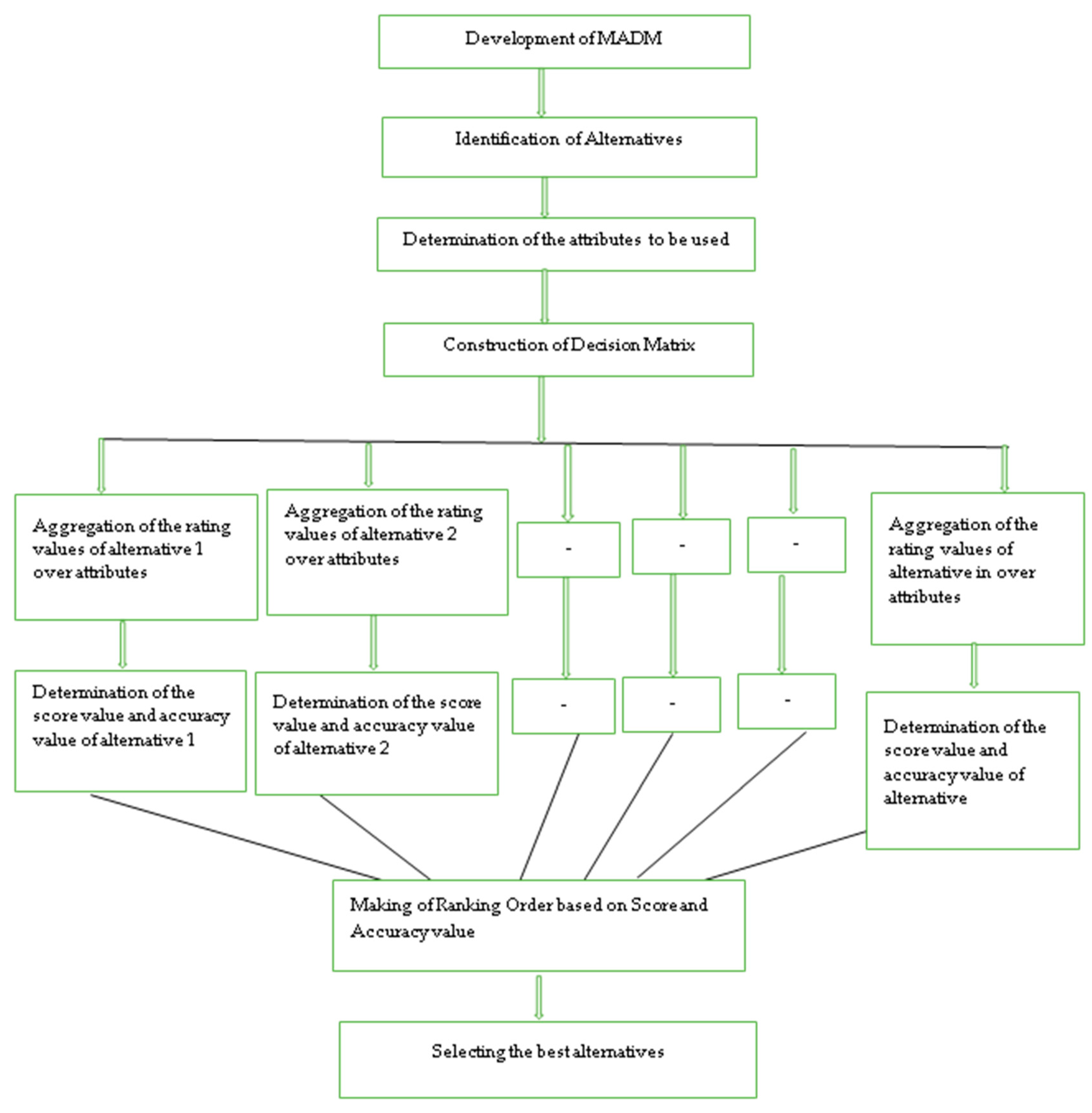
Application of TFNNWA and TFNNWG operators to multi attribute decision makingin which $\stackrel{⃛}{M}=\left\{{\stackrel{⃛}{M}}_1,{\stackrel{⃛}{M}}_2,\dots ,{\stackrel{⃛}{M}}_a\right\}$ is the set ofn possible substitutes and $\stackrel{⃛}{N}=\left\{{\stackrel{⃛}{N}}_1,{\stackrel{⃛}{N}}_2,\dots ,{\stackrel{⃛}{N}}_b\right\}$ is the set of features. Assume that $\stackrel{⃛}{t}={(1/f,1/f,\dots ,1/f)}^{\stackrel{⌣}{T}}$ is the normalized weights of the features, where ${\stackrel{⃛}{t}}_f$ denotes the importance degree of the feature $\stackrel{⃛}{U}={\left({\stackrel{⃛}{h}}_{ef}\right)}_{a\times b}{M}_f(f=1,2,\dots ,b)$ such that ${\stackrel{⃛}{t}}_f\ge 0$ and ${\displaystyle \sum _{f=1}^b{\stackrel{⃛}{t}}_f=1}$ for $(f=1,2,\dots ,b).$ The ratings of all alternatives ${\stackrel{⃛}{M}}_e(e=1,2,\dots ,a)$ with respect to the features ${\stackrel{⃛}{M}}_v(v=1,2,\dots ,y)$ have been presented in aTFNNV based decisionmatrix $\stackrel{⃛}{U}={\left({\stackrel{⃛}{h}}_{uv}\right)}_{x\times y}.$

Based on the TFNNWA and TFNNWG operators, for solving MADM problems we develop a practical approach. In this approach, the ratings of the alternatives over the attributesare expressed with TFNNVs (Figure 1).

Application of the TFNNWA Operator

Step 1. Aggregate the rating values of the substitute $Y_u\left(u=i,ii,iii,iv\right)$ defined in the u-th row of decision matrix $\stackrel{⃛}{k}={({\stackrel{⃛}{k}}_{ef})}_{4\times 5}$ with the TFNNWA operator.

Step 2. The aggregated rating values ${\stackrel{⃛}{h}}_u$ matching to the substitute ${\stackrel{⃛}{Y}}_u$ are computed using Equation (6) which is as defined below:

$$TFNNW{A}_{\stackrel{⃛}{t}}\left({\stackrel{⃛}{M}}_1,{\stackrel{⃛}{M}}_2,\dots ,{\stackrel{⃛}{M}}_f\right)={\stackrel{⃛}{t}}_1{\stackrel{⃛}{M}}_1\widehat{\oplus }{\stackrel{⃛}{t}}_2{\stackrel{⃛}{M}}_2\widehat{\oplus },\dots ,\widehat{\oplus }{\stackrel{⃛}{t}}_f{\stackrel{⃛}{M}}_f=\underset{f=1}{\overset{b}{\widehat{\oplus }}}\left({\stackrel{⃛}{t}}_f{\stackrel{⃛}{M}}_f\right),$$

(6)

Step 3. By Equations (7) and (8) the score and accuracy values of alternatives $Y_u\left(u=i,ii,iii,iv\right)$ are determined, both of which are defined below:

$$\stackrel{⃛}{H}\left({\stackrel{⃛}{K}}_1\right)=\frac{1}{4}\left[\left({\alpha }_1+2{\beta }_1+{\gamma }_1\right)-\left({\chi }_1+2{\lambda }_1+{\delta }_1\right)\right]$$

(7)

$$\stackrel{⃛}{S}\left({\stackrel{⃛}{K}}_1\right)=\frac{1}{12}\left[8+\left({\alpha }_1+2{\beta }_1+{\gamma }_1\right)-\left({\mu }_1+2{\nu }_1+{\rho }_1\right)-\left({\chi }_1+2{\lambda }_1+{\delta }_1\right)\right]$$

(8)

Step 4. In

Table 2. Aggregated rating values of score and accuracy values.

Alternative	Score Values of $\stackrel{⃛}{\mathit{S}}\left({\stackrel{⃛}{\mathit{K}}}_1\right)$	Accuracy Values of $\stackrel{⃛}{\mathit{H}}\left({\stackrel{⃛}{\mathit{K}}}_1\right)$
$Y_i$	0.7960	0.5921
$Y_{ii}$	0.8103	0.6247
$Y_{iii}$	0.6464	0.1864
$Y_{iv}$	0.6951	0.3789

, according to the descending order of the score and accuracy values the order of the substitutes $Y_u\left(u=i,ii,iii,iv\right)$ is determined and is shown.

Therefore, following is the ranking order of the alternatives presented:

$$Y_{ii}\succ Y_i\succ Y_{iv}\succ Y_{iii}.$$

Step 5. The highest ranking order is the best medical representative. In this example, $Y_{ii}$ would be the best candidate for the position of medical representative.

Utilization of TFNNWG Operator

Step 1. By means of Equation (6)

$$TFNN{\mathrm{WG}}_{\stackrel{⌣}{w}}\left({\stackrel{⌣}{A}}_1,{\stackrel{⌣}{A}}_2,\dots ,{\stackrel{⌣}{A}}_m\right)={{\stackrel{⌣}{A}}_1}^{\stackrel{⌣}{\mathrm{w}}1}\otimes {{\stackrel{⌣}{A}}_2}^{\stackrel{⌣}{\mathrm{w}}2}\widehat{\otimes }\dots \widehat{\otimes }{{\stackrel{⌣}{A}}_m}^{\stackrel{⌣}{\mathrm{w}}m}=\underset{q=1}{\overset{m}{\widehat{\otimes }}}\left({{\stackrel{⌣}{A}}_q}^{\stackrel{⌣}{\mathrm{w}}\mathrm{q}}\right),$$

(9)

All the rating values of the alternatives $Y_u\left(u=i,ii,iii,iv\right)$ for the u-th row of the decision matrix $\stackrel{⃛}{k}={({\stackrel{⃛}{k}}_{uv})}_{4\times 5}$ are aggregated.

Step 2. In the

Table 3. Rating values of the aggregated triangular fuzzy number neutrosophic set (TFNN).

Aggregated Rating Values
$u_1\langle \left(0.6654,0.7161,0.7667\right),\left(0.1643,0.2144,0.2626\right),\left(0.1142,0.1643,0.2144\right)\rangle$
$u_2\langle \left(0.6998,0.7502,0.8002\right),\left(0.1485,0.1986,0.2486\right),\left(0.0984,0.1485,0.1986\right)\rangle$
$u_3\langle \left(0.4472,0.4975,0.5477\right),\left(0.3292,0.3795,0.4299\right),\left(0.2789,0.3292,0.3795\right)\rangle$
$u_4\langle \left(0.5291,0.5804,0.6316\right),\left(0.2707,0.3214,0.3721\right),\left(0.2202,0.2707,0.3215\right)\rangle$

, corresponding to the alternative $Y_u$ the aggregated rating values $u_p$ are shown.

Step 3. We will put the Table 2 values in Equations (5) and (6) and the score and accuracy values of substitutes $Y_u(u=i,ii,iii,iv)$ are computed. The results obtained in

Table 4. Score and Accuracy values of rating values.

Alternative	Score Value $\mathit{S}({\mathit{u}}_{\mathit{p}})$	Accuracy Values $\stackrel{⌣}{\mathit{A}}({\mathit{u}}_{\mathit{p}})$
$Y_i$	0.7791	0.5518
$Y_{ii}$	0.8010	0.6016
$Y_{iii}$	0.5962	0.1683
$Y_{iv}$	0.6627	0.3096

are shown below.

Step 4. According to the descending order of the score and accuracy values the order of alternatives $Y_u(u=i,ii,iii,iv)$ has been determined. Following is the ranking order of the alternatives presented:

$$Y_{ii}\succ Y_i\succ Y_{iv}\succ Y_{iii}$$

Step 5. The highest ranking order is the best medical representative. In this example, $Y_{ii}$ would be the best candidate for the position of medical representative.

5. Conclusions

In this paper, we gave an overview of a neutrosophic set, its extensions, and other hybrid frameworks of neutrosophic sets, fuzzy based models soft sets, and the application of these neutrosophic models in (MADM) problems. Further, the theoretical properties of the neutrosophic set with its other counterparts have been discussed. Based on the various instances of neutrosophic sets, decision making algorithms have been reviewed, and the utility of these algorithms have been demonstrated using illustrative examples. Aside from the general neutrosophic set, other instances and extensions of neutrosophic sets that were reviewed in this paper include the SVNS, INS, BNS, GINSS, and RNS.

The decision maker provides the information that is often incomplete, inconsistent, and indeterminate in real situations. For actual, logical, and engineering application, a single-valued neutrosophic set (SVNS) is more accurate, because it can handle all of the above information. SVNS was presented by Wang et al. [14], which is an illustration of NS. The classic set, FS, IVFS, IFS and paraconsistent set are the generalization of the SVNS. The INS was presented by H. Wang [15], which is an instance of NS. The classic set, FS, IVFS, IFS, IVFIS, interval type-2 FS and paraconsistent set are the generalized form of INS. Accuracy, score and certainty functions of a BNS was presented by Deli et al. [12] in which A_w and G_w operators were suggested to aggregate the bipolar neutrosophic information. Then, according to the values of accuracy, score, and certainty, functions of alternatives are ranked to choose the most desirable one(s).

A soft set was first introduced by Molodtsov [54]. In a decision making problem, they defined some operations on GNSS and presented an application of GNSS. The GNSS was extended by Sahin and Küçük [39] to the situation of IVNSS. In dealing with some decision making problems they also gave some application of GINSS. Some basic properties of a neutrosophic refined set were firstly defined by Broumi et al. [61]. A neutrosophic Refined Set (NRS) with a correlation measure was proposed. In a neutrosophic refined set, Surapati et al. [41] developed a MCGDM model and offered its use in teacher selection. In more basic form the tangent similarity function has been presented. To other GDM problems, the suggested method can also be applied under refined neutrosophic set environment.

For dealing with the vagueness and imperfectness of the DMs assessments, the triangular neutrosophic fuzzy number was used. To solve the MADM problem under a neutrosophic environment, aggregation operators were proposed. Finally, with medical representative selection, the efficiency and applicability of the recommended method has been clarified. In other DM problems, the proposed approach can be also applied to personnel selection, medical diagnosis, and pattern recognition [62,63,64,65,66,67,68,69,70,71,72,73,74,75,76,77,78,79,80,81,82,83,84,85,86,87,88,89,90,91,92,93].

References

- Smarandache, F. Neutrosophic set—A generalization of the intuitionistic fuzzy set. Int. J. Pure Appl. Math. 2004, 24, 287. [Google Scholar]
- Atanassov, K.T. Intuitionistic fuzzy sets. Fuzzy Sets Syst. 1986, 20, 87–96. [Google Scholar] [CrossRef]
- Smarandache, F. Neutrosophy: A Unifying Field in Logics: Neutrosophic Logic. Neutrosophy, Neutrosophic Set, Neutrosophic Probability; American Research Press: Rehoboth, NM, USA, 2005. [Google Scholar]
- Wang, H.; Smarandache, F.; Zhang, Y.; Sunderraman, R. Single valued neutrosophic sets. In Proceedings of the 10th International. Conference on Fuzzy Theory and Technology, Salt Lake City, UT, USA, 21–26 July 2005. [Google Scholar]
- Wang, H.; Madiraju, P.; Zhang, Y.; Sunderraman, R. Interval neutrosophic sets. arXiv, 2004; arXiv:math/0409113. [Google Scholar]
- Maji, P.K. Neutrosophic soft set. Ann. Fuzzy Math. Inform. 2013, 5, 157–168. [Google Scholar]
- Broumi, S.; Smarandache, F. Intuitionistic neutrosophic soft set. J. Comput. Inf. Sci. Eng. 2013, 8, 130–140. [Google Scholar]
- Broumi, S.; Smarandache, F.; Dhar, M. Rough neutrosophic sets. Neutrosophic Sets Syst. 2014, 3, 62–67. [Google Scholar]
- Broumi, S.; Smarandache, F. Interval valued neutrosophic rough set. J. New Res. Sci. 2014, 7, 58–71. [Google Scholar]
- Broumi, S.; Smarandache, F. Interval valued neutrosophic soft rough set. Int. J. Comput. Math. 2015, 2015. [Google Scholar] [CrossRef]
- Ali, M.; Smarandache, F. Complex neutrosophic set. Neural Comput. Appl. 2017, 28, 1817–1834. [Google Scholar] [CrossRef]
- Deli, I.; Ali, M.; Smarandache, F. Bipolar neutrosophic sets and their application based on multi-criteria decision making problems. In Proceedings of the 2015 International Conference on Advanced Mechatronic Systems (ICAMechS), Beijing, China, 22–24 August 2015; pp. 249–254. [Google Scholar]
- Ali, M.; Deli, I.; Smarandache, F. The theory of neutrosophic cubic sets and their applications in pattern recognition. J. Intell. Fuzzy Syst. 2016, 30, 1957–1963. [Google Scholar] [CrossRef]
- Wang, H.; Smarandache, F.; Zhang, Y.; Sunderraman, R. Single valued neutrosophic sets. Rev. Air Force Acad. 2010, 1, 10. [Google Scholar]
- Wang, H.; Smarandache, F.; Sunderraman, R.; Zhang, Y.Q. Interval Neutrosophic Sets and Logic: Theory and Applications in Computing; Hexis: Phoenix, AR, USA, 2005; Volume 5. [Google Scholar]
- Biswas, P.; Pramanik, S.; Giri, B.C. TOPSIS method for multi-attribute group decision making under single-valued neutrosophic environment. Neural Comput. Appl. 2016, 27, 727–737. [Google Scholar] [CrossRef]
- Ye, J. Multi-criteria decision making method using the correlation coefficient under single-valued neutrosophic environment. Int. J. Gen. Syst. 2013, 42, 386–394. [Google Scholar] [CrossRef]
- Deli, I.; Subas, Y. Single valued neutrosophic numbers and their applications to multicriteria decision making problem. Neutrosophic Sets Syst. 2014, 2, 1–13. [Google Scholar]
- Huang, H. New distance measure of single-valued neutrosophic sets and its application. Int. J. Intell. Syst. 2016, 31, 1021–1032. [Google Scholar] [CrossRef]
- Yang, L.; Li, B. A Multi-Criteria Decision-Making Method Using Power Aggregation Operators for Single-valued Neutrosophic Sets. Int. J. Database Theory Appl. 2016, 9, 23–32. [Google Scholar] [CrossRef]
- Ye, J. Single valued neutrosophic cross-entropy for multi-criteria decision making problems. Appl. Math. Model. 2014, 38, 1170–1175. [Google Scholar] [CrossRef]
- Deli, I.; Şubaş, Y. A ranking method of single valued neutrosophic numbers and its applications to multi-attribute decision making problems. Int. J. Mach. Learn. Cybern. 2017, 8, 1309–1322. [Google Scholar] [CrossRef]
- Ye, J. Improved correlation coefficients of single valued neutrosophic sets and interval neutrosophic sets for multiple attribute decision making. J. Intell. Fuzzy Syst. 2014, 27, 2453–2462. [Google Scholar]
- Ye, J.; Zhang, Q. Single valued neutrosophic similarity measures for multiple attribute decision making. Neutrosophic Sets Syst. 2014, 2, 48–54. [Google Scholar]
- Ye, J. An extended TOPSIS method for multiple attribute group decision making based on single valued neutrosophic linguistic numbers. J. Intell. Fuzzy Syst. 2015, 28, 247–255. [Google Scholar]
- Ye, J. Improved cross entropy measures of single valued neutrosophic sets and interval neutrosophic sets and their multicriteria decision making methods. Cybern. Inf. Technol. 2015, 15, 13–26. [Google Scholar] [CrossRef]
- Ye, J.; Fu, J. Multi-period medical diagnosis method using a single valued neutrosophic similarity measure based on tangent function. Comput. Methods Programs Biomed. 2016, 123, 142–149. [Google Scholar] [CrossRef] [PubMed]
- Sahin, R.; Karabacak, M. A multi attribute decision making method based on inclusion measure for interval neutrosophic sets. Int. J. Eng. Appl. Sci. 2015, 2, 13–15. [Google Scholar]
- Chi, P.; Liu, P. An extended TOPSIS method for the multiple attribute decision making problems based on interval neutrosophic set. Neutrosophic Sets Syst. 2013, 1, 63–70. [Google Scholar]
- Huang, Y.; Wei, G.; Wei, C. VIKOR method for interval neutrosophic multiple attribute group decision-making. Information 2017, 8, 144. [Google Scholar] [CrossRef]
- Liu, P.; Wang, Y. Interval neutrosophic prioritized OWA operator and its application to multiple attribute decision making. J. Syst. Sci. Complex. 2016, 29, 681–697. [Google Scholar] [CrossRef]
- Tian, Z.P.; Zhang, H.Y.; Wang, J.; Wang, J.Q.; Chen, X.H. Multi-criteria decision-making method based on a cross-entropy with interval neutrosophic sets. Int. J. Syst. Sci. 2016, 47, 3598–3608. [Google Scholar] [CrossRef]
- Ye, J. Similarity measures between interval neutrosophic sets and their applications in multi-criteria decision making. J. Intell. Fuzzy Syst. 2014, 26, 165–172. [Google Scholar]
- Zhang, H.Y.; Wang, J.Q.; Chen, X.H. Interval neutrosophic sets and their application in multi-criteria decision making problems. Sci. World J. 2014, 2014, 1–15. [Google Scholar]
- Zhang, H.Y.; Ji, P.; Wang, J.Q.; Chen, X.H. An improved weighted correlation coefficient based on integrated weight for interval neutrosophic sets and its application in multi-criteria decision-making problems. Int. J. Comput. Intell. Syst. 2015, 8, 1027–1043. [Google Scholar] [CrossRef]
- Dey, P.P.; Pramanik, S.; Giri, B.C. TOPSIS for Solving Multi-Attribute Decision Making Problems under Bi-Polar Neutrosophic Environment. In New Trends in Neutrosophic Theory and Applications; Smarandache, F., Pramanik, S., Eds.; Pons asbl: Brussels, Belgium, 2016; p. 65. [Google Scholar]
- Ali, M.; Son, L.H.; Deli, I.; Tien, N.D. Bipolar neutrosophic soft sets and applications in decision making. J. Intell. Fuzzy Syst. 2017, 33, 4077–4087. [Google Scholar] [CrossRef]
- Uluçay, V.; Deli, I.; Şahin, M. Similarity measures of bipolar neutrosophic sets and their application to multiple criteria decision making. Neural Comput. Appl. 2018, 29, 739–748. [Google Scholar] [CrossRef]
- Sahin, R.; Küçük, A. Generalised Neutrosophic Soft Set and its Integration to Decision Making Problem. Appl. Math. Inf. Sci. 2014, 8, 2751–2759. [Google Scholar] [CrossRef]
- Broumi, S.; Sahin, R.; Smarandache, F. Generalized interval neutrosophic soft set and its decision making problem. J. New Res. Sci. 2014, 3, 29–47. [Google Scholar]
- Mondal, K.; Pramanik, S. Neutrosophic refined similarity measure based on cotangent function and its application to multi-attribute decision making. J. New Theory 2015, 8, 41–50. [Google Scholar]
- Samuel, A.E.; Narmadhagnanam, R. Neutrosophic refined sets in medical diagnosis. Int. J. Fuzzy Math. Arch. 2017, 14, 117–123. [Google Scholar]
- Pramanik, S.; Banerjee, D.; Giri, B. TOPSIS Approach for Multi Attribute Group Decision Making in Refined Neutrosophic Environment. In New Trends in Neutrosophic Theory and Applications; Smarandache, F., Pramanik, S., Eds.; Pons asbl: Brussels, Belgium, 2016. [Google Scholar]
- Chen, J.; Ye, J.; Du, S. Vector similarity measures between refined simplified neutrosophic sets and their multiple attribute decision-making method. Symmetry 2017, 9, 153. [Google Scholar] [CrossRef]
- Biswas, P.; Pramanik, S.; Giri, B.C. Aggregation of triangular fuzzy neutrosophic set information and its application to multi-attribute decision making. Neutrosophic Sets Syst. 2016, 12, 20–40. [Google Scholar]
- Zhang, X.; Liu, P. Method for aggregating triangular fuzzy intuitionistic fuzzy information and its application to decision making. Technol. Econ. Dev. Econ. 2010, 16, 280–290. [Google Scholar] [CrossRef] [Green Version]
- Biswas, P.; Pramanik, S.; Giri, B.C. Cosine similarity measure based multi-attribute decision-making with trapezoidal fuzzy neutrosophic numbers. Neutrosophic Sets Syst. 2014, 8, 46–56. [Google Scholar]
- Ye, J. Trapezoidal neutrosophic set and its application to multiple attribute decision making. Neural Comput. Appl. 2015, 26, 1157–1166. [Google Scholar] [CrossRef]
- Mondal, K.; Surapati, P.; Giri, B.C. Role of Neutrosophic Logic in Data Mining. In New Trends in Neutrosophic Theory and Applications; Smarandache, F., Pramanik, S., Eds.; Pons asbl: Brussels, Belgium, 2016; pp. 15–23. [Google Scholar]
- Radwan, N.M. Neutrosophic Applications in E-learning: Outcomes, Challenges and Trends. In New Trends in Neutrosophic Theory and Applications; Smarandache, F., Pramanik, S., Eds.; Pons asbl: Brussels, Belgium, 2016; pp. 177–184. [Google Scholar]
- Koundal, D.; Gupta, S.; Singh, S. Applications of Neutrosophic Sets in Medical Image Diagnosing and segmentation. In New Trends in Neutrosophic Theory and Applications; Smarandache, F., Pramanik, S., Eds.; Pons asbl: Brussels, Belgium, 2016; pp. 257–275. [Google Scholar]
- Patro, S.K. On a Model of Love dynamics: A Neutrosophic analysis. In New Trends in Neutrosophic Theory and Applications; Smarandache, F., Pramanik, S., Eds.; Pons asbl: Brussels, Belgium, 2016; pp. 279–287. [Google Scholar]
- Zadeh, L.A. Fuzzy Sets. Inf. Control 1965, 8, 338–353. [Google Scholar] [CrossRef]
- Molodtsov, D. Soft set theory—First result. Comput. Math. Appl. 1999, 37, 19–31. [Google Scholar] [CrossRef]
- Karaaslan, F. Correlation coefficients of single-valued neutrosophic refined soft sets and their applications in clustering analysis. Neural Comput. Appl. 2017, 28, 2781–2793. [Google Scholar]
- Broumi, S.; Smarandache, F. Extended Hausdorff distance and similarity measures for neutrosophic refined sets and their application in medical diagnosis. J. New Theory 2015, 7, 64–78. [Google Scholar]
- Boran, F.E.; Genç, S.; Kurt, M.; Akay, D. A multi-criteria intuitionistic fuzzy group decision making for supplier selection with TOPSIS method. Expert Syst. Appl. 2009, 36, 11363–11368. [Google Scholar] [CrossRef]
- Dezert, J. Open Questions on Neutrosophic Inference. Mult.-Valued Log. 2002, 8, 439–472. [Google Scholar]
- Wang, Y.M. Using the method of maximizing deviations to make decision for multi-indices. Syst. Eng. Electron. 1998, 7, 31. [Google Scholar]
- Nădăban, S.; Dzitac, S. Neutrosophic TOPSIS: A general view. In Proceedings of the 2016 6th International Conference on Computers Communications and Control (ICCCC), Oradea, Romania, 10–14 May 2016; pp. 250–253. [Google Scholar]
- Broumi, S.; Smarandache, F. Neutrosophic refined similarity measure based on cosine function. Neutrosophic Sets Syst. 2014, 6, 42–48. [Google Scholar]
- Broumi, S.; Smarandache, F. Correlation coefficient of interval neutrosophic set. In Applied Mechanics and Materials; Trans Tech Publications, Inc.: Zürich, Switzerland, 2013; pp. 511–517. [Google Scholar]
- Broumi, S.; Smarandache, F. More on intuitionistic neutrosophic soft sets. Comput. Sci. Inf. Technol. 2013, 1, 257–268. [Google Scholar]
- Ali, M.; Son, L.H.; Thanh, N.D.; Nguyen, V.M. A neutrosophic recommender system for medical diagnosis based on algebraic neutrosophic measures. Appl. Soft Comput. 2018. [Google Scholar] [CrossRef]
- Al-Quran, A.; Hassan, N. Fuzzy parameterized single valued neutrosophic soft expert set theory and its application in decision making. Int. J. Appl. Decis. Sci. 2016, 9, 212–227. [Google Scholar]
- Ansari, A.Q.; Biswas, R.; Aggarwal, S. Proposal for applicability of neutrosophic set theory in medical AI. Int. J. Comput. Appl. 2011, 27, 5–11. [Google Scholar] [CrossRef]
- Bhowmik, M.; Pal, M. Intuitionistic neutrosophic set relations and some of its properties. J. Comput. Inform. Sci. 2010, 5, 183–192. [Google Scholar]
- Biswas, R.; Pandey, U.S. Neutrosophic Relational Database Decomposition. Int. J. Adv. Comput. Sci. Appl. 2011, 2, 121–125. [Google Scholar]
- Broumi, S.; Smarandache, F. Cosine similarity measure of interval valued neutrosophic sets. Neutrosophic Sets Syst. 2014, 5, 15–20. [Google Scholar]
- Broumi, S.; Smarandache, F. Several similarity measures of neutrosophic sets. Neutrosophic Sets Syst. 2013, 1, 54–62. [Google Scholar]
- Broumi, S.; Deli, I.; Smarandache, F. Neutrosophic parameterized soft set theory and its decision making. Ital. J. Pure Appl. Math. 2014, 32, 503–514. [Google Scholar]
- Deli, I.; Broumi, S.; Smarandache, F. On neutrosophic refined sets and their applications in medical diagnosis. J. New Theory 2015, 6, 88–98. [Google Scholar]
- Karaaslan, F. Possibility neutrosophic soft sets and PNS-decision making method. Appl. Soft Comput. 2017, 54, 403–414. [Google Scholar] [CrossRef]
- Maji, P.K. A neutrosophic soft set approach to a decision making problem. Ann. Fuzzy Math Inform. 2012, 3, 313–319. [Google Scholar]
- Pawlak, Z.; Grzymala-Busse, J.; Slowinski, R.; Ziarko, W. Rough sets. Commun. ACM 1995, 38, 88–95. [Google Scholar] [CrossRef]
- Peng, X.; Liu, C. Algorithms for neutrosophic soft decision making based on EDAS, new similarity measure and level soft set. J. Intell. Fuzzy Syst. 2017, 32, 955–968. [Google Scholar] [CrossRef]
- Peng, J.J.; Wang, J.; Wang, J.; Zhang, H.; Chen, X. Simplified neutrosophic sets and their applications in multi-criteria group decision-making problem. Int. J. Syst. Sci. 2016, 47, 2342–2358. [Google Scholar] [CrossRef]
- Sahin, R.; Liu, P. Maximizing deviation method for neutrosophic multiple attribute decision making with incomplete weight information. Neural Comput. Appl. 2015, 27, 2017–2029. [Google Scholar] [CrossRef]
- Schweizer, B.; Sklar, A. Statistical metric spaces. Pac. J. Math. 1960, 10, 313–334. [Google Scholar] [CrossRef] [Green Version]
- Thanh, N.D.; Ali, M.; Son, L.H. A novel clustering algorithm in a neutrosophic recommender system for medical diagnosis. Cogn. Comput. 2017, 9, 526–544. [Google Scholar] [CrossRef]
- Ye, J. A multi-criteria decision making method using aggregation operators for simplified neutrosophic sets. J. Intell. Fuzzy Syst. 2014, 26, 2459–2466. [Google Scholar]
- Ye, J. Fault diagnoses of hydraulic turbine using the dimension root similarity measure of single-valued neutrosophic sets. Intell. Autom. Soft Comput. 2016, 1–8. [Google Scholar] [CrossRef]
- Ye, J. Single-valued neutrosophic similarity measures based on cotangent function and their application in the fault diagnosis of steam turbine. Soft Comput. 2017, 21, 817–825. [Google Scholar] [CrossRef]
- Ye, J.; Du, S. Some distances, similarity and entropy measures for interval valued neutrosophic sets and their relationship. Int. J. Mach. Learn. Cybern. 2017, 1–9. [Google Scholar] [CrossRef]
- Zhang, C.; Zhai, Y.; Li, D.; Mu, Y. Steam turbine fault diagnosis based on single-valued neutrosophic multigranulation rough sets over two universes. J. Intell. Fuzzy Syst. 2016, 31, 2829–2837. [Google Scholar] [CrossRef]
- Zhang, C.; Li, D.; Sangaiah, A.K.; Broumi, S. Merger and acquisition target selection based on interval neutrosophic multi-granulation rough sets over two universes. Symmetry 2017, 9, 126. [Google Scholar] [CrossRef]
- Jha, S.; Kumar, R.; Son, L.; Chatterjee, J.M.; Khari, M.; Yadav, N.; Smarandache, F. Neutrosophic soft set decision making for stock trending analysis. Evolv. Syst. 2018. [Google Scholar] [CrossRef]
- Dey, A.; Broumi, S.; Son, L.H.; Bakali, A.; Talea, M.; Smarandache, F. A new algorithm for finding minimum spanning trees with undirected neutrosophic graphs. Granul Comput. 2018, 1–7. [Google Scholar] [CrossRef]
- Ali, M.; Son, L.H.; Khan, M.; Tung, N.T. Segmentation of dental X-ray images in medical imaging using neutrosophic orthogonal matrices. Expert Syst. Appl. 2018, 91, 434–441. [Google Scholar] [CrossRef]
- Ali, M.; Dat, L.Q.; Son, L.H.; Smarandache, F. Interval complex neutrosophic set: Formulation and applications in decision-making. Int. J. Fuzzy Syst. 2018, 20, 986–999. [Google Scholar] [CrossRef]
- Nguyen, G.N.; Son, L.H.; Ashour, A.S.; Dey, N. A survey of the state-of-the-arts on neutrosophic sets in biomedical diagnoses. Int. J. Mach. Learn. Cybern. 2017, 1–13. [Google Scholar] [CrossRef]
- Thanh, N.D.; Son, L.H.; Ali, M. Neutrosophic recommender system for medical diagnosis based on algebraic similarity measure and clustering. In Proceedings of the 2017 IEEE International Conference on Fuzzy Systerm (FUZZ-IEEE), Naples, Italy, 9–12 July 2017; pp. 1–6. [Google Scholar]
- Broumi, S.; Bakali, A.; Talea, M.; Smarandache, F.; Selvachandran, G. Computing Operational Matrices in Neutrosophic Environments: A Matlab Toolbox. Neutrosophic Sets Syst. 2017, 18, 58–66. [Google Scholar]
Figure 1.
Framework for the proposed multiple attribute decision-making (MADM) method.