Article

The Effect of Land Use on Availability of Japanese Freshwater Resources and Its Significance for Water Footprinting

1
Research Institute of Science for Safety and Sustainability, National Institute of Advanced Industrial Science and Technology, 16-1, Onogawa, Tsukuba, Ibaraki 305-8569, Japan
2
Institute of Industrial Science, The University of Tokyo, 4-6-1, Komaba, Meguro-ku, Tokyo 153-8505, Japan
3
Chair of Sustainable Engineering, Technische Universität Berlin, Strasse des 17. Juni 135, Berlin 10623, Germany
4
School of Advanced Engineering, Kogakuin University, 1-24-2, Nishi-shinjuku, Shinjuku-ku, Tokyo 163-8677, Japan
*
Author to whom correspondence should be addressed.
Sustainability 2016, 8(1), 86; https://doi.org/10.3390/su8010086
Submission received: 19 October 2015 / Revised: 14 December 2015 / Accepted: 12 January 2016 / Published: 16 January 2016

Abstract

:
All relevant effects on water must be assessed in water footprinting for identifying hotspots and managing the impacts of products, processes, and services throughout the life cycle. Although several studies have focused on physical water scarcity and degradation of water quality, the relevance of land use in water footprinting has not been widely addressed. Here, we aimed to verify the extent of land-use effect in the context of water footprinting. Intensity factors of land use regarding the loss of freshwater availability are modeled by calculating water balance at grid scale in Japan. A water footprint inventory and impacts related to land use are assessed by applying the developed intensity factors and comparing them with those related to water consumption and degradation. Artificial land use such as urban area results in the loss of many parts of available freshwater input by precipitation. When considering water footprint inventory, the dominance of land use is less than that of water consumption. However, the effect of land use is relevant to the assessment of water footprint impact by differentiating stress on water resources. The exclusion of land use effect underestimates the water footprint of goods produced in Japan by an average of around 37%.

1. Introduction

Freshwater is a necessary resource for sustaining healthy human life and ecosystems. Although water covers major parts of the globe, available freshwater resources are only limited to ~0.8% of total water resources [1]. Population growth increases water demand and leads to competition for freshwater use. Imbalance of demand and supply of freshwater has various environmental impacts owing to freshwater use. In addition, both availability and demand of freshwater resources vary by region, which means that the stress of freshwater scarcity is not geographically uniform. Recent globalized supply chains of products and services increases the complexity and difficulties of identifying and managing critical environmental impacts of water use in those chains. In this context, a special type of Life Cycle Assessment (LCA) that focuses on the potential environmental impacts relevant to water use has attracted attention as water footprinting. Water footprinting is a technique to assess and understand water related impacts of products, processes, and organizations through their life cycle on the basis of LCA. Therefore, water footprinting can be a tool for tracing the environmental impacts of water use through life cycle of products, processes and organizations and expected to contribute to improved water management in terms of environmental impacts.
According to the ISO standard, water footprinting targets all kinds of relevant causes affecting water availability [2]. Physical scarcity caused by water withdrawal and consumption is not the only issue relevant to water availability. Water degradation caused by physical and chemical changes of components also directly influences that availability. Land use indirectly impacts the availability of water resources (surface and ground water) by altering the water cycle. In principle, these relevant issues should be considered in water footprinting [2].
Methods for addressing the impacts of water use have been developed in the context of water footprinting [3]. Regarding impacts related to physical scarcity by direct water use, there are many methods already developed. A consensual method is now being developed by consensus of various experts and stakeholders toward aggregating current knowledge and providing a single assessment model that can be used widely in practice [4]. For water degradation, several methods have been advanced as tools for assessing the impacts of water pollution, mainly by chemical substances [5]. Recently, the target emissions in the assessment of water degradation have been expanded to thermal emissions and suspended solids [6,7,8]. One method expresses the effects of pollution on water degradation by a proxy that is the assumed volume of water needed to dilute emissions to the concentration in the natural environment [9]. There are also many methods that address the impacts of land use in the context of life cycle assessment and footprinting [10]. However, the relationship between land use and freshwater availability have been modeled and discussed in only limited frontier studies [11,12,13,14]. Ridoutt et al. (2010) and Núñez et al. (2013) focused on green water flow change caused by land use for crop production and evaluated the significance of land use effects on green water availability in comparison with natural reference vegetation [11,12]. Quinteiro et al. (2015) proposed the methods to assess the impacts of land use on not only green water flow but also surface runoff flow and revealed the relative significance of surface runoff flow change associated with land use than green water flow through a case study [13]. Milà i Canals et al. (2010) also suggested the importance of infiltration to groundwater and surface runoff change arose from artificial land use in the context of freshwater use impacts in LCA [14]. While generic data on the effects of land use on the loss of precipitation was indicated [14], specific characterization factors for assessing the impacts of land use on the availability of groundwater and surface water were not developed due to site specific conditions of water flow.
The aim of our study was to verify the significance of land-use effects on freshwater availability in the context of water footprinting. Site-specific water balance calculation which corresponded to artificial land use was necessary to achieve this goal. Thus, the effects of freshwater resource availability in Japan related to land-cover change caused by artificial land use were analyzed by calculating water balance at grid scale for the whole Japanese land area. Based on the results, the significance of land use in the context of water footprinting was verified by calculating the water footprint of goods produced in Japan and comparing with two types of water footprint (consumption and pollution of freshwater).

2. Methods of Analysis

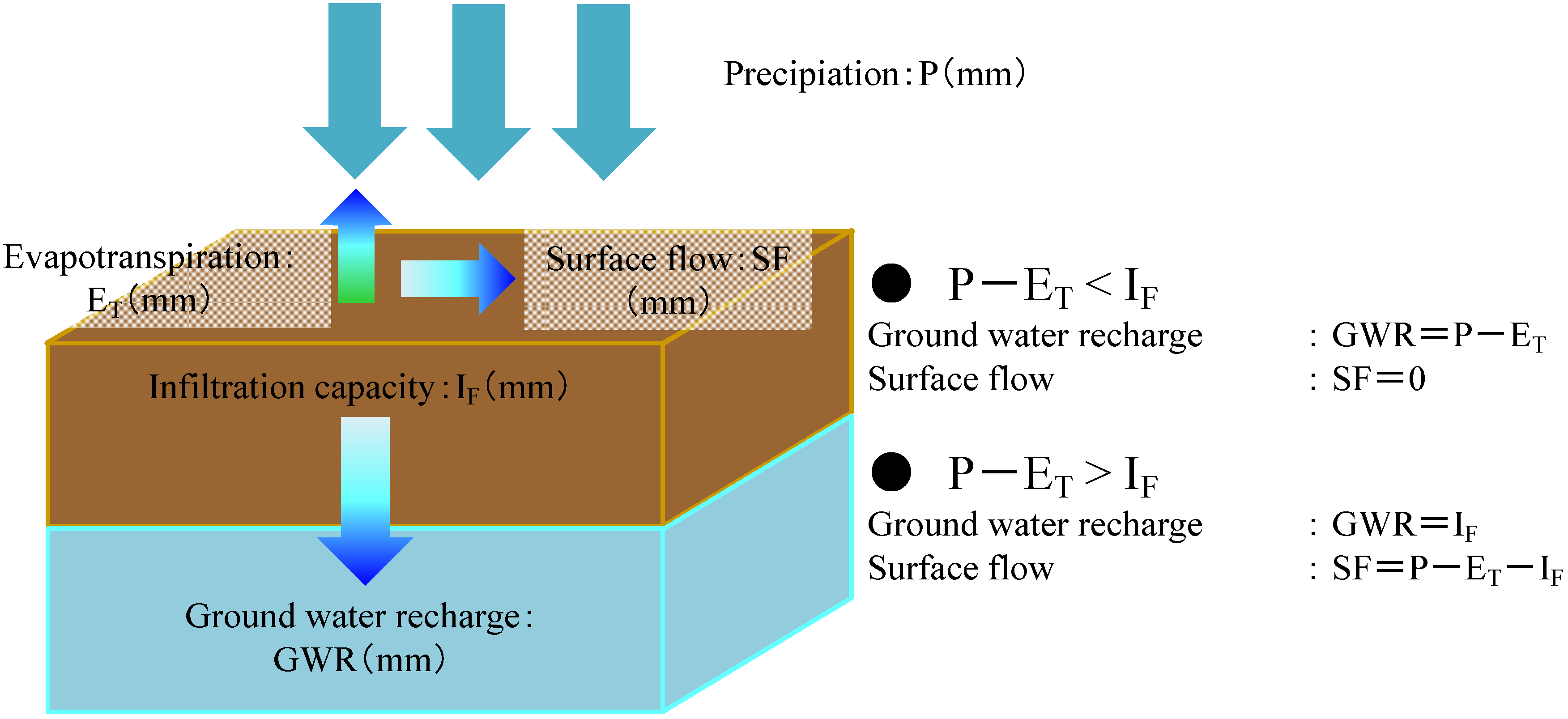
2.1. Water Balance Model for Assessing Availability of Freshwater Resources

The primary source of freshwater for human society and ecosystems is precipitation. Some portion of precipitation evaporates into the atmosphere and the rest infiltrates the ground or floods the ground as surface flow. Artificial land use changes the condition of the ground surface cover and varies the amount of infiltration to groundwater and surface flow. The availability of groundwater and surface water is affected by artificial land use. Changes of groundwater recharge and surface water flow by volume were analyzed by calculating water balance at grid scale (Figure 1).
Figure 1. Schematic diagram of water balance model and calculation on grid.
Sustainability 08 00086 g001
The analysis was done for all land area in Japan on a cell with resolution 1 km × 1 km. The amount of precipitation was from meteorological data [15]. Potential evapotranspiration was estimated via the Thornthwaite equation [16], using meteorological data of average daily temperature and average length of day [15]. The difference between precipitation and evapotranspiration infiltrates the ground and recharges groundwater. However, if that difference exceeds the maximum infiltration capacity of the ground, a surplus water volume floods the ground as surface flow. That capacity is determined in the next Section 2.2 and depends on land use type. Volumes of groundwater recharge and surface flow were calculated on each cell (1 km × 1 km) for whole Japan (377,972 km2) based on daily meteorological data (precipitation, temperature, and length of day) and aggregated as annual water amounts (m3/year).

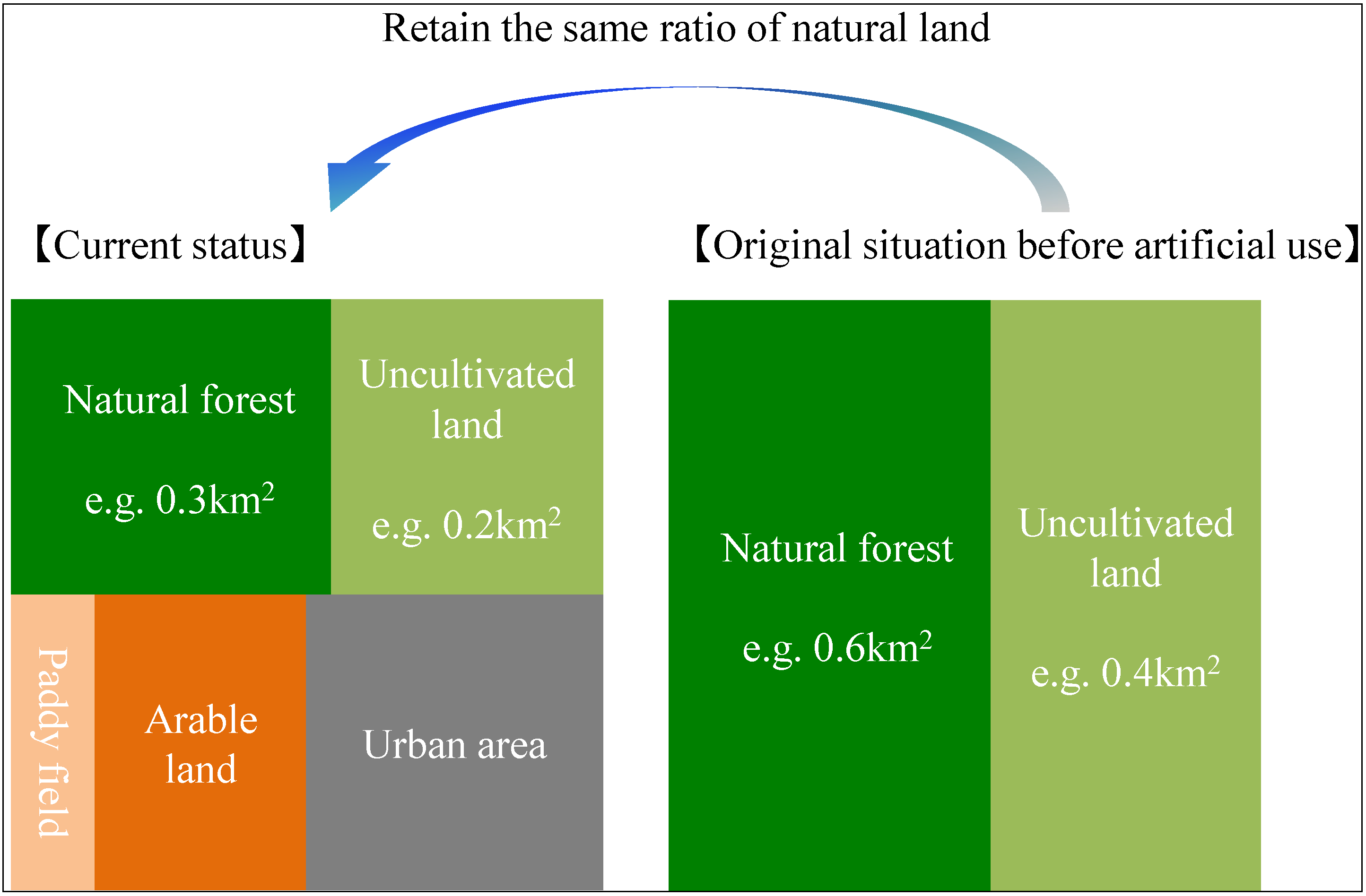
2.2. Classification of Land-Use Type

Six land-use types were defined (natural forest, uncultivated field, planted forest, paddy field, arable land, urban area), corresponding to the land-use classification in Japanese digital map information; areas of each land use at a cell refer to the database with that information [15]. Although there is no robust information on the original state of “natural land”, natural forest and uncultivated fields can be defined as such land, which is unaffected by any artificial land use. Therefore, it was assumed that the proportion of natural forest and uncultivated fields was unchanged from the original situation (Figure 2). The rest of the land-use types (planted forest, paddy field, arable land, urban area) according to the classification of Japanese digital map information were defined as “artificial land” in this study. Based on this premise, changes of groundwater recharge and surface flow were calculated by comparison with the original situation. In the database of digital map information, natural forest and planted forest are not distinguished. Prefectural data of average proportion of planted forest area was used to differentiate the areas of natural and planted forest [17]. The infiltration capacity and maximum evapotranspiration ratio for each land-use type were determined according to representative data based on measurement [18], as shown in Table 1.
Figure 2. Conceptual example of the assumption for the original state of natural land on each cell.
Sustainability 08 00086 g002
Table 1. Infiltration capacity and maximum evapotranspiration ratio for each land-use type.
Land Use TypeInfiltration Capacity (mm/h)Maximum Evapotranspiration Ratio (Dimensionless)
Natural forest2661.2
Uncultivated land1021
Planted forest2661.2
Paddy field89.3 * (except June through August) 1
0.167 (June through August)
Arable land89.31
Urban area15.3 **0.9
* The same infiltration capacity as arable land was used, except for irrigation period; ** Uncovered area by artificial objects (means grass land and bare land) was assumed to be 15% of urban area. For uncovered area, the same infiltration capacity as uncultivated land was used.

2.3. Availability Assessment of Groundwater Recharge and Surface Flow

The amount of groundwater recharge is stored in the ground and remains for a long period, because of a residence time around 100–10,000 years [19]. Surface flow on the ground discharges into rivers and lakes/reservoirs. The average residence time in rivers is shorter (~2–6 months) than in lakes (~50–100 years) [19]. Considering the above, the availability of groundwater recharge and surface flow is obviously different. Even though the range of residence time in groundwater and lakes is wide because of site specific conditions, the results of previous studies support that residence time in groundwater and lakes is generally longer than one year in Japan [20,21,22]. Given the temporal resolution of the present study (one year), freshwater in groundwater and surface flow discharge into lakes has sufficiently long residence times for availability within one year. However, the average residence time of surface flow discharge into rivers is ~4 months (2–6 months), which suggests an availability of 1/3 for one year. The proportion of withdrawal from rivers to total withdrawal from surface water has been calculated around 0.79, according to Japanese statistics [23,24,25]. The amount of available water in surface flow and groundwater recharge is calculated by the following equations.
ASWi,j = SFi,j × 0.79 × 1/3 + SFi,j × (1 − 0.79)
AGWi,j = GWRi,j
where i is the cell identifier; j is the land-use type identifier; ASWi,j is the amount of available water in surface flow for land-use type j on cell i (m3/m2); SFi,j is the amount of surface flow for land-use type j on cell i (m3/m2); AGWi,j is the amount of available water in groundwater recharge for land-use type j on cell i (m3/m2); GWRi,j is the amount of groundwater recharge for land-use type j on cell i (m3/m2).

2.4. Intensity Factors of Availability Loss of Freshwater Caused by Land Use

Intensity factors of availability loss of freshwater caused by land use were calculated for each type of land use. Differences of available water amount between the original situation and each land use type were determined as those intensity factors. As mentioned in Section 2.2, all area in each cell is occupied by natural forest and uncultivated land in the original situation, and the ratio of areas of both land-use types was unchanged for the current situation. Thus, the amount of available water in the original situation can be estimated by the following equations.
ASWi,org = ASWi,NF × Ai,NF / (Ai,NF + Ai,UL) + ASWi,UL × Ai,UL / (Ai,NF + Ai,UL)
AGWi,org = AGWi,NF × Ai,NF / (Ai,NF + Ai,UL) + AGWi,UL × Ai,UL / (Ai,NF + Ai,UL)
where ASWi,org is the amount of available water in surface flow in the original situation on cell i (m3/m2); ASWi,NF is the amount of available water in surface flow for natural forest on cell i (m3/m2); ASWi,UL is the amount of available water in surface flow for uncultivated land on cell i (m3/m2); Ai,NF is the area of natural forest on cell i (m2); Ai,UL is the area of uncultivated land on cell i (m2); AGWi,org is the amount of available water in groundwater recharge in the original situation on cell i (m3/m2); AGWi,NF is the amount of available water in groundwater recharge for natural forest on cell i (m3/m2); AGWi,UL is the amount of available water in groundwater recharge for uncultivated land on cell i (m3/m2).
The lost quantity of freshwater and the intensity factors of availability loss of freshwater corresponding to each type of land use are calculated by the following.
IFLUSWi,j = ASWi,jASWi,org
IFLUGWi,j = AGWi,jAGWi,org
where IFLUSWi,j is the amount of lost surface water with land-use type j on cell i (m3/m2); IFLUGWi,j is the amount of lost groundwater with land-use type j on cell i (m3/m2).

2.5. Calculation of Water Footprint of Goods Produced in Japan

The significance of land use in the context of water footprinting was verified by calculating and comparing water footprints of goods produced in Japan, for three different causes. Those were water consumption from withdrawal, water degradation by pollution, and land use. Information on the volume of water consumption, amount of emissions to water, and land area occupied for production through the supply chain of goods is necessary for comparison of water footprints. Input-output analysis based databases of water consumption [26], water pollution [27], and land use [28] are used as inventories for calculating water footprints related to water consumption, degradation, and land use. These databases apply input-output analysis in the calculation of inventories of all goods produced in Japan. The volume of water consumed related to goods production is accounted for as the water footprint inventory from water consumption [26]. For water degradation, the volume of water for diluting emissions to the level of concentration required by Japanese environmental regulation is used as a proxy of water availability loss caused by pollution [25]. Thus, the water footprint of water degradation is expressed in volumetric figures. The inventory of land area for various types of land use [28] is converted to the volume of lost available water by applying the intensity factors for each type of land use. Those factors are calculated on each cell by Equations (5) and (6), but the inventory of land area use is average data for the entire area of Japan. Therefore, the average intensity factor of all cells is used for the conversion of land area to volume of lost available water attributed to land use.
Although both surface and groundwater are freshwater resources, their scarcity is not identical because of different demands and available water. For impact assessment, these differences of scarcity are considered by applying the ratio of demand to available water as a simple index for assessing the stress of water scarcity. The amounts of withdrawal from surface and groundwater were determined as 73 and 16 billion m3, whereas the amounts of available water in surface and ground water were estimated at 420 and 27 billion m3, respectively [29]. Thus, water scarcity indices of 0.17 for surface water and 0.70 for groundwater were used for assessing the water footprint by multiplying with water volumes in each water footprint inventory. The inventory of water consumption was already differentiated between surface and ground water [26]. The availability loss of freshwater from land use was also different between surface and ground water. However, volumes of dilution water in water degradation do not specify the water sources. Therefore, the ratios of withdrawals from surface and ground water to the total withdrawal were used to differentiate the sources of dilution water in water degradation between surface and ground water.

3. Results and Discussion

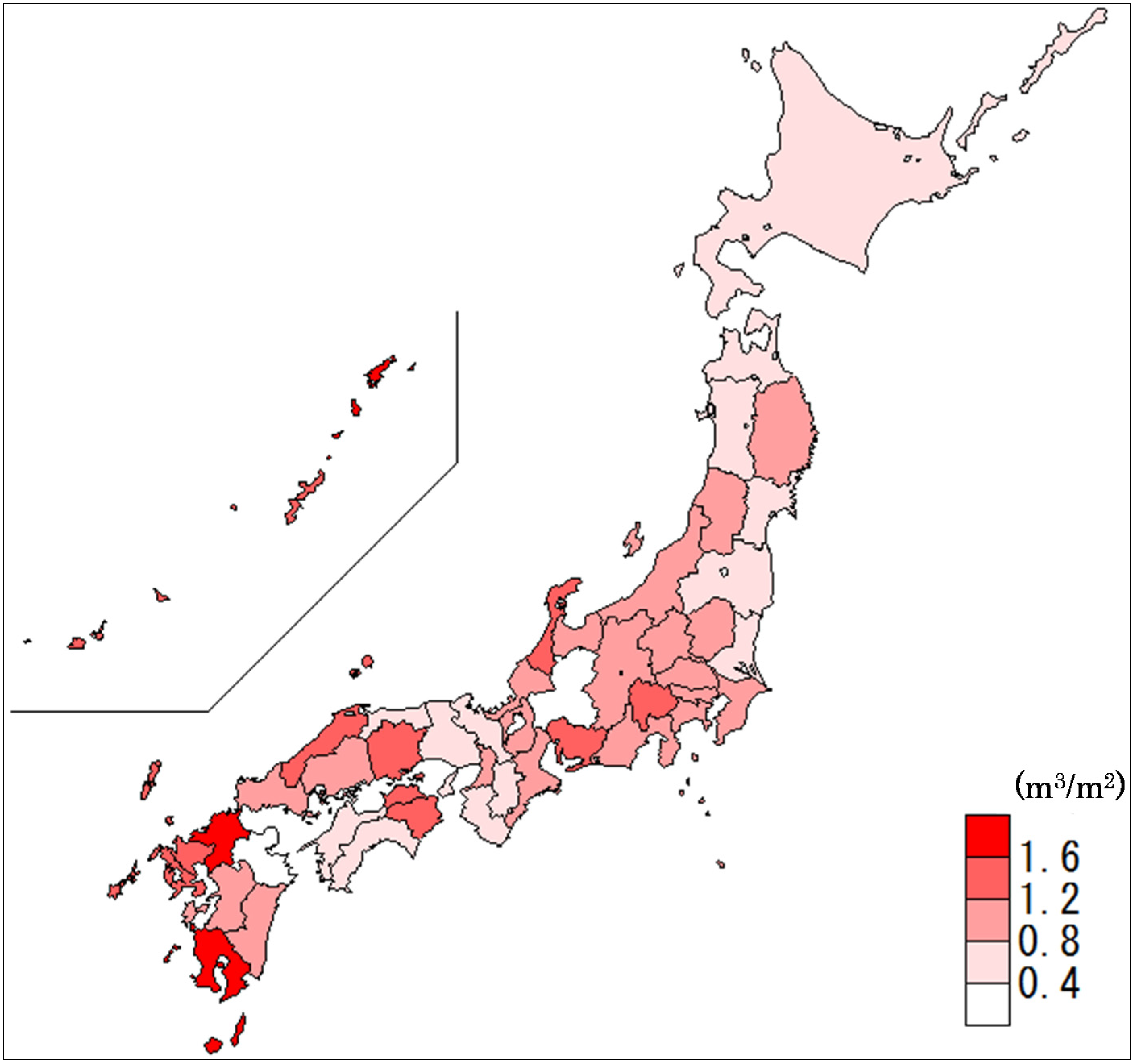
3.1. Intensity Factors of Availability Loss of Freshwater Attributed to Land Use

Table 2 shows average intensity factors of availability loss of freshwater by land use for all cells. Negative values in the table mean that the availability of freshwater increases with land-use change. Regarding paddy field and urban area, surplus flood flow on the ground owing to change of land cover recharges surface water to some extent, whereas a decrease of infiltration causes the loss of available groundwater. However, the net value of availability loss of water becomes positive. Both planted forest and arable land show no loss of available water in surface flow, because of high infiltration capacity (Table 1). The availability loss of freshwater in groundwater recharge shows a different tendency. For planted forest, the amount of evapotranspiration is greater than that of natural land, because the latter includes uncultivated land with a relatively small evapotranspiration ratio. This results in the small amount of availability loss in groundwater with planted forest. For arable land, the amount of evapotranspiration is lower than natural forest and the same as uncultivated land, which produced the negative value of availability loss in groundwater.
Table 2. Intensity factors of availability loss of freshwater attributable to land use.
Land Use TypeIntensity Factors of Availability Loss (m3/m2)
Surface FlowGroundwater Recharge
Planted forest03.87 × 10−4
Paddy field−0.2950.614
Arable land0−6.08 × 10⁻³
Urban area−0.5821.21
Urban area had the maximum net loss of freshwater availability caused by land use. The net intensity factor value for urban area was 0.629 m3/m2, representing ~37% of annual precipitation in Japan. This indicates that substantial freshwater input is lost by land-use change to urban area. The strength of land-use effects on freshwater availability presented spatial differences. Intensity factors for urban area aggregated into prefectural scale are depicted in Figure 3. Differences of intensity factors reached ~3.8 times, because of the disparity of precipitation and evapotranspiration. In addition to the regional differences of precipitation, evapotranspiration is determined by average daily temperature and average length of day that are also region-specific climate parameters. Depending on the balance of these three parameters, calculated intensity factors showed such differences. The lost amount of freshwater ranged from 6% to 117% of annual precipitation.
Figure 3. Intensity factors at prefectural scale attributed to urban area land use.
Sustainability 08 00086 g003

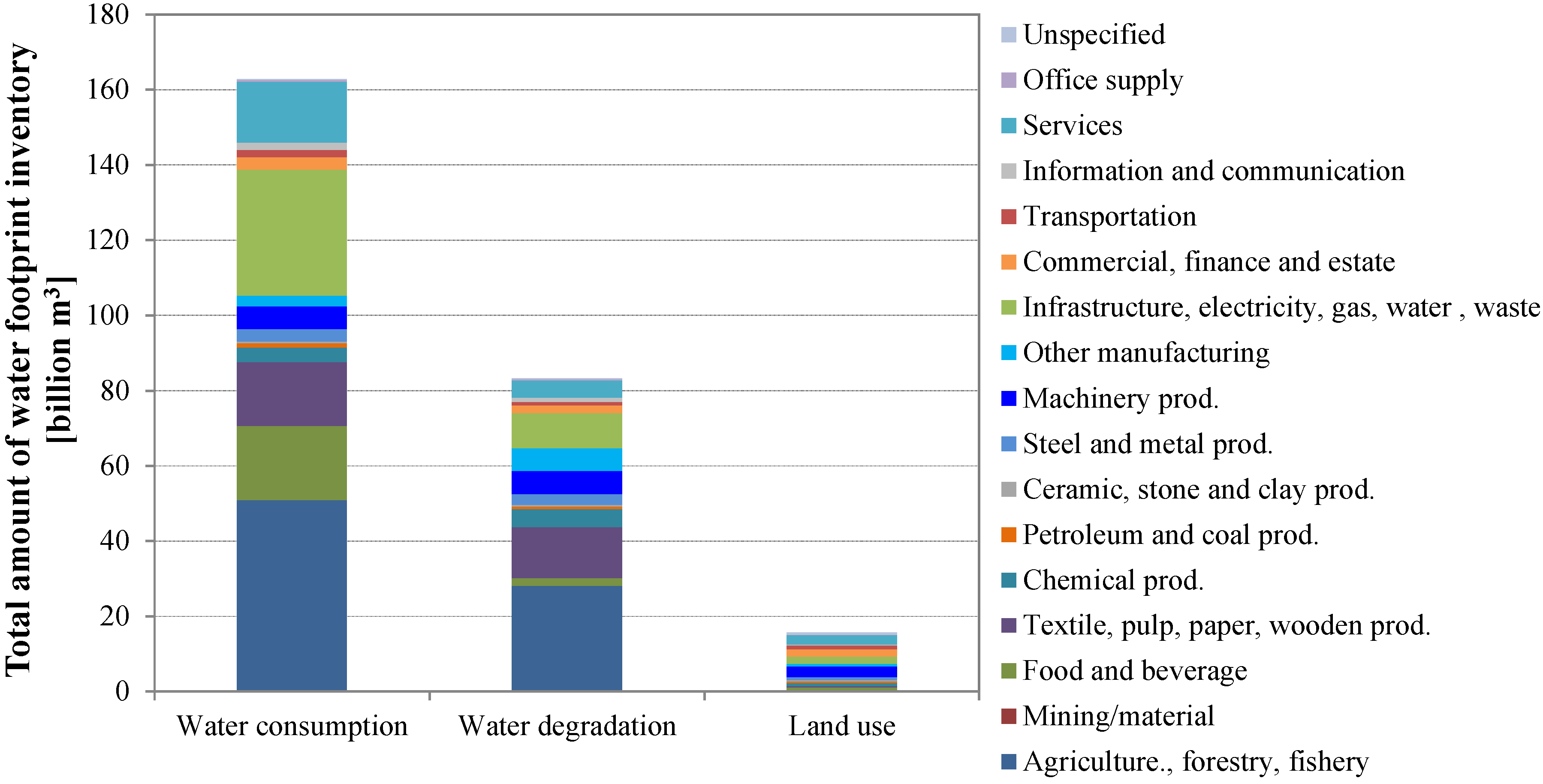
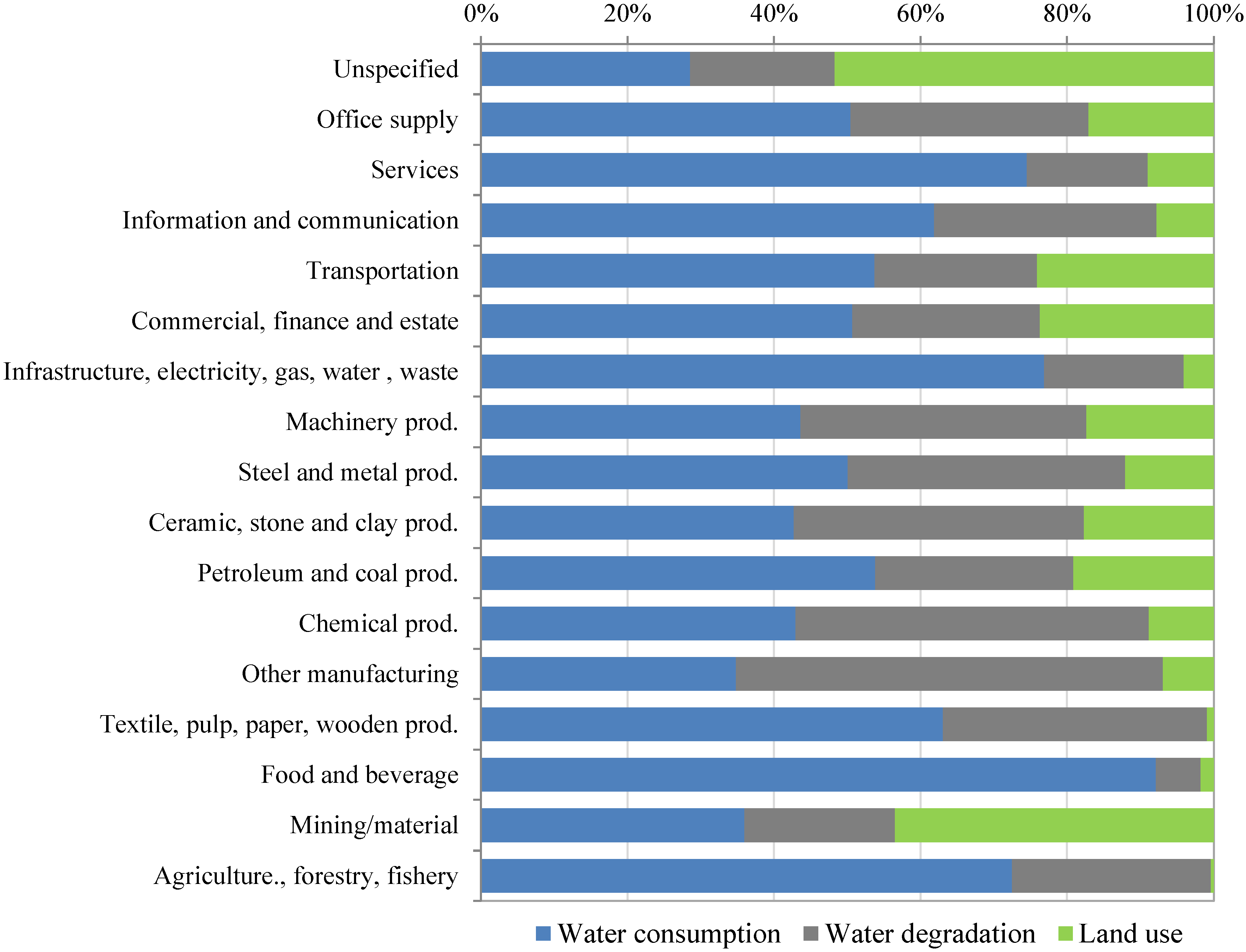
3.2. Water Footprint Inventory of Goods Produced in Japan

The total amount of water footprint inventory of all goods produced annually in Japan was calculated for water consumption, water degradation, and land use (Figure 4). The water footprint inventory of goods are aggregated in this figure into several sector categories that include similar goods. The largest water footprint inventory was from water consumption and was estimated at ~163 billion m3. The inventory related to water degradation was about half that of consumption (83 billion m3). Major categories with a large water footprint inventory showed some similarity in both cases. The total water footprint inventory related to land use was relatively small (~16 billion m3); around 10% of that was related to water consumption and 19% to water degradation. Unlike the cases of water consumption and degradation, secondary and tertiary sectors had a substantial water footprint inventory related to land use. Those two sectors generally occupy land as urban area with a greater intensity factor of freshwater availability loss as compared with planted forest, paddy fields, and arable land.
From a sectoral standpoint, the water footprint inventory for the three causes (water consumption, water degradation, and land use) was summarized, and proportions of each inventory to the summed inventory are shown in Figure 5. Although the absolute value of the inventory related to water consumption was the largest, the importance of each cause in the context of the inventory was sector-dependent. The categories “Agriculture, forestry, fishery” and “Infrastructure, electricity, gas, water, waste” show a dominance of water consumption and degradation in the water footprint inventory, because of heavy consumption by the agriculture and water supply sectors and strong emissions from the agriculture and water treatment sectors [26,27]. The same tendency was found for the categories “Food and beverage” and “Textile, pulp, paper, wooden production”, because agricultural products are used in those sectors. However, ~18% of the water footprint inventory on average (range 7%–51%) is attributed to land use in other sectors. This indicates that the effects of land use on the inventory are not negligible in comparison with water consumption and degradation in certain sectors.
Figure 4. Total amounts of water footprint inventory of Japanese goods.
Sustainability 08 00086 g004
Figure 5. Breakdown of total water footprint inventory for water consumption, water degradation, and land use for each sector category.
Sustainability 08 00086 g005

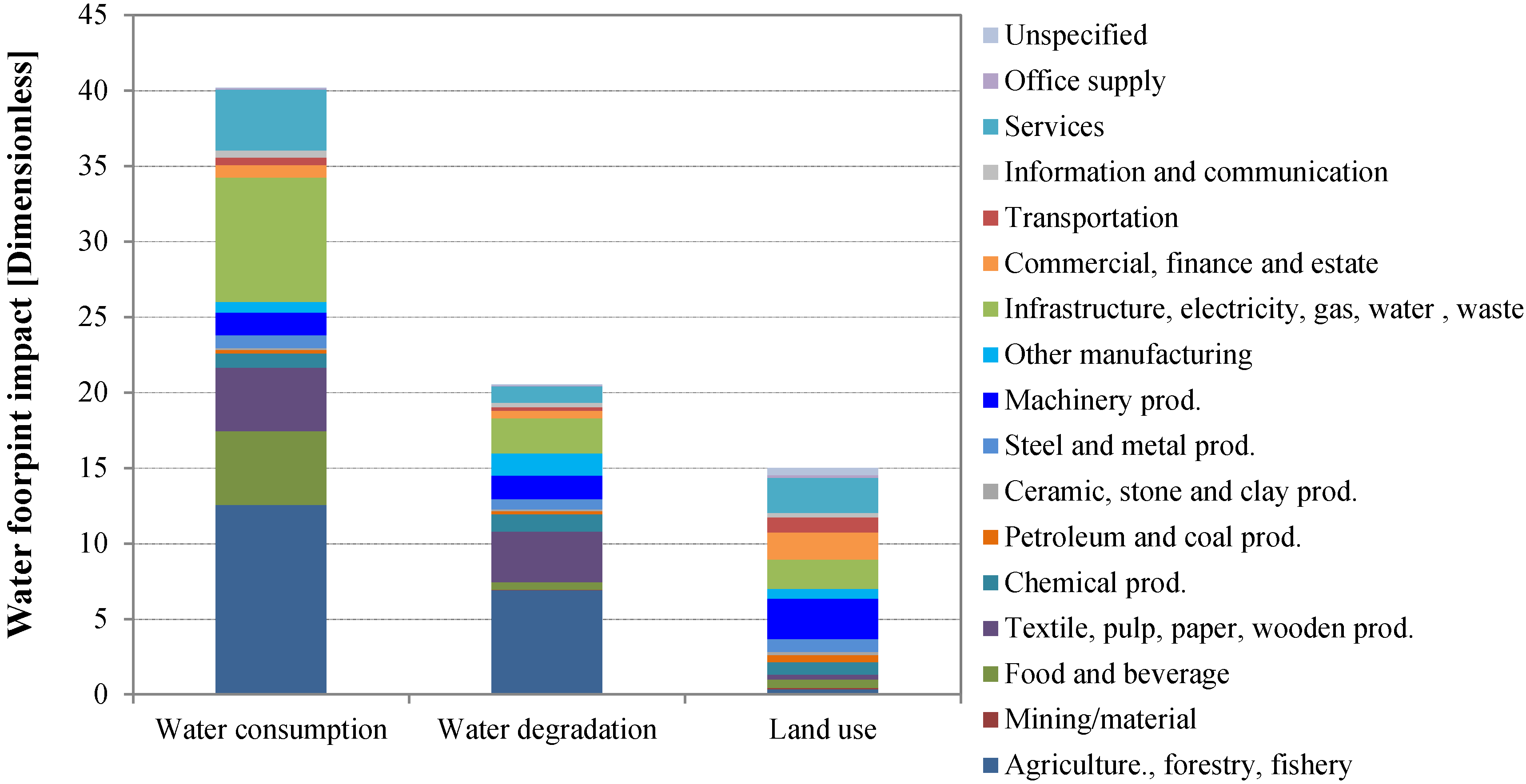
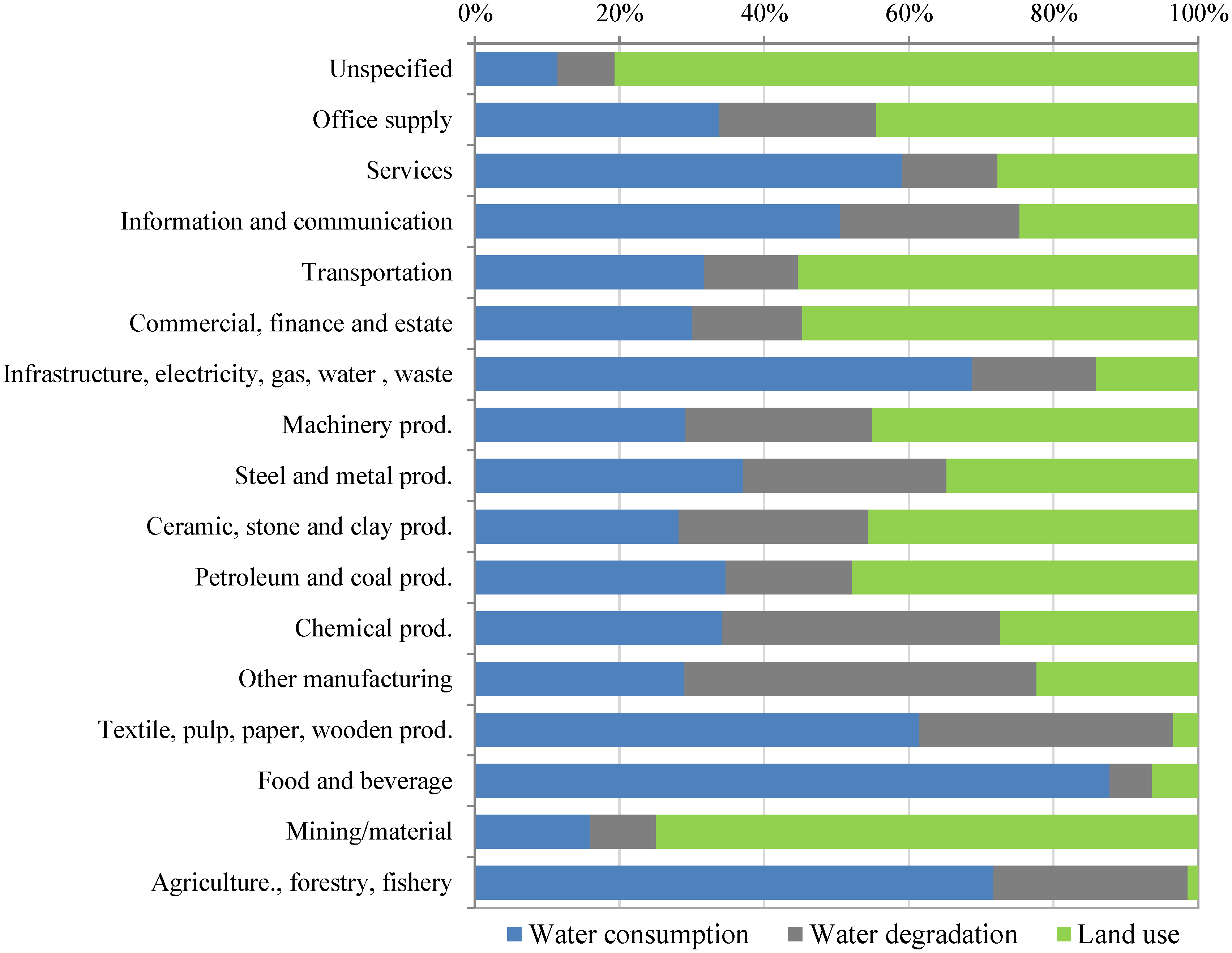
3.3. Water Footprint Impact of Goods Produced in Japan

Based on the calculated water footprint inventory and determined water scarcity index for surface water and groundwater (Section 2.5), the water footprint impact was assessed for the three causes in Figure 6. The relationship between water consumption and water degradation was not different from the water footprint inventory. However, the index value of water footprint impact for land use represents 37% of that for water consumption and 73% of that for water degradation. The importance of land use in the context of water footprint increases by considering the scarcity of various water resources. The dominance of land use in the water footprint impact was also stronger in many sectors than that in the water footprint inventory (Figure 7). If the effect of land use on freshwater availability was disregarded, there was an average underestimation of ~37% (range 0%–82%) in the water footprint impact assessment of goods produced in Japan.
Figure 6. Water footprint impacts of goods produced in Japan related to water consumption, water degradation, and land use.
Sustainability 08 00086 g006
Figure 7. Breakdown of total water footprint impacts for water consumption, water degradation, and land use for each sector category.
Sustainability 08 00086 g007

3.4. Sensitivity Analysis

The loss of freshwater availability due to land use was calculated as the difference of available freshwater amount in each land use type and natural land. For the definition of natural land, we assumed no change of the proportion of natural forest and uncultivated fields from the original situation as described in Section 2.2. Meanwhile, the balance of natural forest and uncultivated fields in each cell showed distribution (Figure 8). While there is no robust evidence of the original situation, this variance may affect the results of intensity factor calculation of freshwater availability loss caused by land use. Sensitivity of intensity factor with the variance of the ratio of natural forest area to total natural land (natural forest + uncultivated fields) was analyzed. According to the 90% confidential interval, the threshold values of the ratio of natural forest area to total natural land were determined as 0.113 for the lower 5% and 1 for the higher 5% and used as the edges for sensitivity analysis.
Figure 8. Distribution of ratio of forest in natural land with cumulative percentage of cells.
Sustainability 08 00086 g008
Regarding paddy field and urban area, the coefficient of variation (CV) resulted in around 0.282–0.348 for both of surface flow and groundwater recharge (Table 3). This meant that intensity factors of availability loss ranged within ±28.2%–34.8% from average values in most cases (statistically about 68.3%). On the other hand, CVs in the case of planted forest and arable land were calculated for groundwater recharge as 1.21 (planted forest) and 1.02 (arable land), respectively (Table 3). This indicated that variation of intensity factors of availability loss changed around ±102%–121% from average values in most cases of planted forest and arable land. As shown in Table 1, planted forest and arable land have high infiltration capacity similarly to natural land (natural forest and uncultivated land). Meanwhile, natural forest and planted forest have higher evapotranspiration ratios than uncultivated land and arable land. This resulted in the net increase of groundwater recharge in arable land use and the net decrease of that in planted forest even though arable land had relatively lower infiltration capacity than natural and planted forest (Table 2). Therefore, the ratio of natural forest affects the amount of groundwater recharge in natural land as a result of high evapotranspiration capacity. This caused high sensitivity of intensity factors of availability loss in groundwater recharge, especially in the case of planted forest and arable land that have relatively higher groundwater recharge ability. Infiltration capacity of paddy field and urban area is rather lower than arable land (Table 1), which results in relatively large intensity factor of availability loss in ground water recharge (Table 2). Thus, the effect of natural forest ratio in natural land caused lower sensitivity in paddy field and urban area.
Table 3. Results of sensitivity analysis: average values calculated based on current situation and coefficient of variation based on variant natural forest ratio in natural land.
Land Use TypeIntensity Factors of Availability Loss (m3/m2)
Surface FlowGroundwater Recharge
AverageCoefficient of VariationAverageCoefficient of Variation
Planted forest03.87 × 10−41.21
Paddy field−0.2950.3470.6140.348
Arable land0−6.08 × 10−31.02
Urban area−0.5820.2821.210.284

4. Conclusions

The nexus between water availability and land use has not been analyzed and discussed in detail within prior studies of water footprinting. Water balance model calculation quantitatively reveals that land cover change attributed to artificial land use may cause loss of freshwater availability in surface and groundwater by affecting surface flow and groundwater recharge. The net loss of available freshwater is ~37% of annual water input by precipitation, with wide variation due to local climate conditions. Thus, the effect of artificial land use related to production activities must be considered in the assessment of the water footprint of goods.
From the viewpoint of water footprint inventory, water consumption is responsible for a large part of the total water footprint inventory related to water consumption, water degradation, and land use. However, the water footprint effect of goods considering scarcity of various freshwater sources emphasizes the significance of land use in the context of assessing all effects relevant to water. Meanwhile, intensity factor of availability loss may change ±28.2%–121% from average in most cases (around 68.3%) depending on the definition of natural land as a base line.
Although spatial differences of land use effects were found by water balance analysis at grid scale, the inventory of water consumption, pollution emission, and land area used in our study does not specify location. Identification of spatial information on water consumption, water degradation, and land use is not easy because enormous time and effort is required. However, improvement of spatial resolution in the water footprint assessment would describe the importance of the nexus between water and land use more precisely. The temporal resolution in the present study was one year. It is obvious that freshwater demand is not constant with time but seasonal, especially for agricultural users. The importance of temporal variation has been pointed out [30]. Spatial and temporal resolution must be improved in future studies.

Acknowledgments

This work was partly supported by Grant-in-Aid for Young Scientists (A) (JSPS KAKENHI 15H05342).

Author Contributions

All authors contributed equally to all parts of the research, in the analysis, data interpretation, and manuscript writing and editing. All authors have read and approved the final manuscript.

Conflicts of Interest

The authors declare no conflict of interest.

References

  1. Shiklomanov, I.A.; Rodda, J.C. World Water Resources at the Beginning of the Twenty-First Century; Cambridge University Press: Cambridge, UK, 2003. Available online: http://catdir.loc.gov/catdir/samples/cam034/2002031201.pdf (accessed on 15 October 2015).
  2. The International Organization for Standardization. Environmental Management—Water Footprint—Principles, Requirements and Guidelines; ISO14046; International Organization for Standardization: Geneva, Switzerland, 2014. [Google Scholar]
  3. Kounina, A.; Margni, M.; Bayart, J.B.; Boulay, A.M.; Berger, M.; Bulle, C.; Frischknecht, R.; Koehler, A.; Milà i Canals, L.; Motoshita, M.; et al. Review of methods addressing freshwater use in life cycle inventory and impact assessment. Int. J. Life Cycle Assess. 2013, 18, 707–721. [Google Scholar] [CrossRef]
  4. Boulay, A.M.; Bare, J.; Camillis, C.D.; Döll, P.; Gassert, F.; Gerten, D.; Humbert, S.; Inaba, A.; Itsubo, N.; Lemoine, Y.; et al. Consensus building on the development of a stress-based indicator for LCA-based impact assessment of water consumption: Outcome of the expert workshops. Int. J. Life Cycle Assess. 2015, 20, 577–583. [Google Scholar] [CrossRef]
  5. European Commission—Joint Research Centre—Institute for Environment and Sustainability. International Reference Life Cycle Data System (ILCD) Handbook—Framework and Requirements for Life Cycle Impact Assessment Models and Indicators, 1st ed.; Publication Office of the European Union: Luxembourg, 2010; p. 103. [Google Scholar]
  6. Verones, P.; Saner, D.; Pfister, S.; Baisero, D.; Rondinini, C.; Hellweg, S. Effects of consumptive water use on wetlands of international importance. Environ. Sci. Technol. 2013, 747, 12248–12257. [Google Scholar] [CrossRef] [PubMed]
  7. Pfister, S.; Suh, S. Environmental impacts of thermal emissions to freshwater: Spatially explicit fate and effect modeling for life cycle assessment and water footprinting. Int. J. Life Cycle Assess. 2015, 20, 927–936. [Google Scholar] [CrossRef]
  8. Quinteiro, P.; Dias, A.C.; Araújo, A.; Pestana, J.L.T.; Ridoutt, B.G.; Arroja, L. Suspended solids in freshwater systems: Characterization model describing potential impacts on aquatic biota. Int. J. Life Cycle Assess. 2015, 20, 1232–1242. [Google Scholar] [CrossRef]
  9. Hoekstra, A.Y.; Chapagain, A.K.; Aldaya, M.M.; Mekonnen, M.M. The Water Footprint Assessment Manual: Setting the Global Standard; Earthscan: London, UK, 2011; p. 197. [Google Scholar]
  10. Fehrenbach, H.; Grahl, B.; Giegrich, J.; Busch, M. Hemeroby as an impact category indicator for the integration of land use into life cycle (impact) assessment. Int. J. Life Cycle Assess. 2015. [Google Scholar] [CrossRef]
  11. Ridoutt, B.G.; Juliano, P.; Sanguansri, P.; Sellahewa, J. The water footprint of food waste: Case study of fresh mango in Australia. J. Clean. Prod. 2010, 18, 1714–1721. [Google Scholar] [CrossRef]
  12. Núñez, M.; Pfister, S.; Roux, P.; Antón, A. Estimating water consumption of potential natural vegetation on global dry lands: Building an LCA framework for green water flows. Environ. Sci. Technol. 2013, 47, 12258–12265. [Google Scholar] [CrossRef] [PubMed]
  13. Quinteiro, P.; Dias, A.C.; Silva, M.; Ridoutt, B.G.; Arroja, L. A contribution to the environmental impact assessment of green water flows. J. Clean. Prod. 2015, 93, 318–329. [Google Scholar] [CrossRef]
  14. Milà i Canals, L.; Chenoweth, J.; Chapagain, A.; Orr, S.; Antón, A.; Clift, R. Assessing freshwater use impacts in LCA: Part I—Inventory modelling and characterisation factors for the main impact pathways. Int. J. Life Cycle Assess. 2009, 14, 28–42. [Google Scholar] [CrossRef]
  15. National Land Information Division, National Spatial Planning and Regional Policy Bureau, Ministry of Land, Infrastructure, Transport and Tourism, National Land Numerical Information Download Service. Available online: http://nlftp.mlit.go.jp/ksj-e/index.html (accessed on 4 January 2012).
  16. Thornthwaite, C.W. An approach toward a rational classification of climate. Geogr. Rev. 1948, 38, 55–94. [Google Scholar] [CrossRef]
  17. Forestry Agency, Current Status of Forestry Resources, The Ministry of Agriculture, Forestry and Fisheries (MAFF) Web. Available online: http://www.rinya.maff.go.jp/j/keikaku/genkyou/h24/3.html (accessed on 10 October 2015).
  18. Tsukamoto, Y. Forestry Hydrology; Buneido: Tokyo, Japan, 1992; ISBN 978-4-8300-4058-0. (In Japanese) [Google Scholar]
  19. Pidwirny, M. The Hydrologic Cycle. Fundamentals of Physical Geography, 2nd ed. Available online: http://www.physicalgeography.net/fundamentals/8b.html (accessed on 10 October 2015).
  20. Tosaki, Y.; Tase, N.; Sasa, K.; Takahashi, T.; Nagashima, Y. Estimation of groundwater residence time using the 36Cl bomb pulse. Groundwater 2011, 49, 891–902. [Google Scholar] [CrossRef] [PubMed] [Green Version]
  21. Kashiwaya, K.; Hasegawa, T.; Nakata, K.; Tomioka, Y.; Mizuno, T. Multiple tracer study in Horonobe, northern Hokkaido, Japan: 1. Residence time estimation based on multiple environmental tracers and lumped parameter models. J. Hydrol. 2014, 519, 532–548. [Google Scholar] [CrossRef]
  22. Sakaguchi, A.; Ohtsuka, Y.; Yokota, K.; Sasaki, K.; Komura, K.; Yamamoto, M. Cosmogenic radionuclide 22Na in the Lake Biwa system (Japan): Residence time, transport and application to the hydrology. Earth Planet. Sci. Lett. 2005, 231, 307–316. [Google Scholar] [CrossRef]
  23. Current State of Water Resources in Japan. The Ministry of Land, Infrastructure, Transport and Tourism (MLIT) Web. Available online: http://www.mlit.go.jp/tochimizushigen/mizsei/water_resources/contents/current_state.html (accessed on 10 October 2015).
  24. Rates of Sources for Agricultural Withdrawal of Water. The Ministry of Agriculture, Forestry and Fisheries (MAFF) Web. Available online: http://www.maff.go.jp/j/council/seisaku/nousin/bukai/h24_4/pdf/data1-2_4.pdf (accessed on12 October 2015). (In Japanese)
  25. Japan Water Works Association. Water Supply in Japan 2014. Available online: http://www.jwwa.or.jp/jigyou/kaigai_file/2014WaterSupplyInJapan.pdf (accessed on 12 October 2015).
  26. Ono, Y.; Motoshita, M.; Itsubo, N. Development of water footprint inventory database on Japanese goods and services distinguishing the types of water resources and the forms of water uses based on input-output analysis. Int. J. Life Cycle Assess. 2015, 20, 1456–1467. [Google Scholar] [CrossRef]
  27. Ono, Y.; Motoshita, M.; Itsubo, N. Development of water footprint inventory database considering pollution. J. Life Cycle Assess. Jpn. 2015, 11, 22–31. (In Japanese) [Google Scholar] [CrossRef]
  28. Horiguchi, K.; Itsubo, N. Development of land use inventory using input-output analysis for life cycle assessment. Pap. Environ. Inf. Sci. 2011, 25, 19–24. (In Japanese) [Google Scholar]
  29. FAO, AQUASTAT. Food and Agriculture Organization of United Nations Web. Available online: http://www.fao.org/nr/water/aquastat/main/index.stm (accessed on 7 September 2010).
  30. Pfister, S.; Bayer, P. Monthly water stress: Spatially and temporally explicit consumptive water footprint of global crop production. J. Clean. Prod. 2014, 73, 53–62. [Google Scholar] [CrossRef]

