Author Contributions
Conceptualization, F.D.; methodology, F.D.; software, F.D.; validation, F.D., B.L. and H.R.; formal analysis, F.D.; investigation, F.D.; data curation, F.D.; writing—original draft preparation, F.D.; writing—review and editing, F.D., B.L. and H.R.; visualization, F.D.; supervision, B.L. and H.R. All authors have read and agreed to the published version of the manuscript.
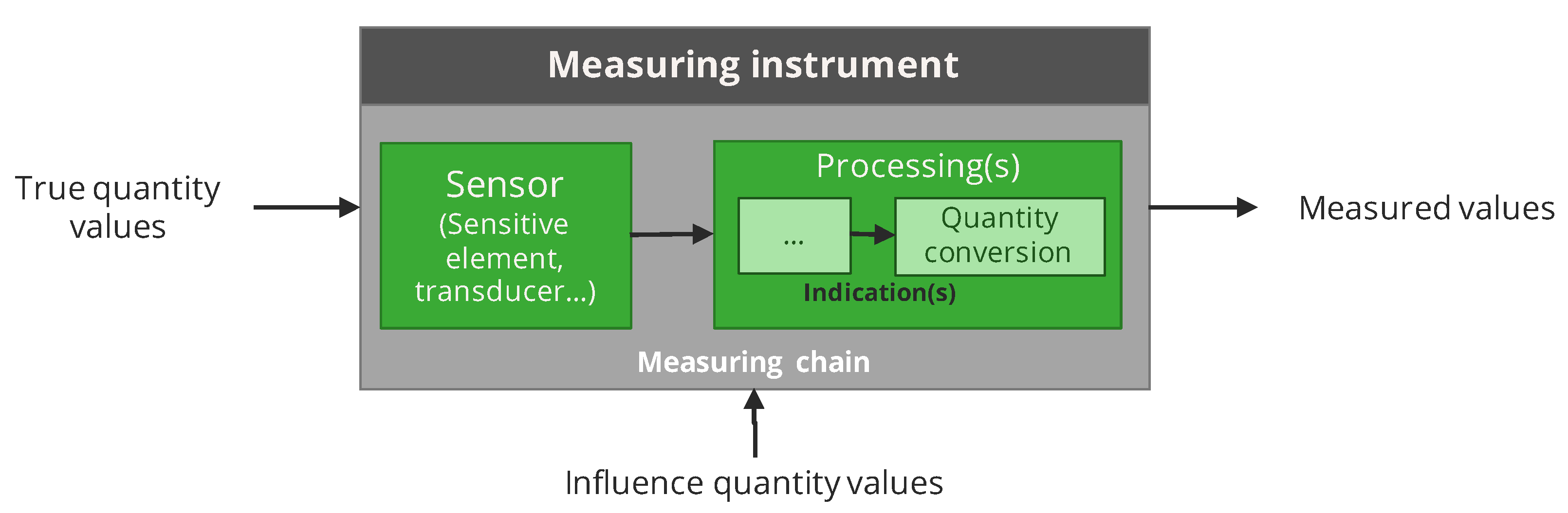
Figure 1.
Model adopted for the measuring instruments. It is considered as a grey box, for example, an algorithm mimics the behaviour of the components of the measuring chain without however modelling each part individually.
Figure 1.
Model adopted for the measuring instruments. It is considered as a grey box, for example, an algorithm mimics the behaviour of the components of the measuring chain without however modelling each part individually.
Figure 2.
Schematic diagram of the methodology proposed for in situ calibration strategies evaluation.
Figure 2.
Schematic diagram of the methodology proposed for in situ calibration strategies evaluation.
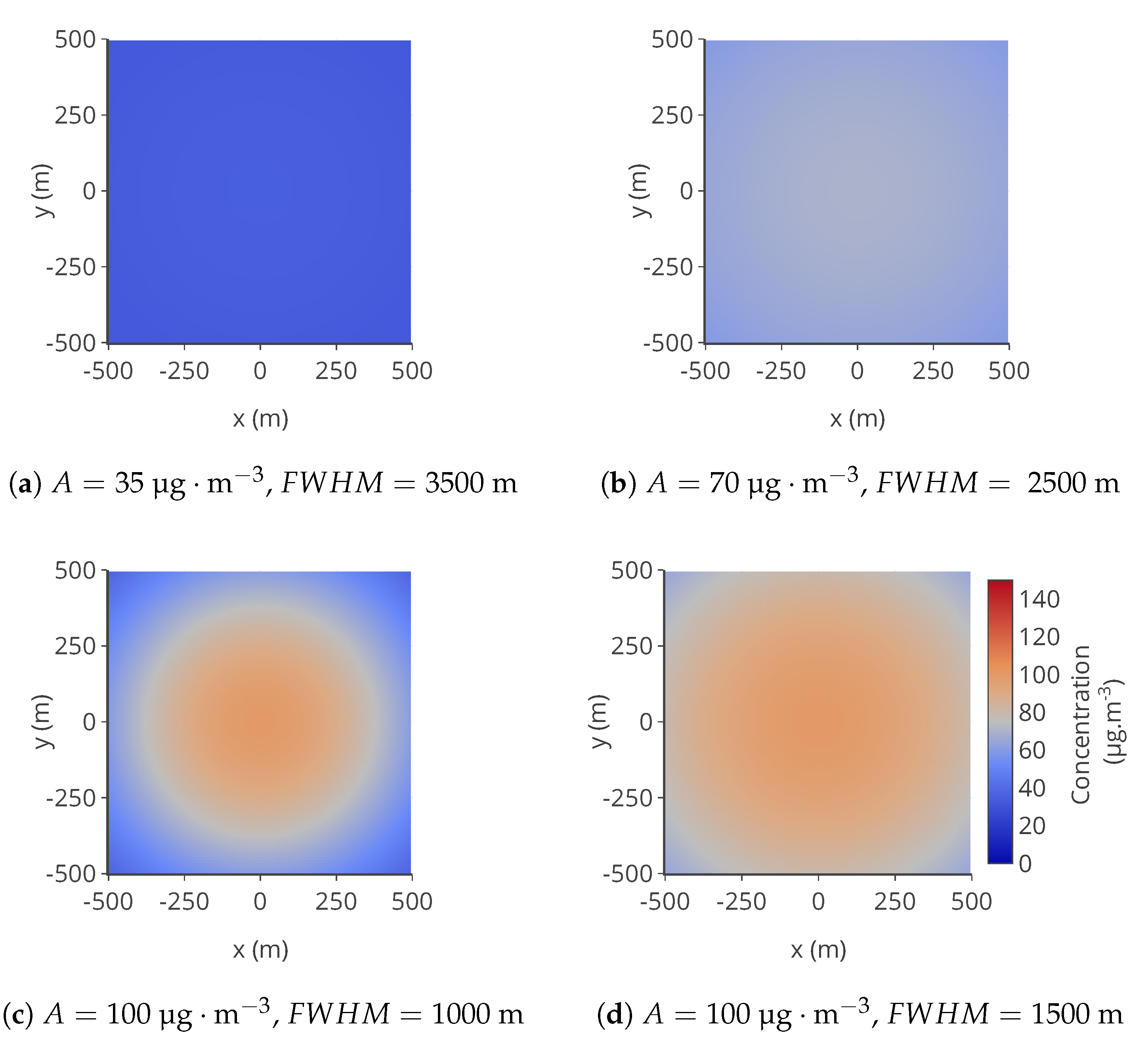
Figure 3.
Examples of maps of concentration C used following for given A and .
Figure 3.
Examples of maps of concentration C used following for given A and .
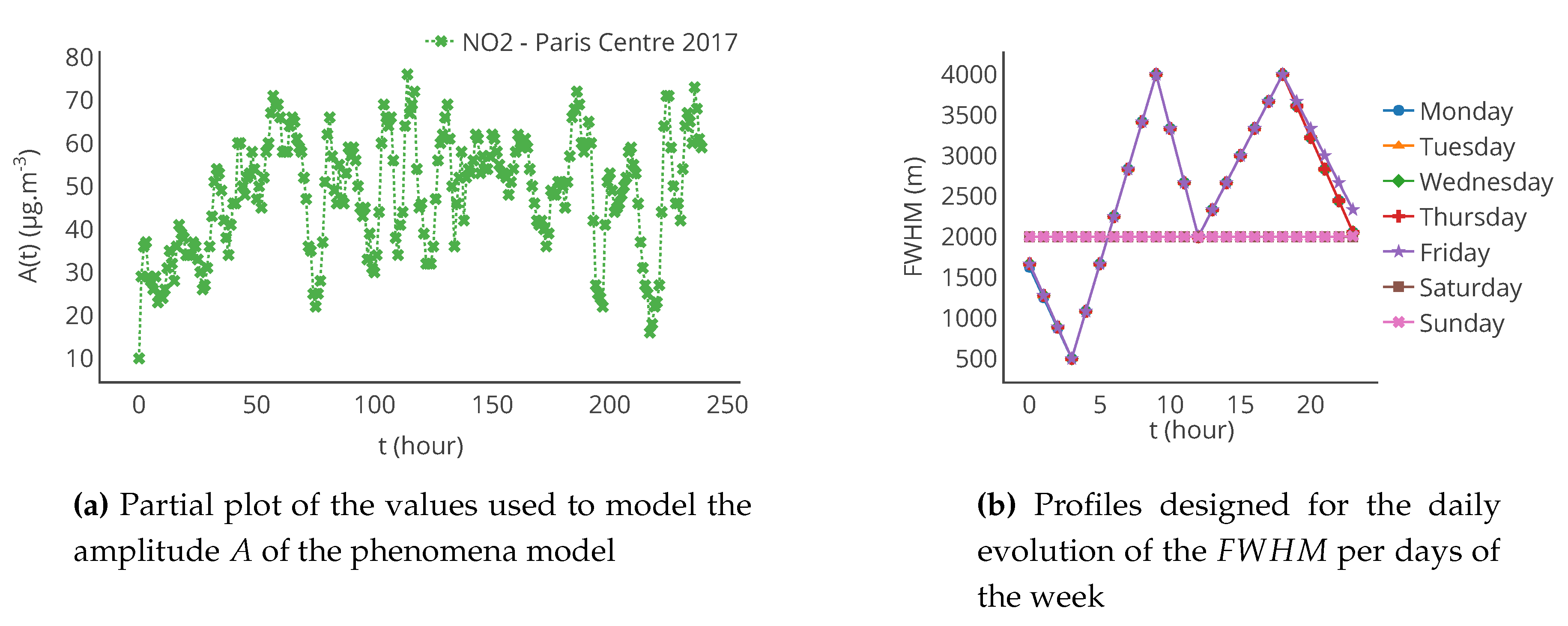
Figure 4.
Evolution of A and for the modelling of the concentration of pollutant.
Figure 4.
Evolution of A and for the modelling of the concentration of pollutant.
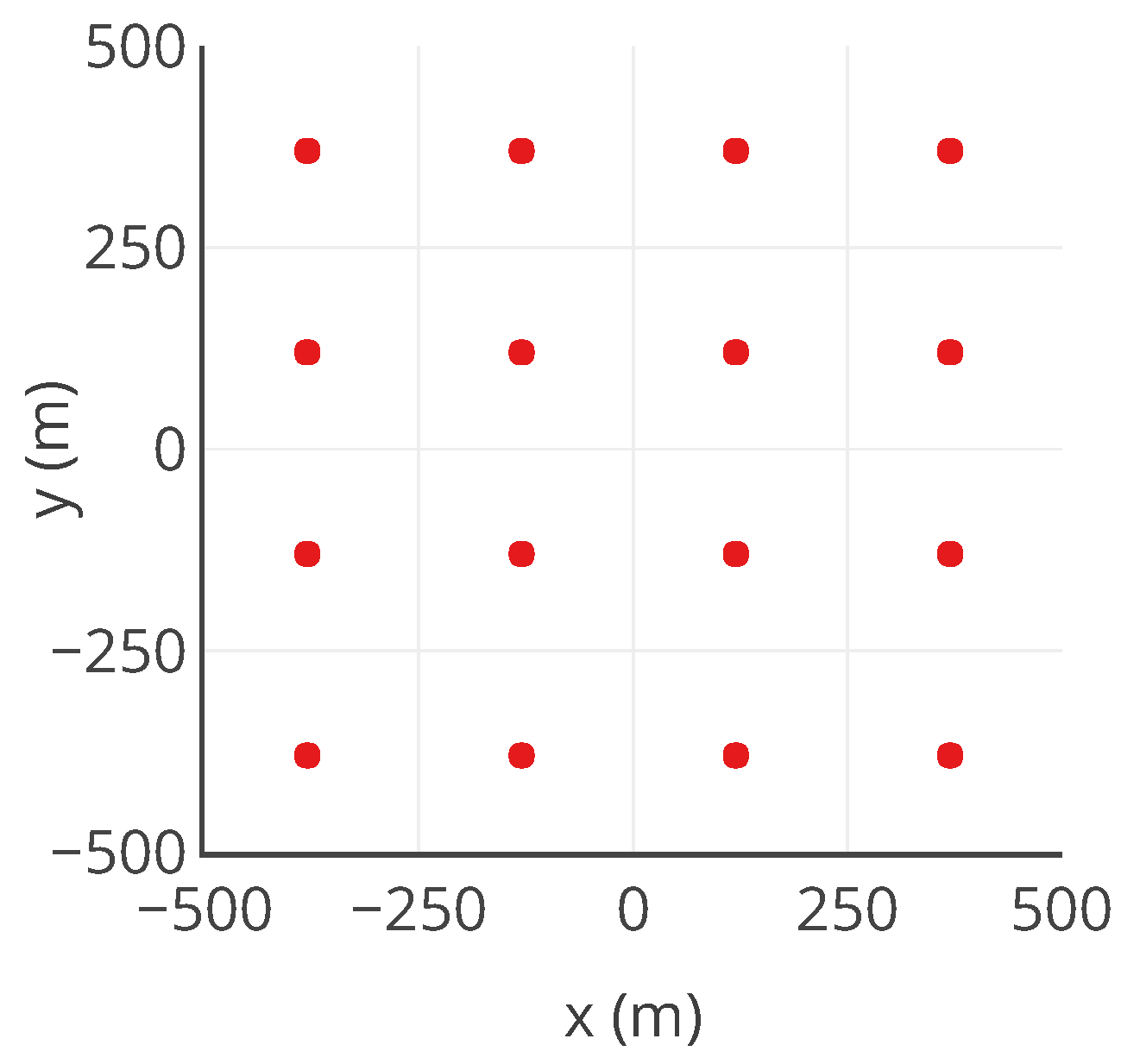
Figure 5.
Positions of the 16 sensors considered in the case study, deployed uniformly in the field.
Figure 5.
Positions of the 16 sensors considered in the case study, deployed uniformly in the field.
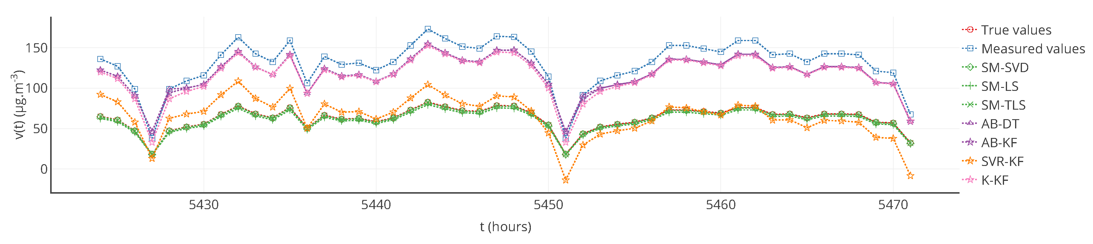
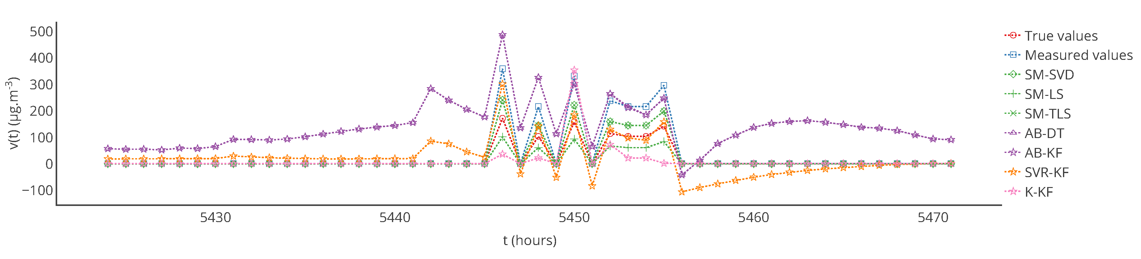
Figure 6.
True values, measured values and corrected values with the strategies considered for a particular sensor between and . SM-(SVD, LS, TLS) and SVR-KF seem to provide better results than AB-DT, AB-KF and K-KF.
Figure 6.
True values, measured values and corrected values with the strategies considered for a particular sensor between and . SM-(SVD, LS, TLS) and SVR-KF seem to provide better results than AB-DT, AB-KF and K-KF.
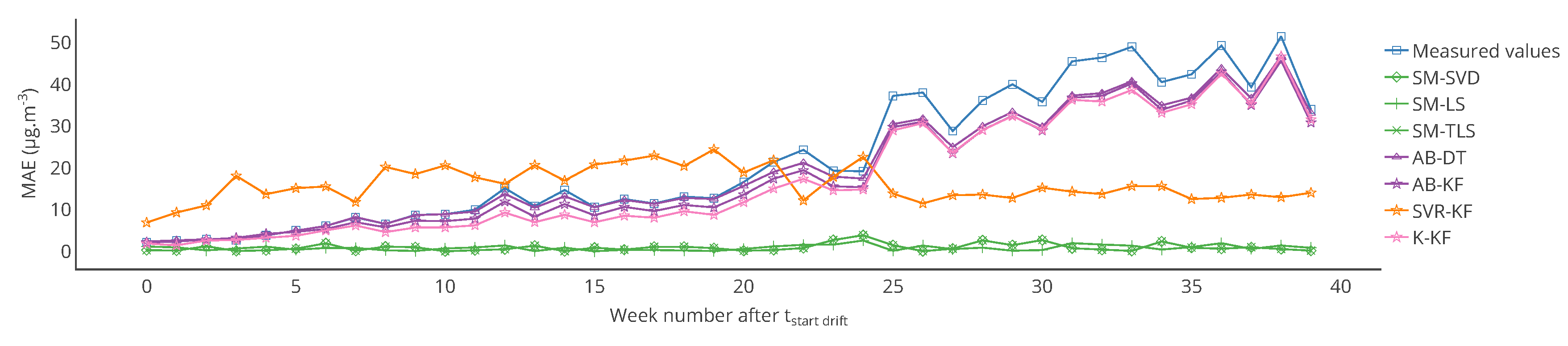
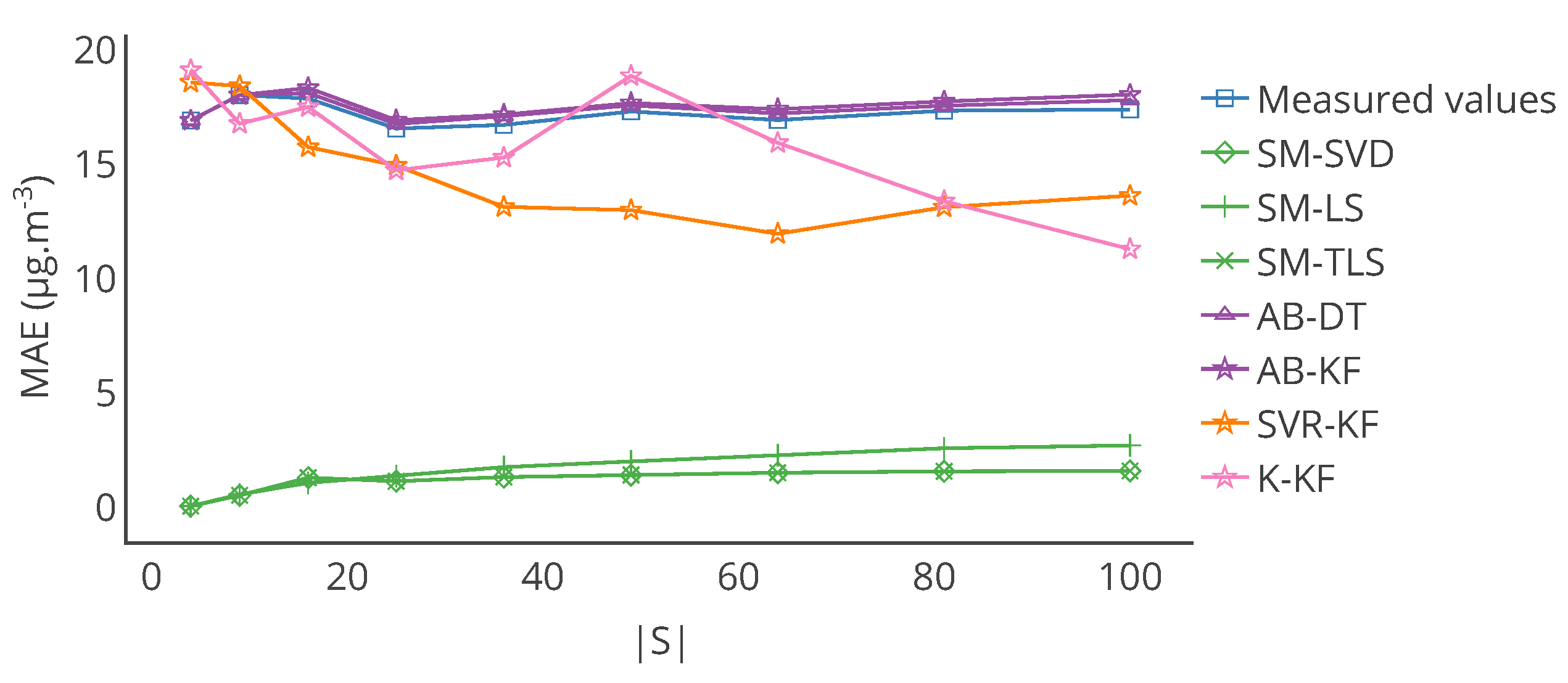
Figure 7.
Evolution of the MAE computed for each week of the drift period between the drifted values and the true values, and between the corrected values for each strategy and the true values for a particular sensor, after the start of drift. MAE for SVR-KF is nearly always worse than those for AB-DT, AB-KF and K-KF until week 24 but are better afterwards. The performances of SVR-KF could be explained by the presence of a bias, at least according to this metrics, as its evolution is quite flat.
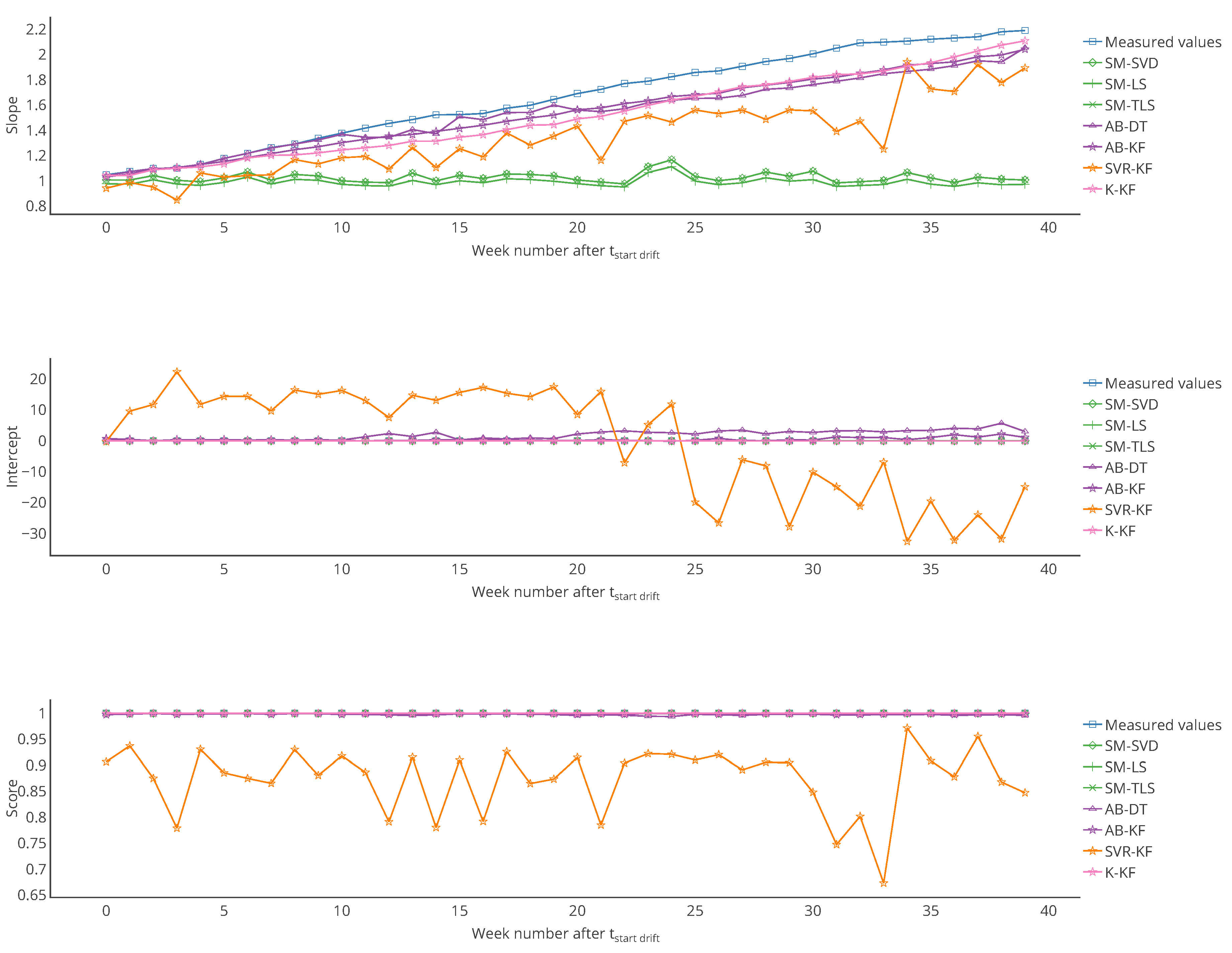
Figure 8.
Evolution of the slope, intercept and score of the error model of , computed on each week of the drift period. From these figures we observe that both the slope and intercept are locally poor for SVR-KF, although this is not visible when computing the error model on the entire time interval of study. This explains the poor values of the score for this algorithm. Regarding the other strategies, the intercept and score are quite constant. The slope is also quite constant for SM-(SVD, LS, TLS) but it mainly follows the evolution the slope of the measured valued for AB-(DT, KF) and K-KF.
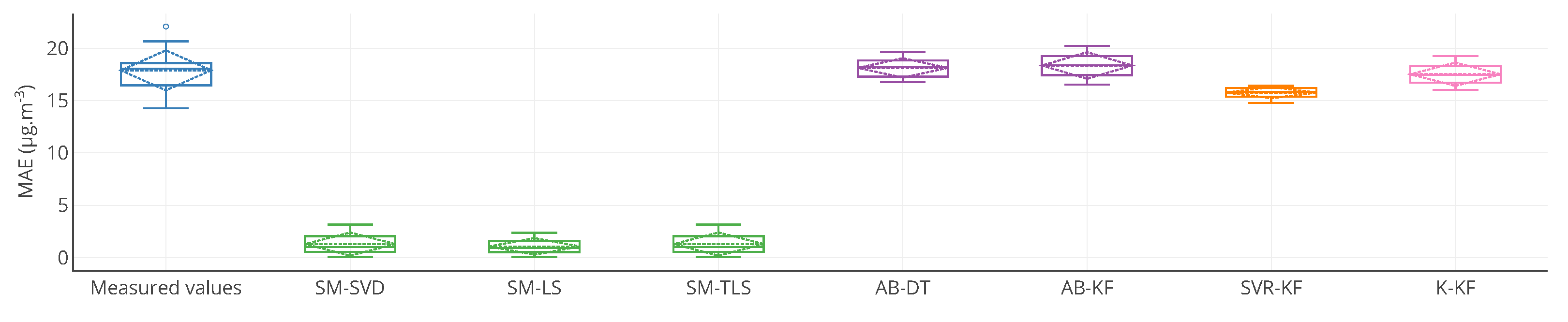
Figure 9.
Box plots of the MAE, computed on the entire time interval of drift, of the 16 nodes of the network without calibration and with SM-SVD. It is a graphical representation of the information displayed in
Table 1 for MAE.
Supplementary information is provided compared to the table: quartiles, minimum and maximal values.
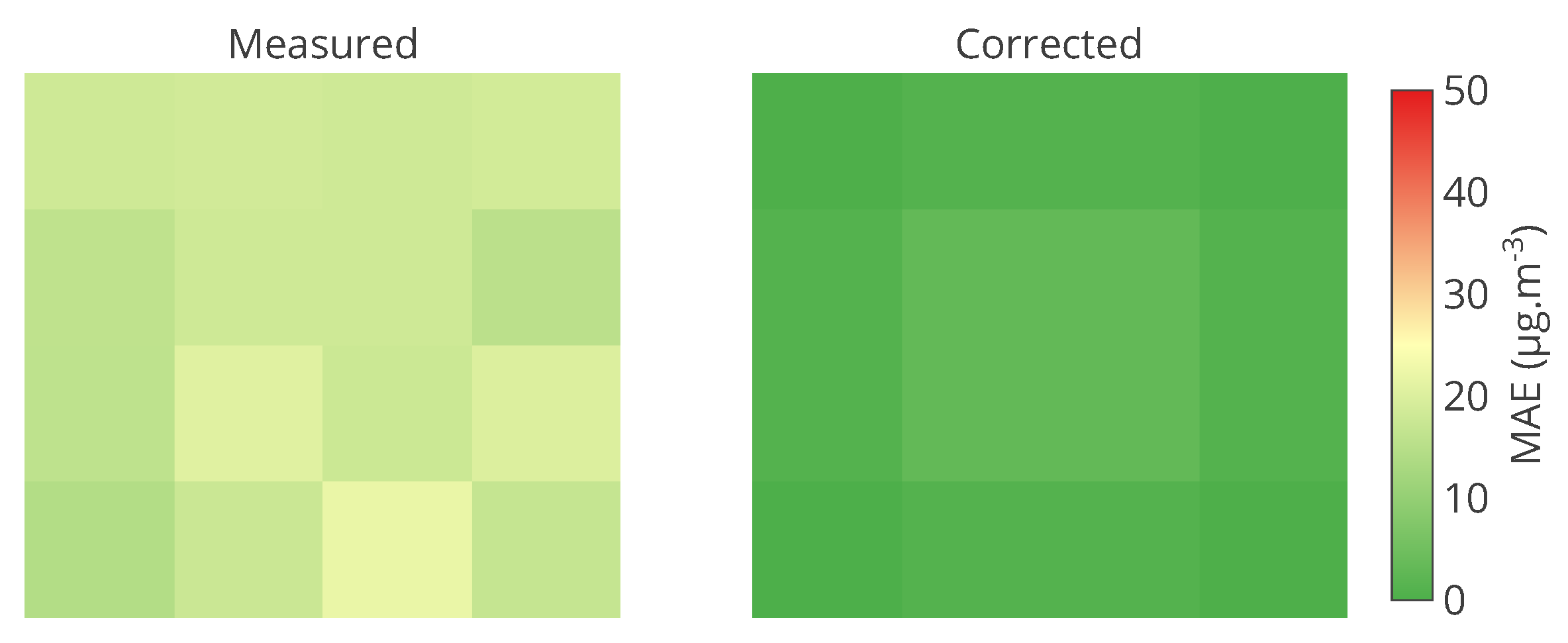
Figure 10.
Matrix of the MAE, computed on the entire time interval of drift, of the 16 nodes of the network without calibration and with SM-SVD. It shows exactly the information for each instrument. The colour scale can help to identify problematic instruments.
Figure 10.
Matrix of the MAE, computed on the entire time interval of drift, of the 16 nodes of the network without calibration and with SM-SVD. It shows exactly the information for each instrument. The colour scale can help to identify problematic instruments.
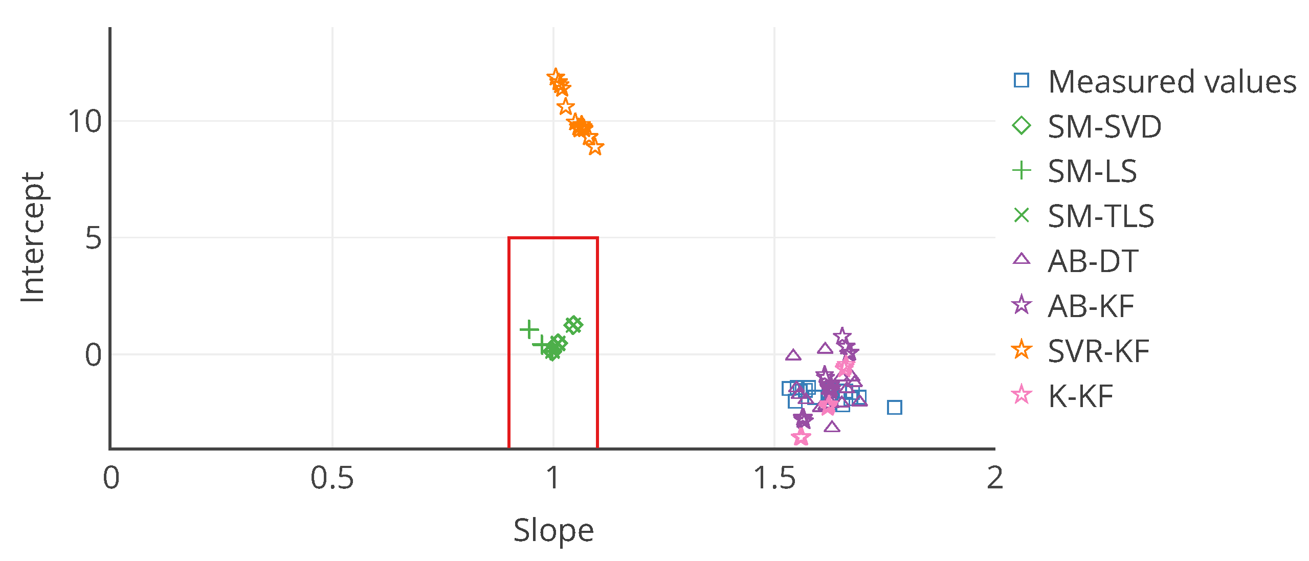
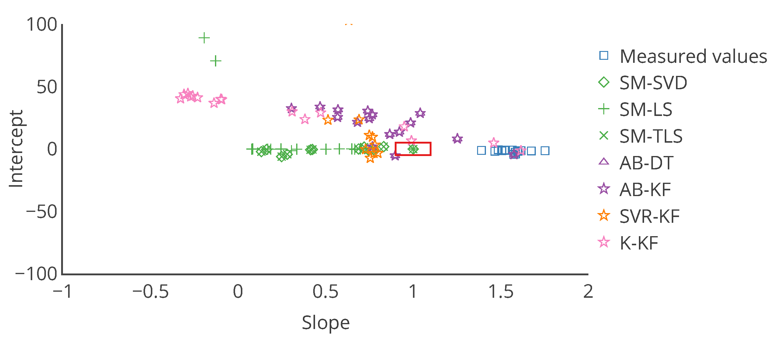
Figure 11.
Target plot of the 16 nodes as a function of their slope and intercept in the error model for each calibration strategy. The slope and intercept are computed on the entire time interval of drift. In this case, it allows to locate an instrument according to the slope and intercept of its associated error model. The red rectangle is an example of area that can be defined to quickly identify instruments that are not satisfying a requirement, here a slope in and an intercept in .
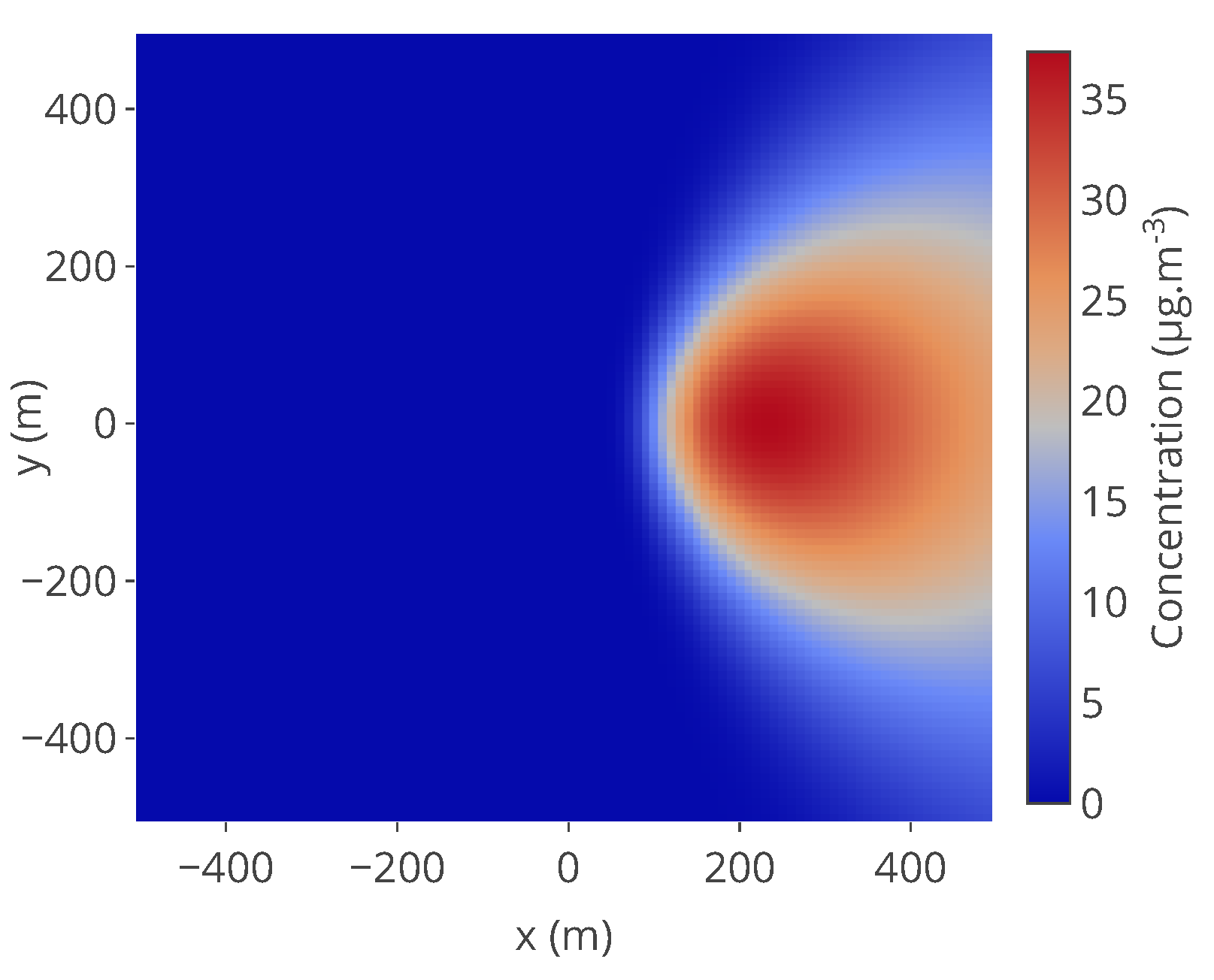
Figure 12.
Example of concentration map used and based on the Gaussian plume model. The pollutant source is at coordinates , , the map is observed at . The other parameters are: {T = 25 °C, Vw = 10 m s−1, Ts = 30 °C, g = 9.8 m s−2, D = 1.9 × 10⁻⁹ m3 s−1, Q = 5 × 10⁻³ kg s−1, σy = 1.36|x−xs|0.82, σz = 0.275|x−xs|0.69}. Wind direction is equal to 0° here.
Figure 13.
True values, measured values and corrected values with the strategies considered for a particular sensor between
and
with the Gaussian plume model. Note that the profiles of the curves are very different from those of
Figure 6 as instruments are not necessarily exposed to the plume of pollutant due to the wind direction. In this case it is exposed to the pollutant between
and
.
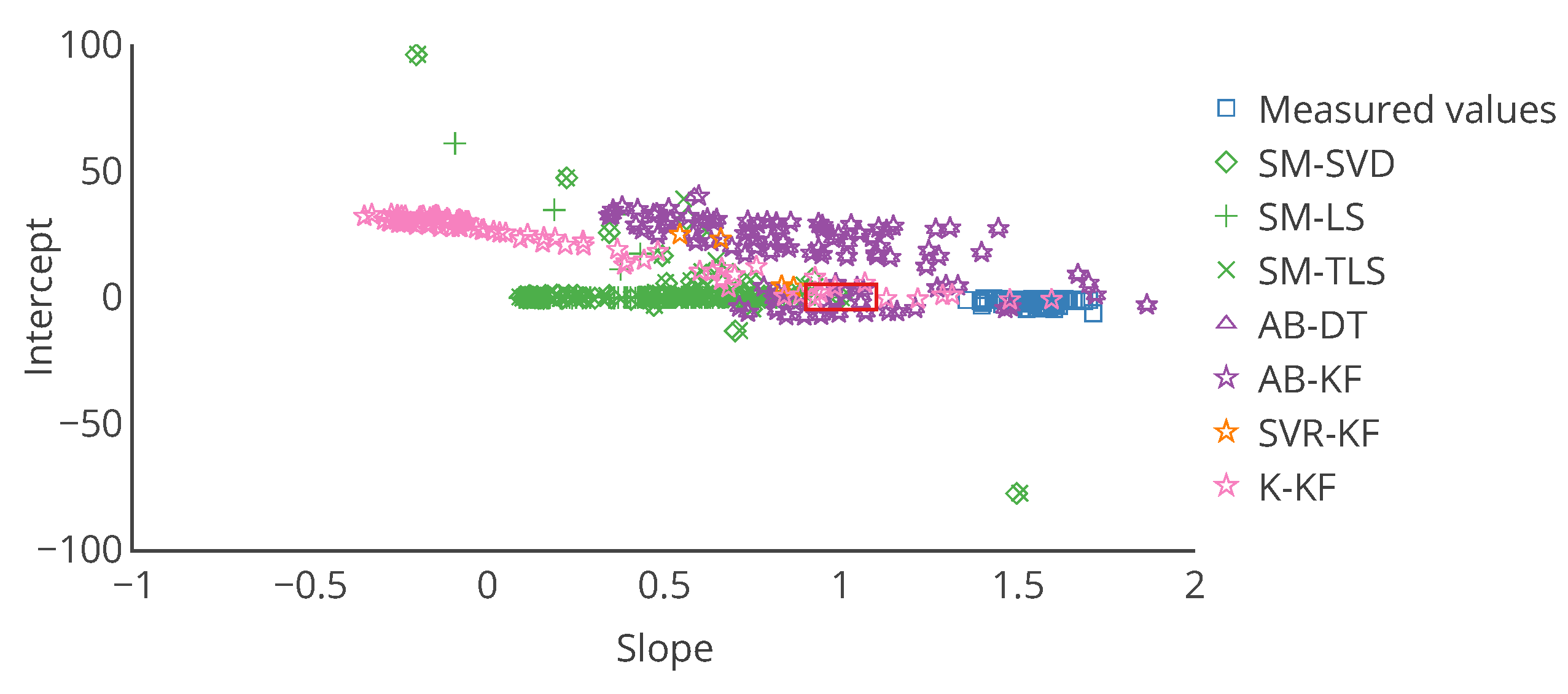
Figure 14.
Target plot of the 16 nodes as a function of their slope and intercept in the error model, computed on the entire time interval of drift, for each calibration strategy and with the Gaussian plume model. The instruments are not all present, notably for those after the correction by SVR-KF. Axis were truncated to keep the plot readable. The red rectangle depicts the same requirement as in
Figure 11 for example, a slope in
and an intercept in
. Few instruments are inside this area whatever the in situ calibration strategy considered.
Figure 15.
Evolution of the mean of the MAE, computed on the entire time interval of study, of all the nodes of the network, as a function of the number of nodes , for the 2D Gauss model.
Figure 15.
Evolution of the mean of the MAE, computed on the entire time interval of study, of all the nodes of the network, as a function of the number of nodes , for the 2D Gauss model.
Figure 16.
Target plot of the 16 nodes as a function of their slope and intercept in the error model, computed on the entire time interval of study, for each calibration strategy and with the Gaussian plume model. The instruments are not all present: axes were truncated to keep the plot readable. The red rectangle depicts the same requirement as in
Figure 11 and
Figure 14 for example, a slope in
and an intercept in
. More instruments are inside this area compared to
Figure 14 but most of them are outside whatever the in situ calibration strategy considered.
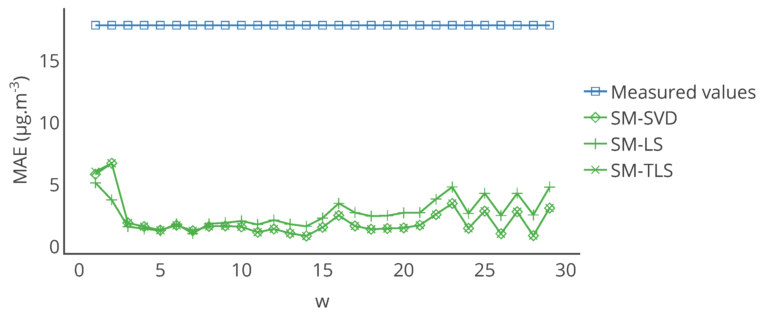
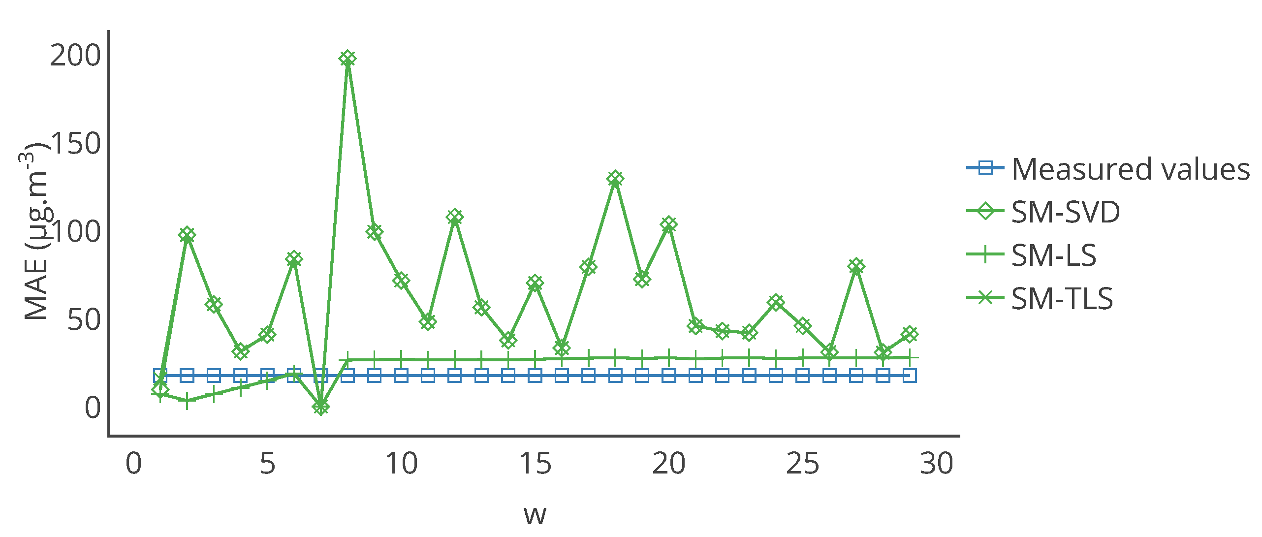
Figure 17.
Evolution of the mean of MAE, computed on the entire time interval of study, over the network for the strategies SM-SVD, SM-LS and SM-TLS as a function of
w. The best result is obtained for
, which was our original value in
Section 4, considering the average error of the three strategies for the same
w.
Figure 18.
Evolution of the mean of MAE, computed on the entire time interval of study, over the network for the strategies SM-SVD, SM-LS and SM-TLS as a function of
w with a different signal subspace than in
Figure 17. The best results are still obtained for
but for most the values of
w, the algorithms degrade the quality of the measurements and more significantly for SM-SVD and SM-TLS.
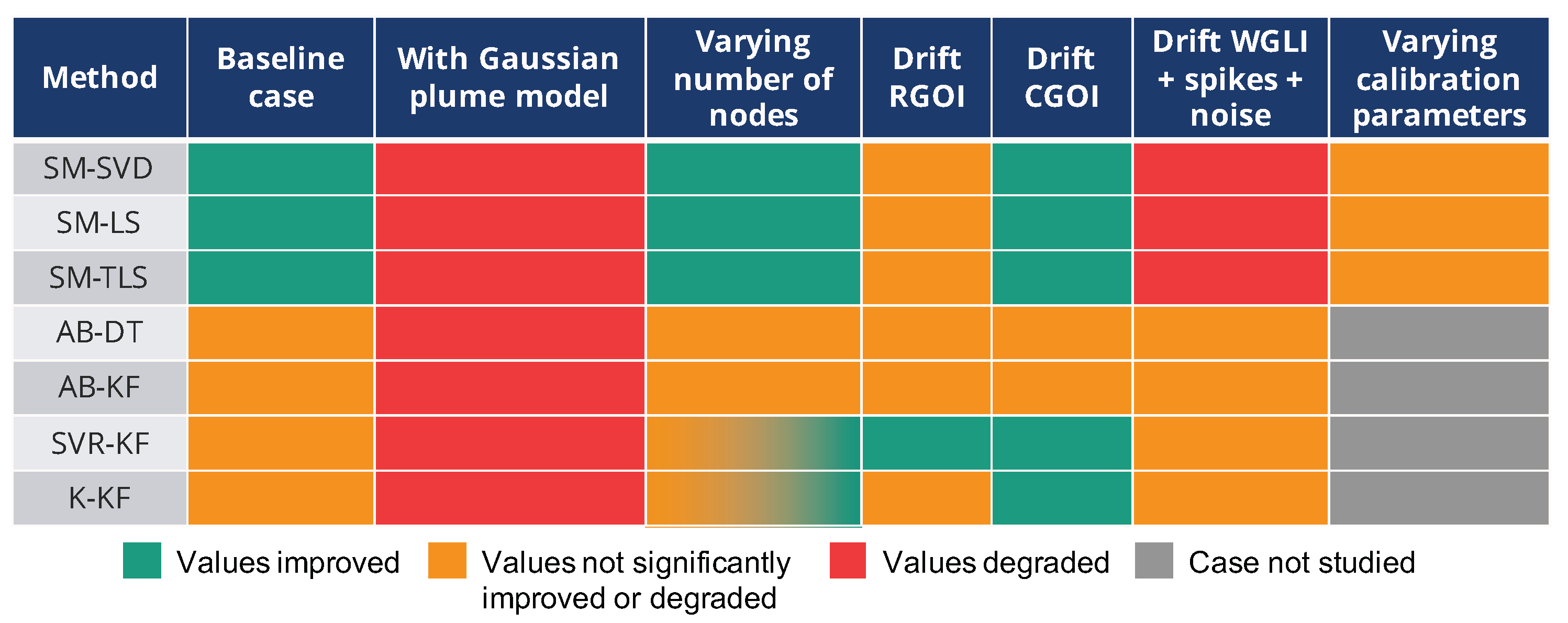
Figure 19.
Summary of the results observed by changing the parameters of the baseline case study which was built with a 2D Gaussian function to model the measurand, with the WGLI drift model applied to the measured values of the instruments, with 16 nodes in the network and the values indicated in
Section 4 for the parameters of the in situ calibration algorithms. The improvements are judged relatively to results of the baseline case, recalled in the first column. Thus, this table does not indicate that the corrected values are very close to the true values when the measured values are improved.
Table 1.
Mean and standard deviation of each metric, computed on the entire time interval of drift, over the 16 nodes of the network. SM-(SVD, LS, TLS) strategies have the best results overall whatever the metric considered. SVR-KF provides corrected values only slightly better than before calibration according to MAE and RMSE but not according to MAPE and Pearson correlation coefficient. AB-(DT, KF) and K-KF do not improve the measured values significantly.
| | MAE | | MAPE | | RMSE | | Pearson |
|---|
| | | | | | | | | | | | |
| No calibration | 18 | 2 | | 53 | 6 | | 25 | 2 | | 0.935 | 0.007 |
| SM-SVD | 1 | 1 | | 5 | 4 | | 2 | 2 | | 0.994 | 0.006 |
| SM-LS | 1 | 1 | | 3 | 2 | | 2 | 1 | | 0.995 | 0.005 |
| SM-TLS | 1 | 1 | | 5 | 4 | | 2 | 2 | | 0.994 | 0.006 |
| AB-DT | 18 | 1 | | 55 | 6 | | 25 | 1 | | 0.932 | 0.004 |
| AB-KF | 18 | 1 | | 58 | 11 | | 25 | 1 | | 0.933 | 0.003 |
| SVR-KF | 16 | 1 | | 83 | 11 | | 18 | 1 | | 0.825 | 0.012 |
| K-KF | 18 | 1 | | 53 | 10 | | 24 | 1 | | 0.927 | 0.005 |
Table 2.
Values of the metrics, computed on the entire time interval of drift, for two particular sensors of the network
and
. Strategies AB-(DT, KF) and (SVR, K)-KF are quite equivalent for these two instruments. The improvements are rather small for both sensors. For SM-(SVD, LS, TLS), results are consistent with the observations of
Table 1.
| | MAE | | MAPE | | RMSE | | Pearson |
|---|
| | | | | | | | | | | | |
| No calibration | 22 | 18 | | 66 | 51 | | 30 | 24 | | 0.924 | 0.942 |
| SM-SVD | 1 | 3 | | 4 | 10 | | 2 | 5 | | 0.996 | 0.983 |
| SM-LS | 1 | 2 | | 3 | 7 | | 2 | 3 | | 0.997 | 0.986 |
| SM-TLS | 1 | 3 | | 4 | 10 | | 2 | 5 | | 0.996 | 0.983 |
| AB-DT | 20 | 17 | | 61 | 49 | | 26 | 23 | | 0.933 | 0.932 |
| AB-KF | 18 | 17 | | 56 | 45 | | 25 | 23 | | 0.935 | 0.927 |
| SVR-KF | 16 | 16 | | 80 | 71 | | 19 | 19 | | 0.828 | 0.805 |
| K-KF | 17 | 16 | | 51 | 43 | | 24 | 23 | | 0.930 | 0.918 |
Table 3.
Mean and standard deviation of the weekly mean of each metric for
during the drift period. From the standard deviations of MAE, MAPE and RMSE, the observations made based on
Table 1 could be locally false, for example, a strategy is better than others considering a computation of the metrics over the 12 weeks of drift but not always considering a computation of the metrics over each week.
| | MAE | | MAPE | | RMSE | | Pearson |
|---|
| | | | | | | | | | | | |
| No calibration | 22 | 16 | | 66 | 36 | | 25 | 17 | | 1.000 | 0.000 |
| SM-SVD | 1 | 1 | | 3 | 3 | | 1 | 1 | | 1.000 | 0.000 |
| SM-LS | 1 | 1 | | 3 | 2 | | 1 | 1 | | 1.000 | 0.000 |
| SM-TLS | 1 | 1 | | 3 | 3 | | 1 | 1 | | 1.000 | 0.000 |
| AB-DT | 20 | 13 | | 61 | 32 | | 22 | 14 | | 0.999 | 0.001 |
| AB-KF | 18 | 13 | | 56 | 31 | | 21 | 14 | | 0.999 | 0.000 |
| SVR-KF | 16 | 4 | | 80 | 39 | | 18 | 4 | | 0.935 | 0.034 |
| K-KF | 17 | 14 | | 51 | 32 | | 20 | 15 | | 1.000 | 0.000 |
Table 4.
Mean (
) and standard deviation (
) of the parameters of the error model and the regression score, computed on the entire time interval of drift, over the 16 nodes of the network. The observations that can be made with these values are identical to those of
Table 1. This table also seems to confirm that there is a bias for SVR-KF as the standard deviation of the slope and intercept among sensors is small, with mean slope close to 1 but a mean intercept equal to 10. However, the poor mean score of the regression invites to be careful with this statement.
| | Slope | | Intercept | | Score |
|---|
| | | | | | | | | |
| No calibration | 1.62 | 0.07 | | −2 | 0 | | 0.87 | 0.01 |
| SM-SVD | 1.02 | 0.02 | | 1 | 0 | | 0.99 | 0.01 |
| SM-LS | 0.97 | 0.02 | | 1 | 0 | | 0.99 | 0.01 |
| SM-TLS | 1.02 | 0.02 | | 1 | 0 | | 0.99 | 0.01 |
| AB-DT | 1.62 | 0.05 | | −2 | 1 | | 0.87 | 0.01 |
| AB-KF | 1.62 | 0.04 | | −1 | 1 | | 0.87 | 0.01 |
| SVR-KF | 1.05 | 0.03 | | 10 | 1 | | 0.68 | 0.02 |
| K-KF | 1.62 | 0.04 | | −2 | 1 | | 0.86 | 0.01 |
Table 5.
Values of the parameters of the error model and the regression score, computed on the entire time interval of drift, for two particular sensors of the network
and
. The observations that can be made with these values are identical to those of
Table 2.
Table 5.
Values of the parameters of the error model and the regression score, computed on the entire time interval of drift, for two particular sensors of the network
and
. The observations that can be made with these values are identical to those of
Table 2.
| | Slope | | Intercept | | Score |
|---|
| | | | | | | | | |
| No calibration | 1.77 | 1.58 | | −2 | −1 | | 0.85 | 0.89 |
| SM-SVD | 1.01 | 1.05 | | 0 | 1 | | 0.99 | 0.97 |
| SM-LS | 0.97 | 0.94 | | 0 | 1 | | 0.99 | 0.97 |
| SM-TLS | 1.01 | 1.05 | | 0 | 1 | | 0.99 | 0.97 |
| AB-DT | 1.62 | 1.55 | | 0 | −1 | | 0.87 | 0.87 |
| AB-KF | 1.63 | 1.56 | | −1 | −3 | | 0.87 | 0.86 |
| SVR-KF | 1.09 | 1.01 | | 9 | 12 | | 0.69 | 0.65 |
| K-KF | 1.62 | 1.56 | | −2 | −4 | | 0.87 | 0.84 |
Table 6.
Mean (
) and standard deviation (
) of the parameters of the error model and the regression score for
, computed on each week of the drift period. The slope for SVR-KF varies significantly and the mean intercept is equal to zero with a standard deviation of 17. This is not the case for the other strategies. Thus, the observation made with
Table 5 on SVR-KF is not valid locally and can explain why the mean score is poor compared to the ones obtained with the other strategies.
| | Slope | | Intercept | | Score |
|---|
| | | | | | | | | |
| No calibration | 1.66 | 0.36 | | 0 | 0 | | 1.00 | 0.00 |
| SM-SVD | 1.03 | 0.04 | | 0 | 0 | | 1.00 | 0.00 |
| SM-LS | 0.99 | 0.03 | | 0 | 0 | | 1.00 | 0.00 |
| SM-TLS | 1.03 | 0.04 | | 0 | 0 | | 1.00 | 0.00 |
| AB-DT | 1.53 | 0.28 | | 2 | 1 | | 1.00 | 0.00 |
| AB-KF | 1.54 | 0.30 | | 0 | 1 | | 1.00 | 0.00 |
| SVR-KF | 1.35 | 0.28 | | 0 | 17 | | 0.88 | 0.06 |
| K-KF | 1.51 | 0.32 | | 0 | 0 | | 1.00 | 0.00 |
Table 7.
Mean and standard deviation of each metric, computed on the entire time interval of drift, over the 16 nodes of the network with the Gaussian plume model. No calibration strategy allows to obtain less error than without calibration, even for SM-(SVD, LS, TLS) strategies that had the best performances in
Section 4.
| | MAE | | MAPE | | RMSE | | Pearson | | Slope | | Intercept | | Score |
|---|
| | | | | | | | | | | | | | | | | | | | | |
| No calibration | 13 | 6 | | 17 | 6 | | 38 | 21 | | 0.98 | 0.00 | | 1.56 | 0.08 | | −2 | 1 | | 0.97 | 0.01 |
| SM-SVD | | | | | | | | | | 0.55 | 0.43 | | −21.11 | 60.40 | | | | | 0.48 | 0.42 |
| SM-LS | 26 | 24 | | 952 | | | 93 | 138 | | 0.85 | 0.34 | | 0.34 | 0.32 | | 10 | 28 | | 0.83 | 0.33 |
| SM-TLS | | | | | | | | | | 0.55 | 0.43 | | −21.11 | 60.40 | | | | | 0.48 | 0.42 |
| AB-DT | 36 | 3 | | | 529 | | 54 | 7 | | 0.62 | 0.19 | | 0.82 | 0.31 | | 19 | 13 | | 0.42 | 0.24 |
| AB-KF | 36 | 3 | | | 529 | | 54 | 7 | | 0.62 | 0.19 | | 0.82 | 0.31 | | 19 | 13 | | 0.42 | 0.24 |
| SVR-KF | 249 | 357 | | | | | 270 | 380 | | 0.54 | 0.18 | | 0.83 | 0.19 | | 234 | 357 | | 0.32 | 0.19 |
| K-KF | 47 | 22 | | | | | 85 | 36 | | 0.11 | 0.43 | | 0.26 | 0.66 | | 30 | 15 | | 0.18 | 0.27 |
Table 8.
Values of the metrics, computed on the entire time interval of drift, for two particular sensors of the network
and
, with the Gaussian plume model. No calibration strategy allows to obtain less error than without calibration, even for SM-(SVD, LS, TLS) strategies that had the best performances in
Section 4, despite apparently satisfying results according to MAE but not according to the slope and intercept notably.
| | MAE | | MAPE | | RMSE | | Pearson | | Slope | | Intercept | | Score |
|---|
| | | | | | | | | | | | | | | | | | | | | |
| No calibration | 12 | 12 | | 19 | 13 | | 36 | 35 | | 0.98 | 0.98 | | 1.75 | 1.47 | | −1 | −2 | | 0.96 | 0.97 |
| SM-SVD | 6 | 33 | | 108 | 201 | | 24 | 269 | | 0.83 | 0.06 | | 0.83 | 0.25 | | 2 | −6 | | 0.68 | 0.00 |
| SM-LS | 8 | 25 | | 55 | 86 | | 20 | 57 | | 0.97 | 0.97 | | 0.58 | 0.17 | | 0 | 0 | | 0.94 | 0.93 |
| SM-TLS | 6 | 33 | | 108 | 201 | | 24 | 269 | | 0.83 | 0.06 | | 0.83 | 0.25 | | 2 | −6 | | 0.68 | 0.00 |
| AB-DT | 37 | 32 | | | | | 51 | 45 | | 0.57 | 0.79 | | 0.77 | 0.92 | | 27 | 14 | | 0.33 | 0.63 |
| AB-KF | 37 | 32 | | | | | 51 | 45 | | 0.57 | 0.79 | | 0.77 | 0.92 | | 28 | 14 | | 0.33 | 0.63 |
| SVR-KF | 24 | 387 | | | | | 34 | 415 | | 0.69 | 0.34 | | 0.78 | 0.98 | | 3 | 382 | | 0.48 | 0.12 |
| K-KF | 27 | 63 | | 818 | | | 55 | 100 | | 0.60 | −0.25 | | 0.95 | -0.26 | | 18 | 42 | | 0.36 | 0.06 |
Table 9.
Mean and standard deviation of each metric, computed on the entire time interval of study, over the 100 nodes of the network with the Gaussian plume model. Again, no calibration strategy allows to obtain less error than without calibration.
Table 9.
Mean and standard deviation of each metric, computed on the entire time interval of study, over the 100 nodes of the network with the Gaussian plume model. Again, no calibration strategy allows to obtain less error than without calibration.
| | MAE | | MAPE | | RMSE | | Pearson | | Slope | | Intercept | | Score |
|---|
| | | | | | | | | | | | | | | | | | | | | |
| No calibration | 13 | 7 | | 17 | 6 | | 38 | 25 | | 0.98 | 0.00 | | 1.55 | 0.07 | | -2 | 1 | | 0.97 | 0.01 |
| SM-SVD | | | | | | | | | | 0.55 | 0.37 | | | | | | | | 0.43 | 0.38 |
| SM-LS | | | | | | | | | | 0.91 | 0.26 | | | | | | | | 0.89 | 0.26 |
| SM-TLS | | | | | | | | | | 0.54 | 0.37 | | | | | | | | 0.42 | 0.38 |
| AB-DT | 37 | 3 | | | 580 | | 57 | 8 | | 0.63 | 0.20 | | 1.02 | 0.71 | | 17 | 14 | | 0.43 | 0.25 |
| AB-KF | 37 | 3 | | | 578 | | 57 | 8 | | 0.63 | 0.20 | | 1.02 | 0.71 | | 17 | 14 | | 0.43 | 0.25 |
| SVR-KF | 412 | 208 | | | | | 432 | 232 | | 0.51 | 0.18 | | 0.82 | 0.14 | | 415 | 208 | | 0.29 | 0.16 |
| K-KF | 39 | 21 | | | 973 | | 71 | 41 | | 0.10 | 0.44 | | 0.19 | 1.38 | | 23 | 11 | | 0.20 | 0.30 |
Table 10.
Values of the metrics, computed on the entire time interval of study, for two particular sensors of the network
and
, with the Gaussian plume model. For these instruments, the results are quite equivalent to those of
Table 8 in orders of magnitude.
Table 10.
Values of the metrics, computed on the entire time interval of study, for two particular sensors of the network
and
, with the Gaussian plume model. For these instruments, the results are quite equivalent to those of
Table 8 in orders of magnitude.
| | MAE | | MAPE | | RMSE | | Pearson | | Slope | | Intercept | | Score |
|---|
| | | | | | | | | | | | | | | | | | | | | |
| No calibration | 10 | 10 | | 22 | 22 | | 23 | 21 | | 0.98 | 0.99 | | 1.59 | 1.54 | | −1 | −1 | | 0.97 | 0.97 |
| SM-SVD | 5 | 3 | | 36 | 25 | | 13 | 6 | | 0.92 | 0.99 | | 0.84 | 0.87 | | 0 | 0 | | 0.85 | 0.98 |
| SM-LS | 6 | 4 | | 42 | 30 | | 11 | 6 | | 0.99 | 1.00 | | 0.71 | 0.84 | | 0 | 0 | | 0.99 | 0.99 |
| SM-TLS | 5 | 3 | | 36 | 25 | | 13 | 6 | | 0.92 | 0.99 | | 0.84 | 0.87 | | 0 | 0 | | 0.85 | 0.98 |
| AB-DT | 37 | 37 | | | | | 53 | 54 | | 0.59 | 0.63 | | 1.11 | 1.28 | | 20 | 16 | | 0.35 | 0.39 |
| AB-KF | 38 | 37 | | | | | 53 | 54 | | 0.59 | 0.63 | | 1.11 | 1.28 | | 20 | 16 | | 0.34 | 0.39 |
| SVR-KF | 373 | 309 | | | | | 374 | 311 | | 0.63 | 0.68 | | 0.89 | 1.02 | | 375 | 309 | | 0.39 | 0.46 |
| K-KF | 9 | 10 | | 44 | 62 | | 18 | 22 | | 0.95 | 0.90 | | 1.31 | 1.29 | | 1 | 1 | | 0.91 | 0.81 |
Table 11.
Mean and standard deviation of each metric, computed on the entire time interval of study, over the 16 nodes of the network with the RGOI drift model. Results are very different with this model compared to
Table 1 and
Table 4, notably for SM-(SVD, LS, TLS) even if we take into account that we expected to have incorrect offsets.
| | MAE | | MAPE | | RMSE | | Pearson | | Slope | | Intercept | | Score |
|---|
| | | | | | | | | | | | | | | | | | | | | |
| No calibration | 56 | 0 | | 273 | 46 | | 65 | 0 | | 0.65 | 0.00 | | 1.41 | 0.00 | | 43 | 1 | | 0.42 | 0.01 |
| SM-SVD | 50 | 3 | | 248 | 32 | | 56 | 3 | | 0.67 | 0.01 | | 1.24 | 0.01 | | 42 | 2 | | 0.45 | 0.01 |
| SM-LS | 46 | 1 | | 232 | 43 | | 52 | 1 | | 0.68 | 0.00 | | 1.18 | 0.04 | | 40 | 0 | | 0.46 | 0.00 |
| SM-TLS | 50 | 3 | | 248 | 32 | | 56 | 3 | | 0.67 | 0.01 | | 1.24 | 0.01 | | 42 | 2 | | 0.45 | 0.01 |
| AB-DT | 56 | 0 | | 274 | 48 | | 65 | 0 | | 0.65 | 0.00 | | 1.41 | 0.01 | | 43 | 1 | | 0.42 | 0.00 |
| AB-KF | 56 | 1 | | 276 | 54 | | 65 | 1 | | 0.64 | 0.00 | | 1.41 | 0.03 | | 43 | 1 | | 0.42 | 0.00 |
| SVR-KF | 14 | 0 | | 86 | 13 | | 16 | 1 | | 0.84 | 0.01 | | 0.76 | 0.02 | | 20 | 1 | | 0.71 | 0.02 |
| K-KF | 56 | 1 | | 276 | 54 | | 65 | 1 | | 0.64 | 0.00 | | 1.41 | 0.03 | | 43 | 1 | | 0.41 | 0.00 |
Table 12.
Mean and standard deviation of each metric, computed on the entire time interval of study, over the 16 nodes of the network with the CGOI drift model. Results are very different with this model compared to
Table 1 and
Table 4, notably for SM-(SVD, LS, TLS) even if we take into account that we expected to have incorrect offsets.
| | MAE | | MAPE | | RMSE | | Pearson | | Slope | | Intercept | | Score |
|---|
| | | | | | | | | | | | | | | | | | | | | |
| No calibration | 44 | 29 | | 210 | 131 | | 51 | 34 | | 0.75 | 0.15 | | 1.34 | 0.20 | | 33 | 23 | | 0.58 | 0.23 |
| SM-SVD | 33 | 21 | | 162 | 99 | | 38 | 24 | | 0.78 | 0.14 | | 1.18 | 0.12 | | 27 | 17 | | 0.63 | 0.21 |
| SM-LS | 26 | 16 | | 133 | 89 | | 31 | 19 | | 0.77 | 0.13 | | 1.07 | 0.13 | | 21 | 14 | | 0.61 | 0.20 |
| SM-TLS | 33 | 21 | | 162 | 99 | | 38 | 24 | | 0.78 | 0.14 | | 1.18 | 0.12 | | 27 | 17 | | 0.63 | 0.21 |
| AB-DT | 46 | 1 | | 227 | 44 | | 54 | 1 | | 0.70 | 0.01 | | 1.35 | 0.03 | | 35 | 1 | | 0.49 | 0.01 |
| AB-KF | 47 | 1 | | 228 | 46 | | 54 | 1 | | 0.70 | 0.00 | | 1.35 | 0.03 | | 36 | 1 | | 0.49 | 0.00 |
| SVR-KF | 14 | 0 | | 85 | 13 | | 16 | 0 | | 0.84 | 0.01 | | 0.76 | 0.02 | | 20 | 1 | | 0.71 | 0.02 |
| K-KF | 20 | 1 | | 95 | 22 | | 23 | 1 | | 0.89 | 0.00 | | 1.18 | 0.02 | | 14 | 1 | | 0.79 | 0.01 |
Table 13.
Mean and standard deviation of each metric, computed on the entire time interval of study, over the 16 nodes of the network with the WGLI drift model, spikes and noise. The results with SM-(SVD, LS, TLS) are significantly influenced by the spikes and noise. The other strategies do not seem to provide more degraded results due to the noise and spikes although the performances were fairly unsatisfying from the start in
Section 4.
| | MAE | | MAPE | | RMSE | | Pearson | | Slope | | Intercept | | Score |
|---|
| | | | | | | | | | | | | | | | | | | | | |
| No calibration | 25 | 2 | | 106 | 14 | | 33 | 2 | | 0.79 | 0.01 | | 1.62 | 0.07 | | –2 | 0 | | 0.62 | 0.01 |
| SM-SVD | 60 | 50 | | 198 | 144 | | 82 | 70 | | 0.23 | 0.33 | | 0.18 | 0.69 | | –13 | 14 | | 0.16 | 0.25 |
| SM-LS | 28 | 6 | | 93 | 10 | | 33 | 7 | | 0.35 | 0.57 | | 0.15 | 0.26 | | 0 | 1 | | 0.43 | 0.08 |
| SM-TLS | 60 | 50 | | 198 | 144 | | 82 | 70 | | 0.23 | 0.33 | | 0.18 | 0.69 | | –13 | 14 | | 0.16 | 0.25 |
| AB-DT | 21 | 1 | | 78 | 17 | | 28 | 2 | | 0.88 | 0.01 | | 1.63 | 0.04 | | –2 | 1 | | 0.77 | 0.02 |
| AB-KF | 21 | 1 | | 78 | 17 | | 28 | 2 | | 0.88 | 0.01 | | 1.63 | 0.04 | | –1 | 1 | | 0.78 | 0.02 |
| SVR-KF | 18 | 0 | | 92 | 15 | | 22 | 0 | | 0.75 | 0.01 | | 1.06 | 0.03 | | 10 | 1 | | 0.56 | 0.01 |
| K-KF | 25 | 1 | | 107 | 18 | | 32 | 1 | | 0.79 | 0.00 | | 1.61 | 0.04 | | –2 | 1 | | 0.62 | 0.01 |


