Monitoring the Effects of Water Stress in Cotton Using the Green Red Vegetation Index and Red Edge Ratio


1
Centre for Regional and Rural Futures (CeRRF), Deakin University, Griffith, NSW 2680, Australia
2
School of Science and Technology, University of New England, Armidale, NSW 2350, Australia
*
Author to whom correspondence should be addressed.
Remote Sens. 2019, 11(7), 873; https://doi.org/10.3390/rs11070873
Submission received: 28 February 2019
/
Revised: 26 March 2019
/
Accepted: 8 April 2019
/
Published: 10 April 2019
(This article belongs to the Special Issue Remote Sensing for Crop Water Management)
Abstract
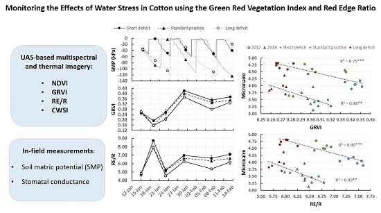
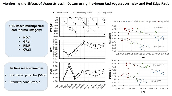
:The main objective of this work was to study the feasibility of using the green red vegetation index (GRVI) and the red edge ratio (RE/R) obtained from UAS imagery for monitoring the effects of soil water deficit and for predicting fibre quality in a surface-irrigated cotton crop. The performance of these indices to track the effects of water stress on cotton was compared to that of the normalised difference vegetation index (NDVI) and crop water stress index (CWSI). The study was conducted during two consecutive seasons on a commercial farm where three irrigation frequencies and two nitrogen rates were being tested. High-resolution multispectral images of the site were acquired on four dates in 2017 and six dates in 2018, encompassing a range of matric potential values. Leaf stomatal conductance was also measured at the image acquisition times. At harvest, lint yield and fibre quality (micronaire) were determined for each treatment. Results showed that within each year, the N rates tested (> 180 kg N ha−1) did not have a statistically significant effect on the spectral indices. Larger intervals between irrigations in the less frequently irrigated treatments led to an increase (p < 0.05) in the CWSI and a reduction (p < 0.05) in the GRVI, RE/R, and to a lesser extent in the NDVI. A statistically significant and good correlation was observed between the GRVI and RE/R with soil matric potential and stomatal conductance at specific dates. The GRVI and RE/R were in accordance with the soil and plant water status when plants experienced a mild level of water stress. In most of the cases, the GRVI and RE/R displayed long-term effects of the water stress on plants, thus hampering their use for determinations of the actual soil and plant water status. The NDVI was a better predictor of lint yield than the GRVI and RE/R. However, both GRVI and RE/R correlated well (p < 0.01) with micronaire in both years of study and were better predictors of micronaire than the NDVI. This research presents the GRVI and RE/R as good predictors of fibre quality with potential to be used from satellite platforms. This would provide cotton producers the possibility of designing specific harvesting plans in the case that large fibre quality variability was expected to avoid discount prices. Further research is needed to evaluate the capability of these indices obtained from satellite platforms and to study whether these results obtained for cotton can be extrapolated to other crops.
1. Introduction
Soil and plant water status monitoring is considered essential to properly manage irrigation of crops [1]. This is because maintaining an adequate soil water content and plant water status for each crop phenological stage is fundamental for good crop performance. Soil water deficit usually triggers a variety of physiological responses in plants, which if prolonged over time, may detrimentally affect plant growth and yield [2]. In the case of cotton (Gossypium hirsutum L.), water stress has been linked to a decrease in stomatal conductance and photosynthesis [3], reduction of leaf water potential and the Rubisco binding protein content as well as an increase in anthocyanin content [4]. Water stress may reduce plant growth and total number of bolls at harvest due to a decrease in the total fruiting positions as well as boll shedding, which detrimentally affects lint yield [5]. Cotton is more sensitive to water stress at early stages of the crop than later in the season although severe water stress from peak bloom to maturity may also have a negative impact on lint yield and fibre quality [6]. Lint quality parameters such as fibre length and micronaire, for instance, can be impaired when the crop is water stressed from early to mid-boll filling stage [7]. Severe water stress during this period may significantly increase micronaire, which can prevent cotton producers from meeting the quality standards needed to achieve premium prices.
Detection of some of the physiological changes in plants in response to water stress is the basis of conventional and alternative plant-based methods for crop water status monitoring (see [8,9]). Methods such as the measurement of the stomatal conductance, leaf water potential and sap flow, among others, have been successfully used in cotton to detect plant water stress [10,11,12]. These methods, however, are based on data collected from a few point source locations of a field, which may not be representative of the current crop water status at the field scale. Sensing of crops from platforms such as satellites or unmanned aerial systems (UASs) allows large areas to be monitored and thus presents as a more appropriate method to use for extensively planted crops such as cotton. The flexibility in terms of revisit of the sites, improvement in flight times and the higher resolution that the use of low-cost UASs present in comparison to traditional satellites make the UASs an interesting platform to use for crop monitoring.
Studies have shown that UAS-based thermal images can be used to estimate leaf water potential and map within-field crop water status variability in cotton [13]. This is possible because soil water deficit often leads plants to close their stomata, decreasing canopy stomatal conductance and transpiration, which in turn raises canopy temperature (Tc) [14]. Thus, water-stressed plants will exhibit higher Tc values than non-stressed plants. Expressing the Tc values of a crop relative to a minimum and maximum levels of stress (wet and dry baselines, respectively), which can be obtained by either empirical or theoretical methods [15,16], is the basis of the so-called crop water stress index (CWSI). The authors of [13] calculated the CWSI using Tc obtained from pure vegetation pixels based on [17], air temperature (Ta) plus 5 °C as the dry baseline and compared the results using several alternatives for the wet reference (representative of a fully transpiring leaves), aiming to map cotton water status at a commercial scale. Among the alternatives explored, the best results were obtained using a theoretical (energy balance equation) or bio-indicator references, such as the average temperature of the coolest 5–10% canopy pixels or the temperature of a wet leaf. High-resolution thermal imagery obtained from UASs has been successfully used also in grapevines and fruit trees to scale up water potential measurements from a single leaf to the farm level [18,19,20].
Unlike Tc, indices that can track non-stomatal reductions of photosynthesis under soil water deficit, such as changes in photosynthetic pigments, are also of great interest because they can provide relevant insight into the physiological performance of crops ([9] and references therein). Pigments are the dominant factor determining leaf reflectance in the visible wavelength (400–700 nm), with chlorophyll considered the most relevant pigment for water stress detection [21]. Changes in foliage colour from bluish green to dark green have been long pointed out as a visual indicator of the onset of water stress in cotton and other crops such as beans and peanuts [22]. Under sustained soil water deficit, leaf chlorophyll content often decreases, leading to a reduction in green reflection and an increase in blue and red reflections [23]. The transition region of the reflectance between the red and near infrared regions, named the red edge, has been proven to be sensitive to changes in leaf chlorophyll content [24]. Pigment-related indices including reflectance from the red edge band obtained from ground, UASs and satellite platforms have been well correlated with canopy chlorophyll content and total nitrogen content (directly related to chlorophyll content) in different crops [25,26,27]. The red edge ratio (RE/R) in particular, which includes information from the red edge and red bands, was shown as a good indicator of the chlorophyll content in a study conducted in a farm composed of five fruit tree crop species [28]. Other than chlorophyll, changes in carotenoid (e.g., xanthophyll pigments) and anthocyanin pigments have been also related to plant stresses including water stress [29,30].
Leaf moisture content as well as other aspects of crops such as leaf structure (e.g., cuticle thickness, number of air water interfaces, leaf hair, surface wax, etc.), leaf angle distribution and percentage of canopy cover, among others, may affect the relationship between spectral reflectance and pigment concentrations at both leaf and canopy scales [29,31]. Further, soil background effects can also detrimentally affect the correlation between vegetation indices (VIs) and remotely monitored biophysical variables [32], thus highlighting the importance of using vegetation-associated pixels for computing the VIs when possible. Research aimed at finding the best VIs to predict biophysical, biochemical and structural parameters of plants has shown that normalised difference spectral indices in which only two bands are used generally perform better than other type of indices [33,34]. That is the case of the green red vegetation index (GRVI), which includes information from the green and red bands and has been shown to correlate well with leaf water content [35]. The GRVI has been reported to detect changes in canopy vegetation and phenological stages, performing better in this task than the normalised difference vegetation index (NDVI) [36,37]. In [36], measurements were taken using a hemi-spherical spectro-radiometer and an automatic-capturing digital fish-eye camera installed on a mast at sites representative of four ecosystems in Japan. In [37], measurements from an UAS were performed to assess the feasibility of using the GRVI for determining the vegetation cover. Results showed the possibility of using the GRVI for crop cover and actual in-field evapotranspiration determinations of peanuts. The same study [37], also suggested from two flight campaigns conducted in a single season on a cotton field that irrigation water uniformity could be assessed by GRVI measurements.
The main objective of this work was to study the feasibility of using the pigment-related indices green red vegetation index (GRVI) and red edge ratio (RE/R) obtained from an UAS for monitoring the soil and plant water status in cotton as well as for predicting fibre quality. Cotton (Gossypium hirsutum L.) is a crop grown in almost eighty countries around the world (between the 45°N and 35°S parallels) because of its relevance for oilseed and fibre production. In Australia, where this study was conducted, cotton is a major commodity mainly grown in New South Wales (66% of the total production) and Queensland (33% of the total production) [38]. As an important product for the textile industry, cotton price is determined based on the quality of each cotton bale and thus, large variability in fibre quality is undesirable in a cotton field. Among the lint quality parameters, micronaire has been suggested as the best parameter for prediction in the field [39] and it is the parameter that was considered in this study. Micronaire variation has been shown to correlate in some extent with the variation in soil properties. Clay content and electrical conductivity among others, are soil-related factors that have been closely related to micronaire [39,40]. All these factors influence the soil water holding capacity and availability of water for the crop and thus, VIs that could track the effects of water stress on cotton could potentially be good predictors of fibre-quality.
The GRVI was selected because of its reported sensitivity to changes in canopy structure and green colour, both symptoms of water stress in cotton. Its higher performance as a phenology indicator than NDVI at full canopy cover points out the GRVI as a possible water stress indicator. The RE/R was tested because of its sensitivity to the chlorophyll content, which is reduced under sustained soil water deficit [28]. Further, both indices, GRVI and RE/R, have more potential for scaling to satellite data than thermal-based indices, which makes them more beneficial in practical use applications by farmers. Performance of these indices to monitor soil and plant water status of cotton was compared to that of the NDVI and CWSI, which have been extensively reported in the literature for water stress detection [9,41,42,43]. The specific objectives of the study were to (i) explore the relationships between the GRVI, RE/R, NDVI and CWSI with soil matric potential and stomatal conductance, which are indicators of the soil and plant water status, respectively; (ii) compare the performance of these indices in tracking the effects of water stress, and; (iii) assess their performance in predicting the effects of water stress on lint yield and fibre quality.
2. Materials and Methods
2.1. Location, Site Characteristics and Treatments
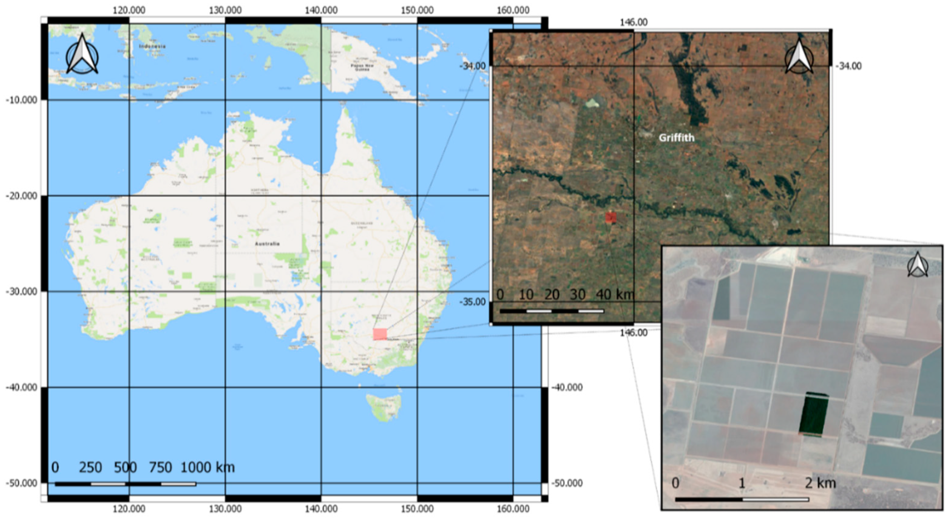
The study was performed during the 2016/17 and 2017/18 cotton-growing seasons in a commercial syphon-irrigated cotton farm located in the Murrumbidgee Valley at Darlington Point, NSW, Australia (Figure 1), where an irrigation x nitrogen interaction study was being conducted. The soil at the site was classified as Chromosol [44] with a 20 cm sandy clay loam A horizon over a dense clay B horizon. The climate in this area is semi-arid characterized by hot and dry summers, and cool winters.
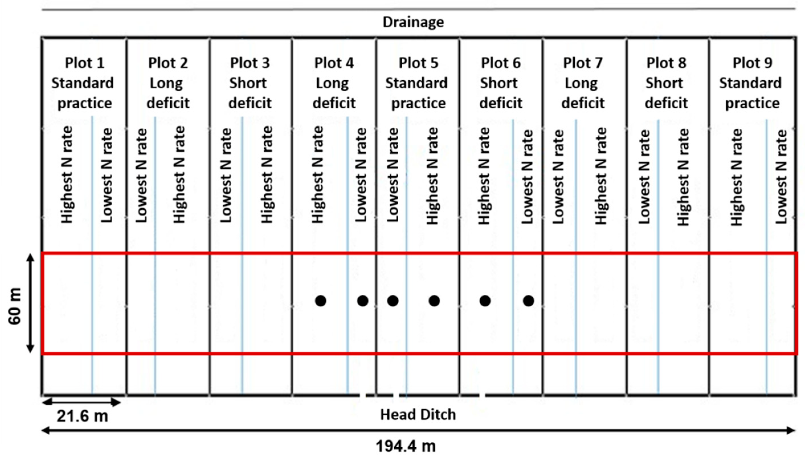
The cotton was sown on 17 October 2016 and 03 October 2017 with the variety SICOT 746BRF in beds of 1.80 m width at a row spacing of 0.90 m. The 1.16-ha area monitored in this study consisted of three irrigation and two nitrogen rate treatments distributed in a split plot design with irrigation as the main-plot factor replicated three times (nine main plots in total) and N rates as subplots. The dimension of the plots was 60.0 m × 21.6 m as illustrated in Figure 2. Thus, main plots had an area of 0.13 ha and consisted of 24 rows (12 beds), of which 16 rows received the highest N rate tested each year (277 and 309 kg N ha−1 the first and second season, respectively) and the remaining eight rows the lowest (180 kg N ha−1 in the 2016/17 season and 244 kg N ha−1 in the 2017/18). This was part of a larger study plot of 12.44 ha as illustrated in Figure 2. During the first season of study, fertiliser was applied as urea, broadcasted on 21 November 2016 and side dressed on 28 December 2016. In the 2017/18 cotton-growing season, fertiliser was applied as anhydrous ammonia (NH3-N) (at pre-planting) on 12 July 2017 and as side-dressed urea on 4 January 2018.
The irrigation strategies tested were a short deficit treatment, which was irrigated every seven days; a long deficit treatment irrigated at ≤ −100 kPa and; the standard irrigation practice in the area, which consists of watering approximately every two weeks. Irrigation treatments were imposed from around first flowering in early January to mid-February. The dates when irrigation was applied to each treatment within each growing season during the period of measurements are shown in Table 1.
An onsite weather station adjacent to the site recorded the meteorological conditions during the study.
2.2. In-Field Measurements
Soil matric potential was monitored continuously by means of watermark sensors (Model 200SS, Irrometer Company inc., California, USA) installed at the beginning of each growing season in pairs within the plant row at 0.23 m depth. Sensors were installed at the centre of two subplots (both N rates tested each year) of one main plot per irrigation treatment, giving a total of six stations (see Figure 2). Each station had two matric potential sensors attached to allow averaging of their readings to reduce uncertainty. All the soil moisture sensors (and the on-site weather station) were wired to WiField loggers (Goanna telemetry, Goondiwindi QLD, Australia), which periodically connected to the available WiFi network at the site to send data to a cloud-based data storage, processing and internet interface in real time [45]. Thus, soil matric potential readings for the long deficit treatment were used to advise the agronomist of the site when the imposed threshold value (−100 kPa) had been reached in order to trigger an irrigation event.
Leaf stomatal conductance measurements were performed with a leaf porometer (SC-1 Porometer, Decagon, WA, USA) in all the plots equipped with watermark sensors (six subplots in total), around noon and on the same dates when images of the site were acquired from the UAS. Measurements were taken on the fifth leaf below the terminal of six to eight plants per subplot (12–16 plants per irrigation treatment) distributed along the 60-m row where the watermark sensors were located.
2.3. Multispectral and Thermal Imagery
Multispectral images were acquired within two hours of solar noon during four dates in 2017 and six dates in 2018 from mid-January to mid-February (approximately from first flower to cut out). Images were taken with a 5-band multispectral camera (RedEdge, MicaSense Inc., Seattle, WA, USA) installed on an UAS (Inspire 1, DJI). Meteorological conditions [air temperature (Ta), relative humidity, solar radiation, wind speed and vapour pressure deficit] at the time when images were acquired are shown in Table 2. During the 2017/18 growing season, apart from the multispectral images, thermal images were also taken from the UAS with a thermal camera (Tau 2 640, FLIR Systems, Wilsonville, OR, USA).
Flight planning and automation was achieved using Drone Deploy on an iPad (http://www.dronedeploy.com/). This generated a flight path covering the field, ensuring sufficient overlap between subsequent image captures. The multispectral camera captured images corresponding to the spectral reflectance in the blue, green, red, red-edge and NIR bands centred at 475, 560, 668, 717 and 840 nm, respectively. The filter bandwidths were 20, 20, 10, 10 and 40 nm, respectively. The thermal camera has a resolution of 640 × 512 pixels and was configured to take images every second. The flight altitude for the multispectral and thermal images was set at 100 m and 60 m AGL (above ground level), respectively, which provided images with a ground resolution of 6.8 cm and 7.7 cm per pixel. The multispectral camera was configured to ensure 80% overlap between consecutive images, in order to ensure that an accurate orthomosaic could be generated. An image of a reflectance calibration panel was taken before and after each flight to remove effects of sunlight variation and reflectance characteristics. The set of multispectral images taken during each date was then processed using Pix4D where the individual image captures were stitched together using an orthomosaic process and where the reflectance was calibrated. For the thermal images, the TMC files from the thermal camera were first merged together using the ThermoViewer software and then exported in TIFF format with EXIF data for processing in Pix4D. The output was a single high-resolution GeoTIFF image of the whole site. The GeoTIFF thermal and multispectral images of each measurement date were then post-processed in QGIS (version 3.0.3) where vector grids with meshes of 10.8 m × 60 m and 3.6 m × 60 m were created for the subplots fertilised with the respective highest and lowest N rates each season leaving a two-row buffer between subplots. The NDVI, GRVI and RE/R indices were then computed from the multispectral images for each measurement date (see formulations at Table 3). Soil was filtered according to [37], where GRVI values below 0 within each measurement date were used to create a soil mask and filter most of the soil background. The zonal statistics tool available in QGIS was used to obtain the average and standard deviation data for each VI at each subplot.
The CWSI formulation is also shown in Table 3. CWSI was obtained according to [13]. Tc was obtained by first, separating canopy-related (Tcr) pixels from those of soil by using the thresholds (Ta − 10) < Tcr < (Ta + 7) and then taking the average temperature of the coldest 40% canopy-related pixels (thresholds recommended are between 25–50% according to [46]). The wet reference (Twet) was set as the average temperature of the 5% coldest pixels in the image. The dry reference (Tdry) was obtained by adding 5°C to the mean Ta for the period of measurements of each specific date.
2.4. Yield and Lint Quality
Lint yield was determined by weighing commercially picked field modules on a customized weigh trailer and multiplying using a 43% turn out factor. The seed lint was sub-sampled and quality determination, including micronaire, was conducted using a Uster High Volume Instrumentation 1000 at a commercial classing facility (ProClass Pty Ltd., Griffith NSW).
2.5. Statistical Analysis
Mean values of stomatal conductance, NDVI, GRVI, RE/R and CWSI for each treatment were compared using the SPSS v. 24.0 software (IBM Corp., Armonk, NY, USA) by means of a multiple comparison analysis using the Tukey’s Honest Significant Difference test at a significance level of 0.05. The relationship between the spectral indices and CWSI with stomatal conductance, soil matric potential, lint yield and fibre quality was explored by linear regression analyses with the statistical software Statgraphics Centurion XVI.
3. Results
3.1. Time Series of In-Field and Remote Sensing Measurements During the 2016/17 Growing Season
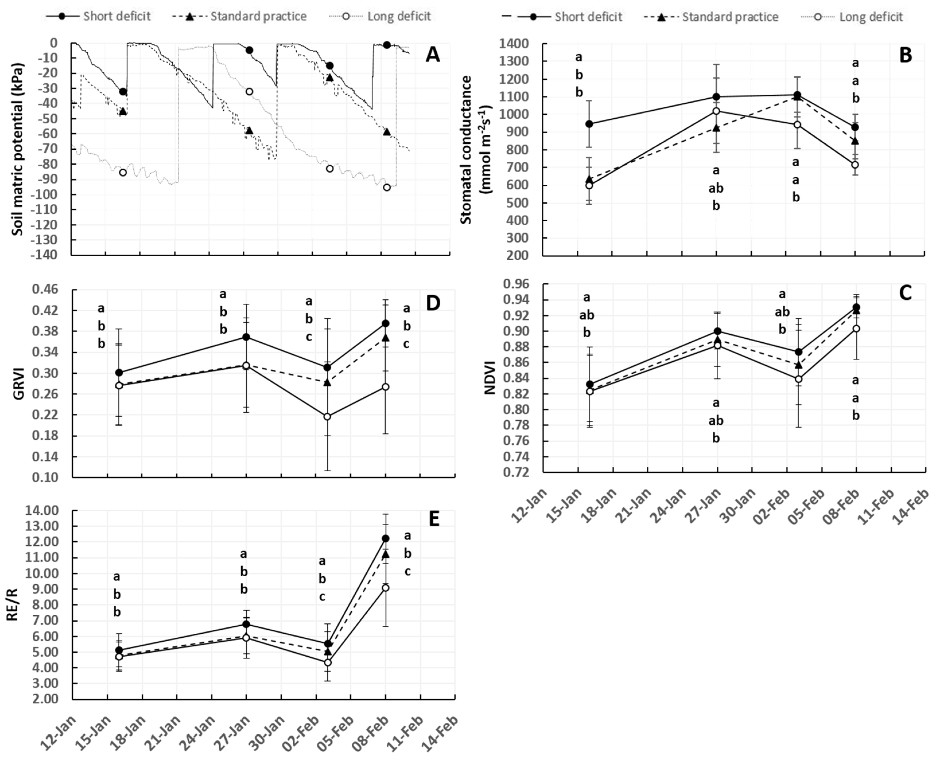
Mean values of soil matric potential, stomatal conductance, GRVI, NDVI and RE/R for each irrigation treatment during the period of measurements in 2016/17 are illustrated in Figure 3. No differences in stomatal conductance, NDVI, GRVI and RE/R were observed between N rate treatments (data not shown).
3.1.1. Soil and Plant Water Status
Watermark readings during the period of measurements showed that soil matric potential decreased in all the treatments between irrigation events (Figure 3A). Lower soil matric potential values were reached in the less frequently irrigated treatments (standard and long deficit) than in the short deficit treatment. Minimum readings of −42.1 kPa were reached in the short deficit treatment while minimum readings of −78.0 kPa and −95.0 kPa were reached in the standard practice and long deficit treatment, respectively. In all treatments, matric potential returned to values above −10 kPa after an irrigation event indicating that enough water was applied to replenish the soil profile. Mean soil matric potential at the time of the stomatal conductance and remote sensing measurements is also indicated in Figure 3A. The short deficit treatment had the highest soil matric potential (wettest soil) on all measurement dates. The long deficit treatment, on the other hand, had the lowest readings on all measurement dates with the exception of 27 January 2017, when the standard practice had not been irrigated for 10 days (four more than the long deficit) and thus, it had the lowest soil matric potential values.
The stomatal conductance measurements were in agreement with the soil matric potential readings (Figure 3B). The short deficit treatment had the highest stomatal conductance on all measurement dates. Values in this treatment ranged from 861 to 1174 mmol m−2 s−1. Less frequency of irrigation in the long deficit treatment led to a reduction (p < 0.05) in stomatal conductance in this treatment relative to the short deficit on all dates with the exception of 27 January 2017. In the standard practice, lower (p < 0.05) stomatal conductance values than in the short deficit were also observed the first two measurement dates on 16 and 27 January 2017.
3.1.2. Multispectral Indices
Mean values of NDVI, GRVI and RE/R followed a similar trend during the 2016/17 growing season (Figure 3C–E). The most frequently irrigated treatment (short deficit) had the highest values of NDVI, GRVI and RE/R during the whole season. During the period of measurements, mean values of these indices in the short deficit treatment ranged from 0.83 to 0.93 for the NDVI (Figure 3C), from 0.30 to 0.40 for the GRVI and from 5.0 to 12.0 for the RE/R. A statistically significant reduction (p < 0.05) in NDVI, GRVI and RE/R was observed in the long deficit treatment with respect to the short deficit on all dates. Compared to the short and long deficit treatments, the standard practice showed intermediate values of NDVI, GRVI and RE/R. The GRVI and RE/R values in the standard practice were lower (p < 0.05) than in the short deficit treatment on all dates. Differences in NDVI between the standard practice and the short deficit treatment were not statistically significant.
3.2. Time Series of In-Field and Remote Sensing Measurements During the 2017/2018 Growing Season
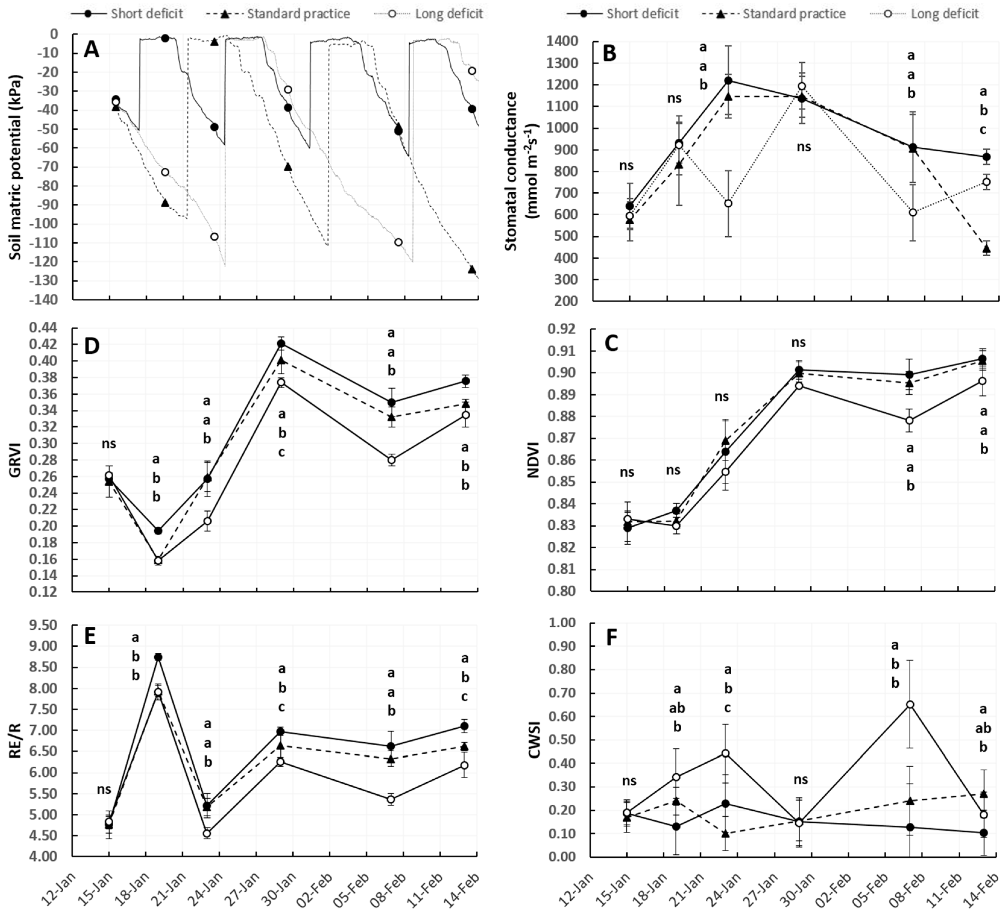
Figure 4 illustrates the mean values of soil matric potential, stomatal conductance, GRVI, NDVI, RE/R and CWSI for each irrigation treatment and measurement date during the second season of study. As obtained during the previous season, no statistically significant differences were observed between N rates in terms of stomatal conductance, NDVI, GRVI, RE/R and CWSI (data not shown).
3.2.1. Soil and Plant Water Status
During this growing season, the first images of the site were acquired on January 15 2018, prior to when separate irrigation treatments had been imposed and all the plots had similar soil matric potential readings (Figure 4A). As observed in the previous season, soil matric potential decreased between irrigation events and reached lower values in the standard and long deficit treatments than in the most frequently irrigated treatment (short deficit). However, lower soil matric potential values were obtained in all the irrigation treatments, including the short deficit, during the 2017/18 growing season than during the 2016/17. Soil matric potential during this second season reached a minimum value of −62 kPa in the short deficit treatment, −128.0 kPa in the standard practice (last measurement date) and −122.0 kPa in the long deficit treatment. Mean soil matric potential for each treatment at the time when the stomatal conductance and remote sensing measurements were taken is also indicated in Figure 4A. During this season, measurements were conducted on dates when the standard and long deficit treatments had been irrigated a few days before and thus, the short deficit was not always the treatment with the highest (less negative) soil matric potential values (see for instance matric potential values on 23, 29 January and 13 February 2018).
Mean stomatal conductance in the most frequently irrigated treatment (short deficit) ranged during the period of measurements from 641 to 1221 mmol m−2 s−1 (Figure 4B). Similar values were obtained in the standard practice treatment with the exception of the last measurement date (13 February 2018). On this date, the standard practice treatment had not been irrigated for 12 days and had lower (p < 0.05) stomatal conductance values than the other two treatments, which had been irrigated 4–5 days before (Table 1 and Table 2). In the less frequently irrigated treatment (long deficit), reductions (p < 0.05) in stomatal conductance compared to any of the other treatments were observed on three dates (23 January, 7 and 13 February 2018). On 23 January and 7 February 2018, the long deficit treatment had not been irrigated for 13–14 days and stomatal conductance was reduced, by 47% and 33%, respectively, with respect to the short deficit treatment. On 13 February 2018, when senescence was already evident in leaves from the long deficit treatment, stomatal conductance was lower in this treatment than in the short deficit in spite of having similar soil matric potential values (both treatments had been irrigated 4–5 days before) (Figure 4A,B).
3.2.2. Multispectral Indices and CWSI
Similar to that observed during the previous season, the indices NDVI, GRVI and RE/R followed a similar trend, although in this case the multispectral indices performed differently on the second measurement date (Figure 4C–E). On this date (19 January 2018), NDVI slightly increased in the short deficit treatment while the GRVI decreased and the RE/R notably increased with respect to the previous measurement. Mean NDVI in the short deficit treatment ranged from 0.83 to 0.90 during the period of measurements. In this treatment and for the same period, mean GRVI and RE/R ranged, respectively, from 0.20 to 0.42 and from 4.70 to 8.75. The short deficit and standard practice treatments had similar values of NDVI during the study. The long deficit treatment had lower NDVI than the standard and short treatments although differences became statistically significant only on the last measurement dates on 7 and 13 February 2018 (Figure 4C). Differences in GRVI and RE/R among irrigation treatments were greater than those compared with NDVI. With the exception of the first measurement date when irrigation treatments had not been imposed yet and all the plots had a similar soil and plant water status, the less frequently irrigated treatment (long deficit) had the lowest values of GRVI and RE/R during the period of measurements (Figure 4D,E). Differences in GRVI and RE/R between the long and short deficit treatments were statistically significant on all dates. The GRVI and RE/R measurements in the standard practice treatment fluctuated according to the soil water status during this season. At the end of the period of measurements, the standard practice treatment had intermediate values of the GRVI and RE/R compared to the short and long deficit treatments.
Regarding the CWSI, mean values obtained for the most frequently irrigated treatment (short deficit) were ≤ 0.23 during the whole period of measurements (Figure 4F). CWSI in the standard practice was similar to that of the short deficit (≤ 0.27) although statistically significant differences were observed between these two treatments on 23 January and 13 February 2018. On 23 January 2018, the standard practice, which had been irrigated two days before and had the highest soil matric potential, was the treatment with the lowest CWSI. On 13 February 2018, the standard practice had the lowest values of soil matric potential recorded during this season and CWSI in this treatment was higher than in the short deficit treatment. The CWSI in the long deficit treatment increased on the first three measurement dates as soil matric potential decreased and then returned to similar values as the short deficit treatment after an irrigation event (Figure 4F). The highest CWSI value reached in this treatment, 0.65, was obtained on 7 February 2018 when the short deficit treatment had a mean CWSI of 0.13.
3.3. Relationships Between Multispectral Indices and CWSI with Soil Matric Potential and Stomatal Conductance
During the first season of study, NDVI was well correlated (p < 0.05) with soil matric potential and stomatal conductance on the last two measurement dates (3 and 8 February 2017). The GRVI and RE/R were well correlated (p < 0.05) with soil and plant water status on 16 January, 3 and 8 February 2017, when the long deficit treatment had the lowest values for both soil matric potential and stomatal conductance (Table 4). Within these dates, NDVI had generally the lowest coefficient of determination (r2). The GRVI and RE/R performed similarly in predicting soil matric potential and stomatal conductance.
In 2018, the multispectral indices correlated (p < 0.05) well with soil matric potential on 19, 23 January and 7 February 2018 (Table 4). No correlation was found on the first and fourth measurement dates (15 and 29 January), when all the treatments had similar soil water status, and the last measurement date (13 February), when the long deficit treatment had the highest soil matric potential but the lowest values of NDVI, GRVI and RE/R (Figure 4). Results obtained for the relationships between soil matric potential and the CWSI showed that good correlations (r2 > 0.76; p < 0.05) were obtained on 23 January and 7 February 2018 but not on the second measurement date (19 January) as it was observed for the GRVI and RE/R (Table 4).
Good correlations for the relationship between the VIs and CWSI with the stomatal conductance were expected on dates when soil matric potential was well correlated with the indices. Nevertheless, the VIs and CWSI correlated well (r2 > 0.82; p < 0.001) with stomatal conductance on 23 January and 7 February but not on 19 January (Table 4), when no differences in stomatal conductance were observed among treatments in spite of the notable differences in soil matric potential (Figure 4A,B). Additionally, a good correlation was also found between the stomatal conductance and the CWSI (not the multispectral indices) on the last measurement date (13 February 2018) when symptoms of senescence were starting to be evident in plants from the standard and particularly the long deficit treatment.
3.4. Lint Yield, Fibre Quality and Their Relationships with the Multispectral Indices and CWSI
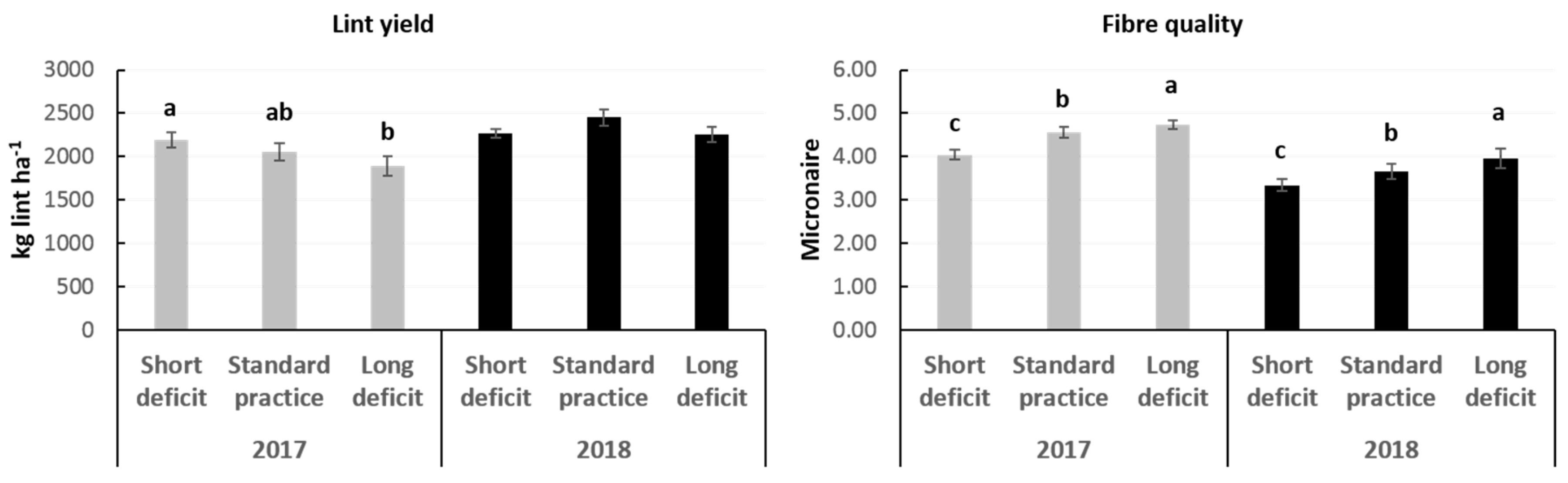
During the first season of study, irrigation frequency had a statistically significant effect (p < 0.001) on lint yield. Average lint yield in the most frequently irrigated treatment (short deficit) was 2193 kg ha−1 (Figure 5). In the long deficit treatment, lint yield was 14% lower than in the short deficit treatment. The standard practice treatment produced 6% less lint than the short deficit treatment although differences between these treatments and between the standard practice and the long deficit treatment were not statistically significant. During the 2017/18 season, lint yield in all the treatments was slightly higher than in the previous year. Frequency of irrigation did not have a statistically significant effect on lint yield. Average lint yield obtained in the short deficit treatment was 2267 kg ha−1 (Figure 5). Similar lint yield was obtained in the less frequently irrigated treatments, standard practice and long deficit.
There was a statistically significant effect of irrigation frequency on fibre micronaire in both seasons. Less frequent irrigation in the standard practice and long deficit treatments than in the short deficit had an increasing effect on micronaire (Figure 5). Micronaire in the short deficit treatment was on average 4.04 and 3.34 in 2017 and 2018, respectively. In the long deficit treatment, average values of micronaire obtained during the first and second seasons of study were 4.73 and 3.96, respectively. Intermediate values were obtained in the standard practice treatment.
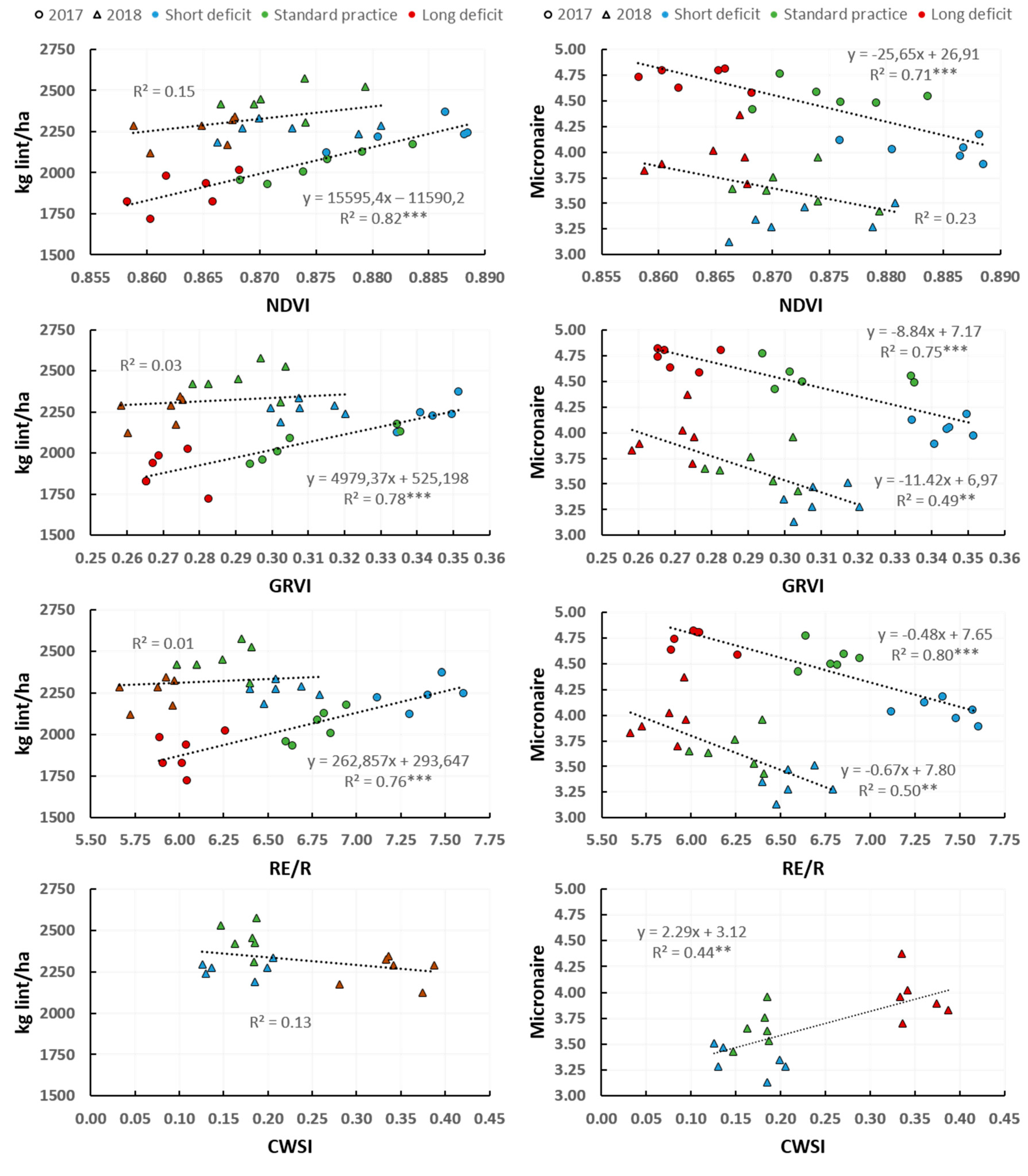
The relationship between lint yield and fibre micronaire with the VIs and CWSI was studied at the subplot level (n = 18). During the first year of study, when lint yield was significantly affected by the irrigation frequency treatments, a linear and good correlation (p < 0.001) was found between lint yield and mean NDVI, GRVI and RE/R (CWSI was not obtained this season) for all measurement dates (Figure 6). Among the VIs, NDVI had the best correlation (r2 = 0.85) while the GRVI and RE/R performed similarly in predicting yield. Different results were obtained during the second year of study. In 2018, NDVI and CWSI were poorly correlated with lint yield (Figure 6) while the GRVI and RE/R were not correlated with yield. Contrary to that observed for the lint yield, a negative correlation was observed between micronaire and mean NDVI, GRVI and RE/R for the measurement dates in both growing seasons (Figure 6). However, better correlations were obtained for all the VIs during the first year of study (r2 from 0.68 to 0.80; p < 0.001) than during the second (r2 from 0.17 to 0.49). In this case, the GRVI and RE/R performed better than the NDVI in predicting the effects of water stress on micronaire. A positive correlation (r2 = 0.45; p < 0.01) was also found in 2018 between the CWSI and micronaire.
4. Discussion
Longer intervals between irrigations in the standard (approximately every two weeks) and especially in the long deficit treatment (up to 18 days in the 2016/17 growing season) than in the treatment irrigated weekly led the plants from the former treatments to deplete the soil water profile to a higher extent than in the short deficit treatment (Figure 3A and Figure 4A). The soil water deficit experienced in the less frequently irrigated treatments led these plants to suffer a temporal reduction of the stomatal conductance as has been reported in other studies on cotton [3,41], which generally returned to similar values as those obtained in the most frequently irrigated treatment after an irrigation event. Two exceptions were found in 2018 when the stomatal conductance measurements were not in accordance with the soil matric potential readings. The first exception was observed on 19 January 2018, when the stomatal conductance measurements did not reflect the large differences in soil matric potential observed among treatments (see Figure 4A,B). Although there is not a clear explanation for this, it could be related to the fact that as a non-automated and time-consuming method, the stomatal conductance measurements are usually conducted on a few plants (6–8 plants per plot in this study), which in the case of large areas may not be representative of the current water status of the crop. This has been also reported in studies comparing water stress detection methods in cotton and vineyards [49,50] and is the reason why methods such as the aerial remote sensing of crops that enable larger areas to be monitored are presented as more appropriate. Indeed, as discussed later in this section, all the indices used here with the exception of the NDVI detected differences between treatments on this date. The second case was the last measurement date in 2018 (13 February) when the long and short deficit treatments had similar soil matric potential values (had been irrigated 4–5 days before the measurements took place) but a lower (p < 0.05) stomatal conductance was observed in the long deficit treatment. By this time of the season, symptoms of senescence, which is accompanied by a drop in daily water use, were already evident in the long deficit treatment and started to show up in the standard practice. Results obtained for the stomatal conductance on this date, 13 February 2018, indicate that the difference between the short and the long deficit treatments was not caused by a lower soil water content in the long deficit treatment but by a reduction in the plant water needs in this treatment.
4.1. Response of the UAS-Based Indices to the Irrigation Frequency
Lower frequency of irrigation in the standard and long deficit treatments had a decreasing effect on the NDVI, GRVI and RE/R and an increasing effect on the CWSI compared with the treatment irrigated weekly (short deficit). This effect was consistent in both seasons for the multispectral indices (CWSI was not measured in 2017) and was more evident for the GRVI and RE/R than for the NDVI (Figure 3 and Figure 4). The better performance of the GRVI and RE/R than the NDVI in detecting differences between irrigation treatments was probably related to the higher sensitivity of both the GRVI and RE/R to changes in the green colour of leaves and changes in vegetative canopy at full canopy cover than the NDVI. Results obtained for the GRVI are in agreement with those reported by [36] and [37]. [36] observed a decrease in the GRVI when leaves from a deciduous forest changed from bright to dark green colour as the season progressed caused by the cessation of new leaf formation first and the breakdown of chlorophylls and leaf senescence later. In [37], the GRVI was better than the NDVI in capturing changes in the colour of peanut leaves from green to yellow as the crop reached senescence. In our study, the difference in foliage colour observed across the season was most likely due to differences in leaf water content between treatments rather than to differences in the chlorophyll content. Reflectance of dehydrating leaves has been reported to increase in the visible region [51]. Moreover, leaf water content has been shown to affect the relationships between chlorophyll/spectral indices and chlorophyll content in thin and moderately thick leaves [31], such as those of cotton. The authors of [31] showed that the chlorophyll indices they used in a study aimed to assess the relationships between spectral indices and leaf pigment content estimated higher chlorophyll levels in low water content leaves than in moderately high water content leaves. In our study, as previously mentioned, less frequent irrigation had a significant decreasing effect on the chlorophyll-sensitive index RE/R. Since this index is inversely related with the chlorophyll content (see [28]), these results would suggest that the standard practice and long deficit treatments had a higher chlorophyll content than the short deficit treatment. Although the chlorophyll content was not determined in this study, analysis of plant samples taken from all the subplots in February showed that at this stage there were no statistically significant differences in total plant nitrogen content among treatments, thus differences in the chlorophyll content were not expected (data not shown). These results as well as other agronomic aspects (plant biomass, number of bolls, plant nitrogen uptake and maturity among others) assessed at this site during the 2016/17 and 2017/18 growing seasons will be included in a future publication. The RE/R measurements would suggest then that differences between treatments were related to differences in leaf water content instead of differences in chlorophyll content. This result has important implications, for instance, when attempting to remotely monitor the crop nitrogen status in cotton from the first square to first flowering stages for nitrogen fertiliser recommendations by means of chlorophyll-sensitive VIs such as the RE/R. Images taken at dates with the crop at different plant water statuses would produce misleading results, because the effect of water status on the indices obscures the effect of nitrogen status. Apart from the leaf water content, differences in GRVI and RE/R among treatments could also be related to an increase in the anthocyanin levels in the less frequently irrigated treatments This has been reported for cotton under severe water restrictions as a photoprotective response to water stress [4]. In this study, we did not determine anthocyanin levels to corroborate this and future investigation on this matter would be recommended.
Results obtained for the time series of the multispectral indices in 2018 indicate that the GRVI and RE/R were able to reflect actual differences in soil water status when the water stress experienced by plants was mild (according to the stomatal conductance measurements) and did not have a permanent effect on the canopy reflectance. This was observed in the second year of the experiment for the standard practice treatment (Figure 4A,D,E). Different results were obtained for the standard practice in 2017 and for the long deficit treatment in both seasons, when lower (p < 0.05) GRVI and RE/R values than in the short treatment were constantly obtained in the less frequently irrigated treatments after the imposition of the irrigation treatments regardless of the soil water status (Figure 3 and Figure 4). In this case, the multispectral indices were most likely displaying the effects of cumulative water stress on plants. Similar results have been reported for the NDVI and the chlorophyll-sensitive index TCARI/OSAVI (the ratio of the Transformed Chlorophyll Absorption Index and the Optimized Soil-Adjusted Vegetation Index) from a single flight campaign conducted in a study on a rain-fed vineyard [52]. Authors of [52] suggested that these indices were probably reflecting a long-term response of plants to water deficit. Both green and red reflectance are affected by the total green biomass present in the crop [35], and therefore, a reduction in plant growth as a consequence of water stress will be reflected by VIs using information from these bands (such as the NDVI, GRVI and RE/R in this study) if not compensated somehow.
As expected and in agreement with [52], the CWSI was in accordance with the actual soil and plant water status of the treatments and an irrigation event always returned the less frequently irrigated treatments to similar CWSI values of those of the short deficit treatment (Figure 4F). Recommended CWSI thresholds have been reported for the flowering, boll filling and defoliation stages in cotton [49]. In our study, Tc measurements were conducted during the flowering and early boll filling stages. During this period, the CWSI for the standard and short deficit treatments ranged within the recommended CWSI thresholds reported in [49] (0.25–0.43 and 0.30–0.65 for the flowering and boll filling stages, respectively). In the long deficit treatment, CWSI measurements surpassed the recommended thresholds on 7 February 2018 (0.67 ± 0.18), when this treatment had not been irrigated for 14 days.
4.2. Performance of the UAS-Based Indices to Predict Soil Matric Potential and Cotton Water Status
The relationships between the VIs and CWSI with the soil matric potential and stomatal conductance also support the suggestion that the multispectral indices displayed long-term effects of water stress on plants. Significant and high correlations were observed between all the indices studied and the soil and plant water status on specific dates during the study. Exceptions for this in the case of the multispectral indices were found on one measurement date in 2017 and 2–3 dates in 2018 (measurements on 15 January, 2018 when irrigation treatments had not been imposed yet is not taken into account). In 2017, the exception was found on January 27, when the long deficit treatment had intermediate values of soil matric potential and stomatal conductance but it was the treatment with the lowest values of NDVI, GRVI and RE/R along with the standard practice treatment. Similar results were observed in 2018 on 29 January and 13 February, when in spite of having the highest soil matric potential (wettest soil) the long deficit treatment had the lowest values of NDVI, GRVI and RE/R. This was most likely because the multispectral indices were reflecting effects of the water stress suffered on previous dates on this treatment, thus hampering their use for determinations of the actual soil and plant water status. No correlations were observed either between the multispectral indices and the stomatal conductance on 19 January 2018. This was also the case for the CWSI measurements. The stomatal conductance measurements on this date did not capture the existing differences in plant water status among treatments while the GRVI, RE/R and CWSI did (Figure 4D–F).
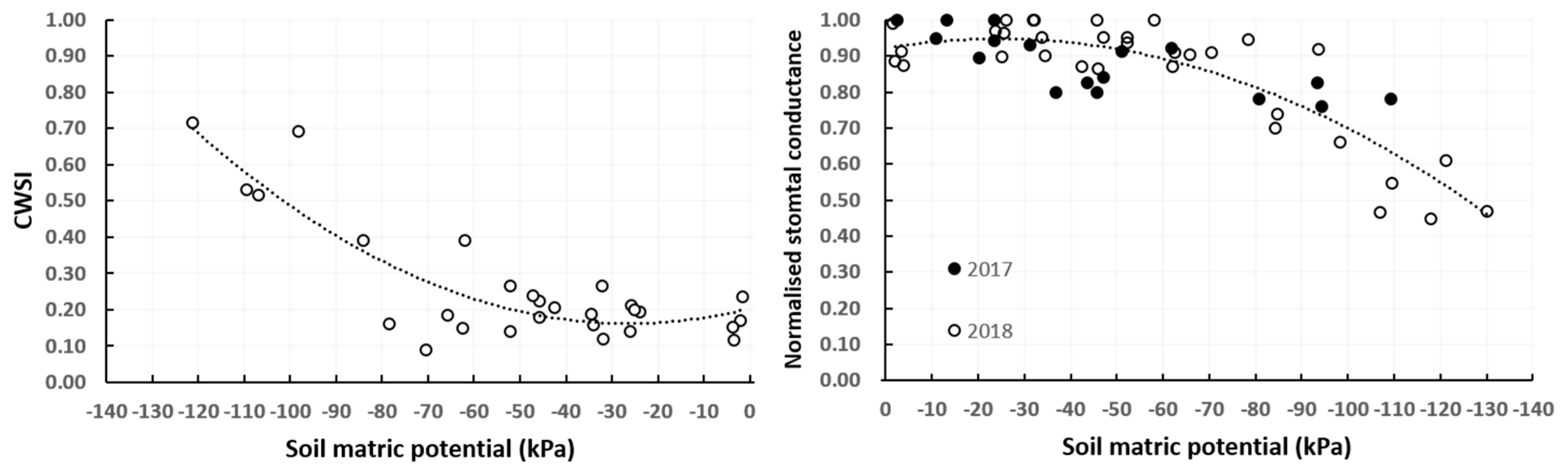
Thus, although GRVI and RE/R measurements have been shown in this study to be capable of tracking the effects of water stress on cotton, for determinations of the actual soil and plant water status (particularly late in the season), the use of the CWSI was a more robust indicator of water stress. Plotting the CWSI measurements taken in 2018 with the soil matric potential readings, it is shown that the CWSI did not change until the soil dried to a value of −50 kPa (Figure 7). It was around that value of soil matric potential (−50 to −60 kPa) when the stomatal conductance of the fifth leaf below the terminal, where these measurements were conducted, started to decline in this study (Figure 7). This result would be in agreement with results obtained in [41], in which the authors observed a non-linear relationship between the CWSI and the fraction of transpirable soil water (FTSW) with no changes in CWSI until the soil dried to FTSW values of 0.4–0.5.
4.3. Lint Yield and Lint Quality Prediction
In agreement with most of the literature existing on the use of VIs for lint yield prediction [25,53,54], the NDVI was a better predictor of the effects of water stress on lint yield than the pigment-related indices GRVI and RE/R. This is attributed to the direct relationship in cotton between plant biomass and lint yield [55].
The GRVI and RE/R were better predictors of the effects of water stress on micronaire than the NDVI. This was most likely because water stress during boll filling has detrimental effects on fibre quality and both the GRVI and RE/R were more sensitive to soil and plant water status than the NDVI. Variability in plant water status in a cotton field can then lead to a large variability in fibre quality, reducing the chances of cotton producers to meet the quality standards to achieve micronaire premium prices or even worst, incurring discounts for low micronaire. Results obtained from this study suggest that UAS-based and potentially satellite-based GRVI and RE/R measurements could be useful to estimate fibre quality during the boll filling stage. This would be of great value for cotton producers, who, in the case of large variability, could then decide whether to harvest the entire field at once or segregate the harvest by zones in order to manage that variability, which in some studies has been shown as economically justifiable [39].
Different results between seasons in yield and micronaire prediction could be related to the fact that cotton was sown earlier (14 days) and the frequency irrigation treatments started later (8 days) during the second season of study (2017/18) than during the 2016/17 season. Thus, the crop was more advanced in 2018 than in 2017 when plants experienced soil water deficit in the standard and long deficit treatments. Cotton lint yield and fiber quality are more affected by water stress early in the season (flowering) than later and thus, the better yield and micronaire prediction observed for the 2016/17 growing season than for the 2017/18 could be related to differences between seasons in the crop stage at the moment when plants experienced water stress. The lower soil matric potential values reached in the short deficit treatment during the second season of study (values around −60 kPa) than in the first season (values < −40 kPa) could have also contributed to the different results obtained between seasons.
5. Conclusions
Multispectral and thermal UAS-based imagery was used in this study to monitor the variability in soil and plant water status of a commercial cotton farm by means of the NDVI, GRVI, RE/R and CWSI. The NDVI, GRVI and RE/R decreased in response to soil water deficit and water stress, and this reduction was more marked in the GRVI and RE/R than in the NDVI. This decrease in GRVI and RE/R was most likely due to differences in leaf water content among irrigation treatments, which led to differences in foliage colour. Both the GRVI and RE/R were able to track the effects of water stress on cotton plants and were good indicators of the actual soil and plant water status when the water stress experienced by the plants did not lead to permanent changes in canopy reflectance. This was the case of the long deficit treatment in both years of study and the standard practice in the first growing season. Thus, these results suggest that for determinations of the actual soil and plant water status it is more recommendable the use of the CWSI than the multispectral indices here assessed. In this study, reductions in stomatal conductance and an increase in the CWSI were not observed until the soil dried to −50–−60 kPa, which corresponded with a CWSI value of 0.20.
The NDVI was shown as a better predictor of lint yield than the GRVI and RE/R but the opposite was found for the micronaire prediction. Both the GRVI and RE/R correlated with micronaire in both years of study. These results present the GRVI and RE/R as possible indices to be used from UASs or potentially from satellite platforms for fibre quality estimations in cotton fields. Fibre quality maps at boll filling stage would provide the cotton producers with a valuable tool to decide whether strategies such as harvest separation by zones is justify or not to manage fibre quality variability. Further research on this topic would provide more insights on the capability of these spectral indices for fibre quality monitoring in the field. Although the GRVI and RE/R performed similarly in tracking the effects of water stress and predicting lint quality, the suitability of the GRVI for filtering most of the soil background from the images (GRVI < 0) probably makes this a more useful index for crop monitoring than the RE/R. Further research is needed to evaluate the capability of these indices obtained from satellite platforms and to study whether these results obtained for cotton can be extrapolated to other crops.
Author Contributions
In-field measurements, C.B. and W.C.Q.; experimental design, W.C.Q., J.H. and C.B.; acquisition of multispectral and thermal images, C.B., J.B. and J.H.; image processing, C.B. and J.B.; data analysis, C.B.; writing—original draft preparation, C.B.; writing—review and editing, J.B., W.C.Q., J.H.; funding acquisition, W.C.Q. and J.H.
Funding
This research was funded by the Australian Department of Agriculture and Water Resources, Rural R&D for Profit Programme Round 1, Maximising On-Farm Irrigation Profitability Project. Grant No. RnD4Profit-14-01 2015-2018.
Acknowledgments
The authors are thankful for the great assistance provided by Mr. James Hill and Mr. Matt Watson, agronomists of the site where this study was conducted and the Stott Agricultural Company.
Conflicts of Interest
The authors declare no conflict of interest. The funders had no role in the design of the study; in the collection, analyses, or interpretation of data; in the writing of the manuscript, or in the decision to publish the results.
References
- Alvino, A.; Marino, S. Remote sensing for irrigation of horticultural crops. Horticulturae 2017, 3, 40. [Google Scholar]
- Osakabe, Y.; Osakabe, K.; Shinozaki, K.; Tran, L.-S. Response of plants to water stress. Front. Plant Sci. 2014, 5, 86. [Google Scholar] [CrossRef]
- Baker, J.T.; Gitz, D.C.; Payton, P.; Wanjura, D.F.; Upchurch, D.R. Using leaf gas exchange to quantify drought in cotton irrigated based on canopy temperature measurements. Agron. J. 2007, 99, 637–644. [Google Scholar] [CrossRef]
- Deeba, F.; Pandey, A.K.; Ranjan, S.; Mishra, A.; Singh, R.; Sharma, Y.K.; Shirke, P.A.; Pandey, V. Physiological and proteomic responses of cotton (gossypium herbaceum l.) to drought stress. Plant Physiol. Biochem. 2012, 53, 6–18. [Google Scholar] [CrossRef]
- Wiggins, M.S.; Leib, B.G.; Mueller, T.C.; Main, C.L. Cotton growth, yield, and fiber quality response to irrigation and water deficit in soil of varying depth to a sand layer. J. Cotton Sci. 2014, 18, 145–152. [Google Scholar]
- Brodrick, R.; Yeates, S.; Roth, G.; Gibb, D.; Henggeler, S.; Wigginton, D. Managing irrigated cotton agronomy. In Waterpak—A Guide for Irrigation Management in Cotton and Grain Farming Systems; Dugdale, H., Harris, G., Neilsen, J., Richards, D., Wigginton, D., Williams, D., Eds.; The Cotton Research and Development Corporation: Narrabri, Australia, 2012; pp. 248–263. [Google Scholar]
- Bange, M.P.; Constable, G.A.; Gordon, S.G.; Naylor, M.H.J. Van der Sluijs. In Fibrepak a Guide to Improving Australian Cotton Fibre Quality; The Cotton Research and Development Corporation: Narrabri, Australia, 2009. [Google Scholar]
- Fernández, J. Plant-based methods for irrigation scheduling of woody crops. Horticulturae 2017, 3, 35. [Google Scholar] [CrossRef]
- Ihuoma, S.O.; Madramootoo, C.A. Recent advances in crop water stress detection. Comput. Electron. Agric. 2017, 141, 267–275. [Google Scholar] [CrossRef]
- Cohen, Y.; Alchanatis, V.; Meron, M.; Saranga, Y.; Tsipris, J. Estimation of leaf water potential by thermal imagery and spatial analysis*. J. Exp. Bot. 2005, 56, 1843–1852. [Google Scholar] [CrossRef] [PubMed]
- Ko, J.; Piccinni, G. Characterizing leaf gas exchange responses of cotton to full and limited irrigation conditions. Field Crop. Res. 2009, 112, 77–89. [Google Scholar] [CrossRef]
- Cohen, Y.; Fuchs, M.; Falkenflug, V.; Moreshet, S. Calibrated heat pulse method for determining water uptake in cotton. Agron. J. 1988, 80, 398–402. [Google Scholar] [CrossRef]
- Cohen, Y.; Alchanatis, V.; Saranga, Y.; Rosenberg, O.; Sela, E.; Bosak, A.J.P.A. Mapping water status based on aerial thermal imagery: Comparison of methodologies for upscaling from a single leaf to commercial fields. Precis. Agric. 2017, 18, 801–822. [Google Scholar] [CrossRef]
- Jones, H.G.; Serraj, R.; Loveys, B.R.; Xiong, L.; Wheaton, A.; Price, A.H. Thermal infrared imaging of crop canopies for the remote diagnosis and quantification of plant responses to water stress in the field. Funct. Plant Biol. 2009, 36, 978–989. [Google Scholar] [CrossRef]
- Idso, S.B.; Jackson, R.D.; Pinter, P.J.; Reginato, R.J.; Hatfield, J.L. Normalizing the stress-degree-day parameter for environmental variability. Agric. Meteorol. 1981, 24, 45–55. [Google Scholar] [CrossRef]
- Jackson, R.D.; Idso, S.B.; Reginato, R.J.; Pinter, P.J. Canopy temperature as a crop water stress indicator. Water Resour. Res. 1981, 17, 1133–1138. [Google Scholar] [CrossRef]
- Meron, M.; Tsipris, J.; Orlov, V.; Alchanatis, V.; Cohen, Y.J.P.A. Crop water stress mapping for site-specific irrigation by thermal imagery and artificial reference surfaces. Precis. Agric. 2010, 11, 148–162. [Google Scholar] [CrossRef]
- Bellvert, J.; Zarco-Tejada, P.J.; Girona, J.; Fereres, E.J.P.A. Mapping crop water stress index in a ‘pinot-noir’ vineyard: Comparing ground measurements with thermal remote sensing imagery from an unmanned aerial vehicle. Precis. Agric. 2014, 15, 361–376. [Google Scholar] [CrossRef]
- Gonzalez-Dugo, V.; Zarco-Tejada, P.; Nicolás, E.; Nortes, P.A.; Alarcón, J.J.; Intrigliolo, D.S.; Fereres, E.J.P.A. Using high resolution uav thermal imagery to assess the variability in the water status of five fruit tree species within a commercial orchard. Precis. Agric. 2013, 14, 660–678. [Google Scholar] [CrossRef]
- Matese, A.; Baraldi, R.; Berton, A.; Cesaraccio, C.; Di Gennaro, S.; Duce, P.; Facini, O.; Mameli, M.; Piga, A.; Zaldei, A. Estimation of water stress in grapevines using proximal and remote sensing methods. Remote Sens. 2018, 10, 114. [Google Scholar] [CrossRef]
- Govender, M.; Govender, P.G.; Weiersbye, I.M.; Witkowski, E.T.F.; Ahmed, F. Review of commonly used remote sensing and ground-based technologies to measure plant water stress. Water Sa 2009, 35, 741–752. [Google Scholar] [CrossRef]
- Haise, H.R.; Hagan, R.M. Soil, plant, and evaporative measurements as criteria for scheduling irrigation1. In Irrigation of Agricultural Lands; Hagan, R.M., Haise, H.R., Edminster, T.W., Eds.; American Society of Agronomy: Madison, WI, USA, 1967; pp. 577–604. [Google Scholar]
- Zarco-Tejada, P.J.; Miller, J.R.; Mohammed, G.H.; Noland, T.L.; Sampson, P.H. Chlorophyll fluorescence effects on vegetation apparent reflectance: II. Laboratory and airborne canopy-level measurements with hyperspectral data. Remote Sens. Environ. 2000, 74, 596–608. [Google Scholar] [CrossRef]
- Ju, C.-H.; Tian, Y.-C.; Yao, X.; Cao, W.-X.; Zhu, Y.; Hannaway, D. Estimating leaf chlorophyll content using red edge parameters. Pedosphere 2010, 20, 633–644. [Google Scholar] [CrossRef]
- Ballester, C.; Hornbuckle, J.; Brinkhoff, J.; Smith, J.; Quayle, W. Assessment of in-season cotton nitrogen status and lint yield prediction from unmanned aerial system imagery. Remote Sens. 2017, 9, 1149. [Google Scholar] [CrossRef]
- Frampton, W.J.; Dash, J.; Watmough, G.; Milton, E.J. Evaluating the capabilities of sentinel-2 for quantitative estimation of biophysical variables in vegetation. ISPRS J. Photogramm. Remote Sens. 2013, 82, 83–92. [Google Scholar] [CrossRef]
- Raper, T.B.; Varco, J.J.; Hubbard, K.J. Canopy-based normalized difference vegetation index sensors for monitoring cotton nitrogen status. Agron. J. 2013, 105, 1345–1354. [Google Scholar] [CrossRef]
- Ballester, C.; Zarco-Tejada, P.J.; Nicolás, E.; Alarcón, J.J.; Fereres, E.; Intrigliolo, D.S.; Gonzalez-Dugo, V.J.P.A. Evaluating the performance of xanthophyll, chlorophyll and structure-sensitive spectral indices to detect water stress in five fruit tree species. Precis. Agric. 2018, 19, 178–193. [Google Scholar] [CrossRef]
- Blackburn, G.A. Hyperspectral remote sensing of plant pigments. J. Exp. Bot. 2007, 58, 855–867. [Google Scholar] [CrossRef]
- Gamon, J.A.; Peñuelas, J.; Field, C.B. A narrow-waveband spectral index that tracks diurnal changes in photosynthetic efficiency. Remote Sens. Environ. 1992, 41, 35–44. [Google Scholar] [CrossRef]
- Sims, D.A.; Gamon, J.A. Relationships between leaf pigment content and spectral reflectance across a wide range of species, leaf structures and developmental stages. Remote Sens. Environ. 2002, 81, 337–354. [Google Scholar] [CrossRef]
- Zarco-Tejada, P.J.; Miller, J.R.; Morales, A.; Berjón, A.; Agüera, J. Hyperspectral indices and model simulation for chlorophyll estimation in open-canopy tree crops. Remote Sens. Environ. 2004, 90, 463–476. [Google Scholar] [CrossRef]
- Inoue, Y.; Peñuelas, J.; Miyata, A.; Mano, M. Normalized difference spectral indices for estimating photosynthetic efficiency and capacity at a canopy scale derived from hyperspectral and co2 flux measurements in rice. Remote Sens. Environ. 2008, 112, 156–172. [Google Scholar] [CrossRef]
- Maimaitiyiming, M.; Ghulam, A.; Bozzolo, A.; Wilkins, J.L.; Kwasniewski, M.T. Early detection of plant physiological responses to different levels of water stress using reflectance spectroscopy. Remote Sens. 2017, 9, 745. [Google Scholar] [CrossRef]
- Tucker, C.J. Red and photographic infrared linear combinations for monitoring vegetation. Remote Sens. Environ. 1979, 8, 127–150. [Google Scholar] [CrossRef]
- Motohka, T.; Nasahara, K.N.; Oguma, H.; Tsuchida, S. Applicability of green-red vegetation index for remote sensing of vegetation phenology. Remote Sens. 2010, 2, 2369–2387. [Google Scholar] [CrossRef]
- Chen, A.; Orlov-Levin, V.; Meron, M. Applying high-resolution visible-channel aerial scan of crop canopy to precision irrigation management. Proceedings 2018, 2, 335. [Google Scholar] [CrossRef]
- Cotton Australia. Available online: https://cottonaustralia.com.au/cotton-library/fact-sheets/cotton-fact-file-the-australian-cotton-industry (accessed on 4 December 2018).
- Wang, R.; Thomasson, J.A.; Cox, M.S.; Sui, R.; Hollingsworth, E.G.M. Cotton fiber-quality prediction based on spatial variability in soils. J. Cotton Sci. 2017, 21, 220–228. [Google Scholar]
- Ge, Y.; Thomasson, J.A.; Sui, R.; Morgan, C.L.; Searcy, S.W.; Parnell, C.B.J.P.A. Spatial variation of fiber quality and associated loan rate in a dryland cotton field. Precis. Agric. 2008, 9, 181–194. [Google Scholar] [CrossRef]
- Lacape, M.J.; Wery, J.; Annerose, D.J.M. Relationships between plant and soil water status in five field-grown cotton (Gossypium hirsutum L.) cultivars. Field Crop. Res. 1998, 57, 29–43. [Google Scholar] [CrossRef]
- Jackson, R.D. Canopy temperature and crop water stress. In Advances in Irrigation; Hillel, D., Ed.; Elsevier: Amsterdam, Netherlands, 1982; Volume 1, pp. 43–85. [Google Scholar]
- Zarco-Tejada, P.J.; González-Dugo, V.; Berni, J.A.J. Fluorescence, temperature and narrow-band indices acquired from a uav platform for water stress detection using a micro-hyperspectral imager and a thermal camera. Remote Sens. Environ. 2012, 117, 322–337. [Google Scholar] [CrossRef]
- Isbell, R.F. The Australian Soil Classification; CSIRO: Collingwood, Australia, 2002. [Google Scholar]
- Brinkhoff, J.; Hornbuckle, J.; Quayle, W.; Lurbe, C.B.; Dowling, T. Wifield, an IEEE 802.11-based agricultural sensor data gathering and logging platform. In Proceedings of the 2017 Eleventh International Conference on Sensing Technology (ICST), Sydney, Australia, 4–6 December 2017; pp. 1–6. [Google Scholar]
- Meron, M.; Alchanatis, V.; Cohen, Y.; Tsipris, J. Aerial thermography for crop stress evaluation—A look into the state of the technology. In Precision Agriculture ’13; Stafford, J.V., Ed.; Wageningen Academic Publishers: Wageningen, The Netherlands, 2013; pp. 177–183. [Google Scholar]
- Rouse, J.W.H.; Haas, R.H.; Schell, J.A.; Deering, D.W. Monitoring vegetation systems in the great plains with ERTS. In Proceedings of the Third Earth Resources Technology Satellite-1 Symposium, Washington, DC, USA, 10–14 December 1973; Freden, S.C., M.E.P., Becker, M.A., Eds.; 1974; pp. 309–317. [Google Scholar]
- Ballester, C.; Jiménez-Bello, M.A.; Castel, J.R.; Intrigliolo, D.S. Usefulness of thermography for plant water stress detection in citrus and persimmon trees. Agric. For. Meteorol. 2013, 168, 120–129. [Google Scholar] [CrossRef]
- Cohen, Y.; Alchanatis, V.; Sela, E.; Saranga, Y.; Cohen, S.; Meron, M.; Bosak, A.; Tsipris, J.; Ostrovsky, V.; Orolov, V.; et al. Crop water status estimation using thermography: Multi-year model development using ground-based thermal images. Precis. Agric. 2015, 16, 311–329. [Google Scholar] [CrossRef]
- Möller, M.; Alchanatis, V.; Cohen, Y.; Meron, M.; Meron, M.; Tsipris, J.; Naor, A.; Ostrovsky, V.; Sprintsin, M.; Cohen, S. Use of thermal and visible imagery for estimating crop water status of irrigated grapevine*. J. Exp. Bot. 2006, 58, 827–838. [Google Scholar] [CrossRef]
- Aldakheel, Y.Y.; Danson, F.M. Spectral reflectance of dehydrating leaves: Measurements and modelling. Int. J. Remote Sens. 1997, 18, 3683–3690. [Google Scholar] [CrossRef]
- Baluja, J.; Diago, M.P.; Balda, P.; Zorer, R.; Meggio, F.; Morales, F.; Tardaguila, J.J.I.S. Assessment of vineyard water status variability by thermal and multispectral imagery using an unmanned aerial vehicle (uav). Irrig. Sci. 2012, 30, 511–522. [Google Scholar] [CrossRef]
- Gutierrez, M.; Norton, R.; Thorp, K.R.; Wang, G. Association of spectral reflectance indices with plant growth and lint yield in upland cotton. Crop Sci. 2012, 52, 849–857. [Google Scholar] [CrossRef]
- Zhao, D.; Reddy, K.R.; Kakani, V.G.; Read, J.J.; Koti, S. Canopy reflectance in cotton for growth assessment and lint yield prediction. Eur. J. Agron. 2007, 26, 335–344. [Google Scholar] [CrossRef]
- Rochester, I.J. Nutrient uptake and export from an australian cotton field. Nutr. Cycl. Agroecosyst. 2007, 77, 213–223. [Google Scholar] [CrossRef]
Figure 1.
Location of the commercial cotton farm at Darlington Point, NSW, Australia, where the study was conducted.
Figure 1.
Location of the commercial cotton farm at Darlington Point, NSW, Australia, where the study was conducted.

Figure 2.
Distribution of the treatments in the field. The red rectangle indicates the area used for the study presented here. The black dots indicate the monitoring stations, each with two matric potential sensors within the main plots 4, 5 and 6. Subplots with the highest nitrogen (N) rates received 277 and 309 kg N ha−1 the first and second growing seasons, respectively. Subplots with the lowest nitrogen (N) rates received 180 kg N ha−1 in the 2016/17 season and 244 kg N ha−1 in the 2017/18.

Figure 3.
Mean values of (A) soil matric potential, (B) stomatal conductance and the multispectral vegetation indices, (C) GRVI, (D) NDVI and (E) RE/R for each irrigation treatment and measurement date during the 2016/17 growing season. Graph A also shows the evolution of the soil matric potential for the period when all the measurements were taken (from 15 January to 8 February 2017). Dates when soil matric potential returns to values < −10 kPa are indicative of an irrigation event. Different letters within a measurement date indicate statistical significant differences between treatments at p < 0.05. The letter on the top refers to the highest value whereas the letter on the bottom refers to the lowest. Vertical bars indicate the standard deviation for each treatment and date.

Figure 4.
Mean values of (A) soil matric potential, (B) stomatal conductance and the multispectral vegetation indices (C) NDVI, (D) GRVI, (E) RE/R and (F) the CWSI for each irrigation treatment and measurement date during the 2017/18 growing season. Graph A also shows the evolution of the soil matric potential for the period when all the measurements were taken (from 15 January to 13 February 2018). Dates when soil matric potential returns to values < −10 kPa are indicative of an irrigation event. Different letters within a measurement date, indicate statistical significant differences between treatments at p < 0.05. The letter on the top refers to the highest value whereas the letter on the bottom refers to the lowest. No statistically significant differences are indicated by “ns”. Vertical bars indicate the standard deviation for each treatment and date.

Figure 5.
Average values of lint yield and fibre macronaire for each irrigation treatment during the 2016/17 and 2017/18 cotton growing seasons. Different letters between treatments within each season indicate statistically significant differences at p < 0.05. Vertical bars indicate the standard deviation for each treatment.

Figure 6.
Relationships between lint yield and fibre micronaire with the subplot mean NDVI, GRVI, RE/R and CWSI for all the measurement dates within each growing season. ** and *** indicate statistical significance at p < 0.01 and p < 0.001, respectively.
Figure 6.
Relationships between lint yield and fibre micronaire with the subplot mean NDVI, GRVI, RE/R and CWSI for all the measurement dates within each growing season. ** and *** indicate statistical significance at p < 0.01 and p < 0.001, respectively.

Figure 7.
Soil matric potential relationships with CWSI (left; data only for 2018, r2 = 0.74) and normalised stomatal conductance (right; r2 = 0.73).
Figure 7.
Soil matric potential relationships with CWSI (left; data only for 2018, r2 = 0.74) and normalised stomatal conductance (right; r2 = 0.73).


Table 1.
Dates when irrigation events occurred in each treatment during the period of measurements within the 2016/17 and 2017/18 seasons.
Table 1.
Dates when irrigation events occurred in each treatment during the period of measurements within the 2016/17 and 2017/18 seasons.
| Irrigation Events | ||||||
|---|---|---|---|---|---|---|
| 2016/17 | 1st | 2nd | 3rd | 4th | 5th | 6th |
| Short deficit | 2-January | 10-January | 17-January | 24-January | 29-January | 7-February |
| Standard practice | 2-January | 17-January | 29-January | - | - | - |
| Long deficit | 2-January | 21-January | - | - | - | - |
| 2017/18 | ||||||
| Short deficit | 10-January | 17-January | 24-January | 31-January | 8-February | - |
| Standard practice | 10-January | 21-January | 1-February | - | - | - |
| Long deficit | 10-January | 24-January | 9-February | - | - | - |
Table 2.
Dates when multispectral and thermal images of the site were taken with the average values for air temperature (Ta, °C), relative humidity (RH, %), solar radiation (SR, W m−2), wind speed (WS, km h−1) and vapor pressure deficit (VPD, kPa) averaged from 11 h to 15 h. The number of days since the last irrigation event for each treatment and measurement date are also indicated.
| Date of Measurements | Ta | RH | SR | WS | VPD | Long Deficit | Standard Practice | Short Deficit |
|---|---|---|---|---|---|---|---|---|
| 2017 | Days since las irrigation | |||||||
| 16 January | 34.64 | 22.69 | 993.21 | 6.28 | 4.29 | 14 | 14 | 6 |
| 27 January | 34.52 | 27.16 | 963.71 | 7.84 | 4.03 | 6 | 10 | 3 |
| 3 February | 31.32 | 26.33 | 792.40 | 5.19 | 3.38 | 13 | 5 | 5 |
| 8 February | 31.20 | 45.00 | 915.57 | 13.70 | 2.53 | 18 | 10 | 1 |
| 2018 | ||||||||
| 15 January | 27.69 | 34.02 | 974.48 | 3.13 | 2.46 | 5 | 5 | 5 |
| 19 January | 39.36 | 21.15 | 985.07 | 4.77 | 5.67 | 9 | 9 | 2 |
| 23 January | 39.06 | 27.28 | 852.99 | 11.03 | 5.12 | 13 | 2 | 6 |
| 29 January | 34.60 | 41.30 | 861.98 | 14.43 | 3.27 | 5 | 8 | 5 |
| 7 February | 36.82 | 27.46 | 928.35 | 15.14 | 4.59 | 14 | 6 | 7 |
| 13 February | 31.32 | 28.16 | 912.46 | 4.82 | 3.30 | 4 | 12 | 5 |
Table 3.
Indices calculated in the study for cotton water status monitoring obtained from UAS imagery. The band centres used in this study for computing the multispectral indices were 475, 560, 668, 717 and 840 nm for the blue, (B), green (G), red (R), red-edge (RE) and near infrared (NIR) bands, respectively.
| Vegetation Index | Formulation | Reference |
|---|---|---|
| Normalized Difference Vegetation Index (NDVI) | (NIR − R)/(NIR + R) | [47] |
| Green Red Vegetation Index (GRVI) | (G − R)/(G + R) | [35] |
| Red-edge ratio (RE/R) | RE/R | [48] |
| Crop Water Stress Index (CWSI) | *(Tc − Twet)/(Tdry − Twet) | [16] |
* According to [13]; Tc = canopy temperature; Twet = 5% coldest canopy-related pixels; Tdry = air temperature + 5°C
Table 4.
Coefficient of determination (r2) obtained for the relationship between the stomatal conductance and soil matric potential with the thermal (CWSI) and spectral indices (NDVI, GRVI and RE/R) for each measurement date.
Table 4.
Coefficient of determination (r2) obtained for the relationship between the stomatal conductance and soil matric potential with the thermal (CWSI) and spectral indices (NDVI, GRVI and RE/R) for each measurement date.
| 2016/2017 Growing Season | 2017/2018 Growing Season | ||||||||||
|---|---|---|---|---|---|---|---|---|---|---|---|
| 16/01/2017 | 27/01/2017 | 3/02/2017 | 8/02/2017 | 15/01/2018 | 19/01/2018 | 23/01/2018 | 29/01/2018 | 7/02/2018 | 13/02/2018 | ||
| Soil matric potential vs. | NDVI | 0.03 | 0.16 | 0.79 * | 0.72 * | 0.08 | 0.38 | 0.65 * | 0.02 | 0.73 * | 0.28 |
| GRVI | 0.66 * | 0.52 | 0.92 ** | 0.97 *** | 0.03 | 0.85 ** | 0.70 * | 0.01 | 0.80 * | 0.02 | |
| RE/R | 0.74 * | 0.41 | 0.85 ** | 0.89 ** | 0.00 | 0.87 ** | 0.58 | 0.00 | 0.82 * | 0.04 | |
| CWSI | - | - | - | - | 0.01 | 0.54 | 0.83 * | 0.52 | 0.76 * | 0.43 | |
| Stomatal conductance vs. | NDVI | 0.19 | 0.04 | 0.80 * | 0.85 * | 0.14 | 0.13 | 0.89 ** | 0.46 | 0.87 ** | 0.01 |
| GRVI | 0.84 * | 0.37 | 0.83 * | 0.97 ** | 0.45 | 0.12 | 0.85 ** | 0.19 | 0.89 ** | 0.10 | |
| RE/R | 0.77 * | 0.39 | 0.72 * | 0.98 ** | 0.14 | 0.07 | 0.91 ** | 0.14 | 0.91 ** | 0.07 | |
| CWSI | - | - | - | - | 0.24 | 0.00 | 0.82 * | 0.14 | 0.91 ** | 0.89 ** | |
*, ** and *** mean, respectively, statistical significance at p < 0.05, p < 0.01 and p < 0.001.
© 2019 by the authors. Licensee MDPI, Basel, Switzerland. This article is an open access article distributed under the terms and conditions of the Creative Commons Attribution (CC BY) license (http://creativecommons.org/licenses/by/4.0/).
Share and Cite
MDPI and ACS Style
Ballester, C.; Brinkhoff, J.; Quayle, W.C.; Hornbuckle, J. Monitoring the Effects of Water Stress in Cotton Using the Green Red Vegetation Index and Red Edge Ratio. Remote Sens. 2019, 11, 873. https://doi.org/10.3390/rs11070873
AMA Style
Ballester C, Brinkhoff J, Quayle WC, Hornbuckle J. Monitoring the Effects of Water Stress in Cotton Using the Green Red Vegetation Index and Red Edge Ratio. Remote Sensing. 2019; 11(7):873. https://doi.org/10.3390/rs11070873
Chicago/Turabian StyleBallester, Carlos, James Brinkhoff, Wendy C. Quayle, and John Hornbuckle. 2019. "Monitoring the Effects of Water Stress in Cotton Using the Green Red Vegetation Index and Red Edge Ratio" Remote Sensing 11, no. 7: 873. https://doi.org/10.3390/rs11070873
Note that from the first issue of 2016, this journal uses article numbers instead of page numbers. See further details here.