Article

Hierarchical Growing Neural Gas Network (HGNG)-Based Semicooperative Feature Classifier for IDS in Vehicular Ad Hoc Network (VANET)

1
Department of Electronics and Information Engineering, Huazhong University of Science and Technology, Wuhan 430074, China
2
School of Information Technology, Faculty of Science, Engineering and Built Environment, Deakin University, Geelong 3220, Australia
*
Author to whom correspondence should be addressed.
J. Sens. Actuator Netw. 2018, 7(3), 41; https://doi.org/10.3390/jsan7030041
Submission received: 8 August 2018 / Revised: 7 September 2018 / Accepted: 10 September 2018 / Published: 14 September 2018
(This article belongs to the Special Issue Vehicle Networks: State-of-the-Art and Prospects)

Abstract

:
In this research, new modeling strategy based hierarchical growing neural gas network (HGNG)-semicooperative for feature classifier of intrusion detection system (IDS) in a vehicular ad hoc network (VANET). The novel IDS mainly presents a new design feature for an extraction mechanism and a HGNG-based classifier. Firstly, the traffic flow features and vehicle location features were extracted in the VANET model. In order to effectively extract location features, a semicooperative feature extraction is used for collecting the current location information for the neighboring vehicles through a cooperative manner and the location features of the historical location information. Secondly, the HGNG-based classifier was designed for evaluating the IDS by using a hierarchy learning process without the limitation of the fix lattice topology. Finally, an additional two-step confirmation mechanism is used to accurately determine the abnormal vehicle messages. In the experiment, the proposed IDS system was evaluated, observed, and compared with the existing IDS. The proposed system performed a remarkable detection accuracy, stability, processing efficiency, and message load.

1. Introduction

Vehicle ad hoc network (VANET) is considered one of the new technologies that can dramatically change our way of life. It will significantly improve the quality of human lives and will become a reality in the near future [1,2]. Over the past three years, many vehicle designers began to incorporate wireless access in vehicular environment (WAVE) in their vehicles [3]. WAVE is a technology based on the IEEE 802.11p protocol standards which provides the basic broadcast standard for dedicated short-range communications technology (DSRC) [4]. VANET enables wireless communication among moving vehicles through the DSRC, which includes vehicle-to-vehicle communication (V2V) and vehicle infrastructure communication (V2I) [5]. With allowing vehicles to communicate with each other and helping drivers make easier decisions, VANET significantly improves the driving safety and comfort. Since VANET manages critical traffic information and its information is closely linked to human safety, it is of paramount importance to the security of VANET. To address the security issues in VANET, IDS is deployed inside each vehicle to detect internal and external security threats. Analyzing the VANET information is one of the effective ways to protect VANET and detecting unusual activities in the VANET then alerting it [6].
For addressing VANET security issues, there are many different solutions. This includes creditworthiness mechanisms [7] and data-centric trusty mechanisms [8]. The creditworthiness mechanism gives the vehicle scores according to their historical behaviors and current behaviors, so that a vehicle has a higher level of safety with higher scores and a vehicle is regarded as a suspected vehicle with lower scores. The creditworthiness mechanism refers to assigning the trust scores to other vehicles based on historical or current interaction, where the trust score indicates the creditworthiness of the vehicle in VANET [9]. According to scores, the vehicle behaviors are restricted with varying degrees. It works well in wired networks or in online systems where the vehicle has a fixed physical identity. There are various creditworthiness schemes which were proposed by [10,11]. A centralized infrastructure was proposed to deploy a reputation mechanism [10]. A decentralized infrastructure adopted to deploy a creditworthiness mechanism [11]. However, although a creditworthiness-based scheme is useful, a fatal disadvantage of this mechanism is that it is difficult to prevent a sudden attack by a trusted vehicle. It is difficult to implement in a fast-moving and rapidly changing network such as VANET because it takes a certain amount of time to establish the creditworthiness. If the fake information comes from a trusted vehicle, the creditworthiness mechanism will have no way of limiting that information.
The data-centric trusty mechanism is applied to establish a message processing center, which evaluates and broadcasts all the messages [8]. The data-centric trusty mechanism was used to discriminate abnormal behaviors by only considering shared data [12]. Another study conducted to propose a VANET model to detect and correct errors for the data which was sent by the vehicle (the model-conforming message is accepted, otherwise the message is rejected) [10]. An emergency message is relayed and the fake information is identified based on the message type and the subsequent behaviors of the vehicle sender in a study conducted by [13]. This technique is not available for emergency messages because the emergency message requires the vehicle to react quickly. However, when the number of vehicles achieves an order of magnitude, data retention and congestion, it will result in the excessive delay of message propagation. In addition, the computational complicity is costly. Raya et al. proposed an anomaly detection system and eviction mechanism [14]. The vehicle was considered as an abnormal behavior if the message sent by the vehicle did not accord with the general situation. Once the vehicle is classified as an attacking vehicle, the neighbor’s vehicle can temporarily deport it by sharing the warning message. Subsequently, its certificate was sent to a certificate authority (CA), which revoked the fraudulent vehicle by adding it to the revocation list (RL). Unfortunately, it is difficult to manage RL in VANET.
In IDS, unlike the previous two technologies, offers a solution to VANET security issues by effectively detects attacks by analyzing and classifying the messages in the VANET. IDS accurately detects known attacks and attempts to predict new types of attacks and protect the system from unknown attacks as well [15]. However, in this intrusion prediction system, the probability threshold needs to be set sensitively to obtain accurate results.
There are some very serious security issues that need to be resolved before using IDS to prevent attacks in VANET including:
  • It is not possible to use IDS in a wired network because of its wireless and mobile nature and its dynamic topology.
  • Unlike wired networks (some of these known databases, such as NSL-KDD and KDD 99), there is no universally accepted database available for VANET. Which means IDS can only work with locally monitored data in VANET.
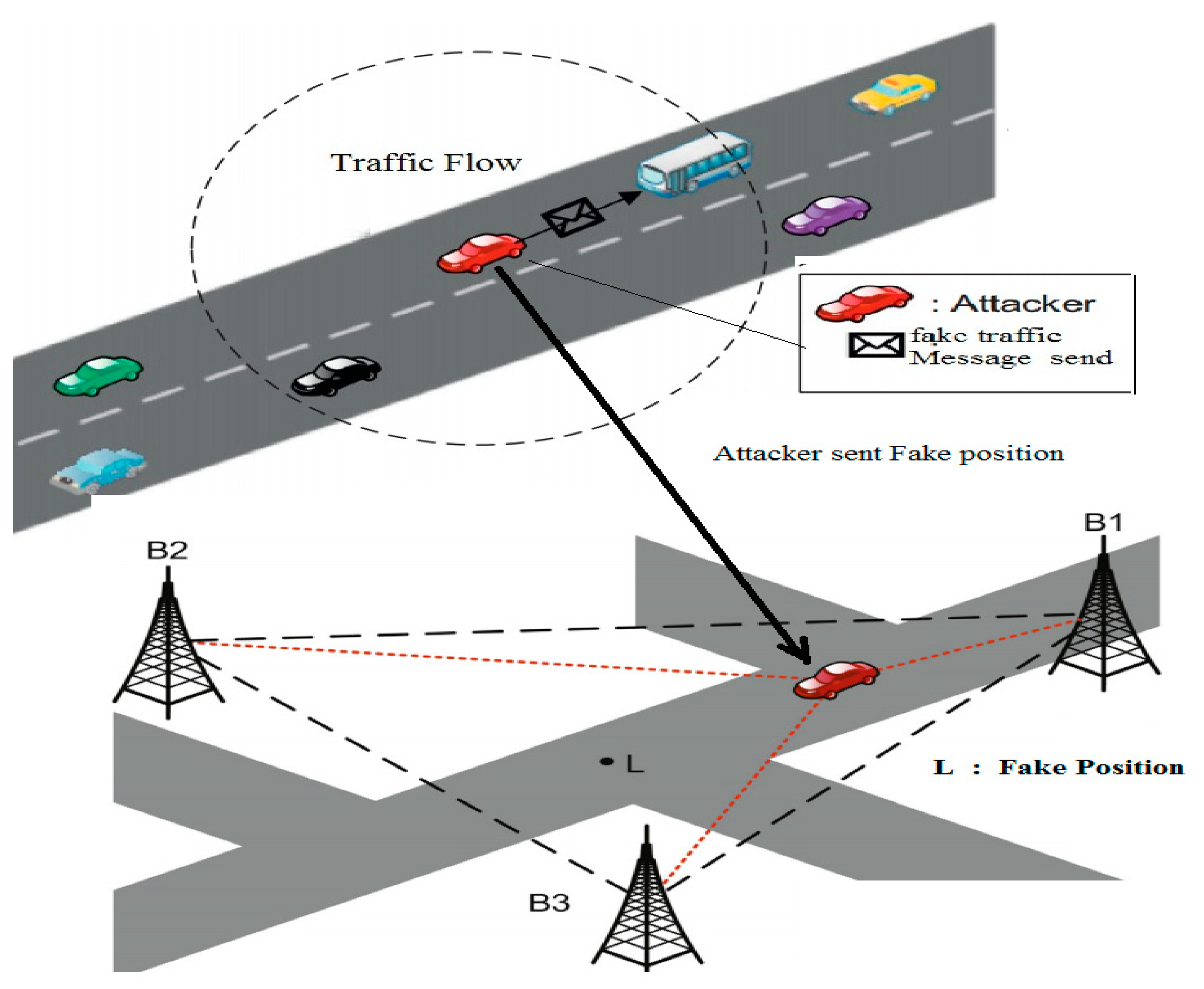
  • Because VANET is a highly dynamic network and the attacked time will be very short, the receiving information of the vehicle must be verified and responded quickly. In other words, the veracity and reliability of vehicle messages must be able to be determined quickly and accurately in VANET [16].
  • Although IDS is a reliable way to protect VANET, it is difficult to solve extra inspection time and loads with the increasing number of vehicles.
A number of studies have been conducted in the IDS area of VANET. A framework that combines creditworthiness scores with rule-based detection is used for IDS in VANET [15,17]. However, there is a particularly serious disadvantage of false alarms, detection times and load problems when the number of vehicles increases. A statistical-based approach was used for IDS [18]. Several studies established on the proposition of a system to detect attacks on vehicles based on matching IDS [19,20,21]. Although it has high detection accuracy and efficiency, it can only detect attacks that match their rules and ignore other unknown attacks. However, when using these types of methods, the distribution of the detected data must be known in advance, which is often difficult. In [22], a new mechanism is provided in IDS that uses Bayesian theory to switch IDS status (active or idle) to reduce overhead and detection time. Unfortunately, it is difficult to detect attacks that occur during the IDS’s idle state, which can compromise the accuracy of IDS detection.

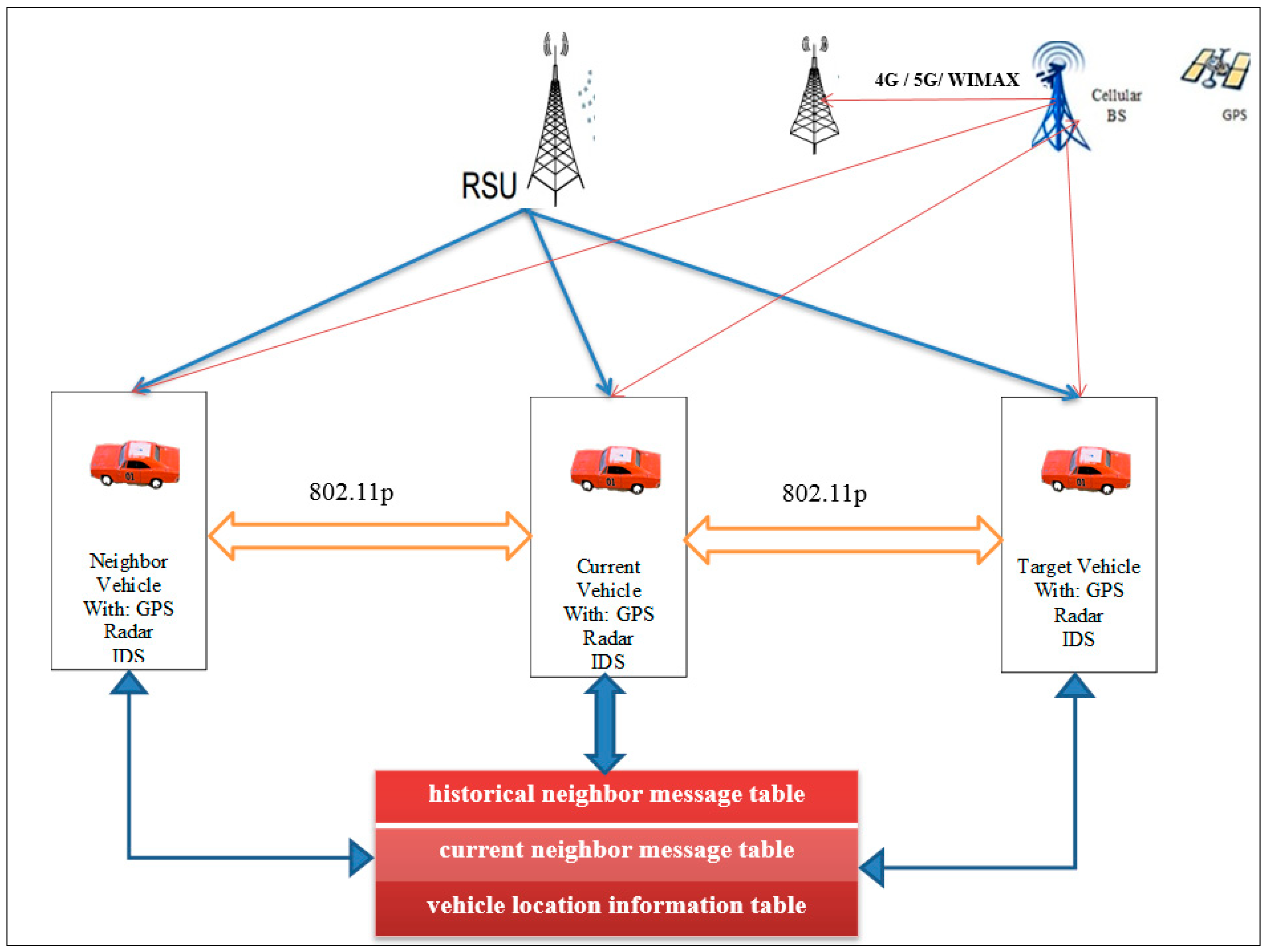
2. Vehicle Ad Hoc Network (VANET) Model

A generic VANET structure can be obtained according to the previous VANET [22,23,24], as shown in Figure 1. In this VANET structure, each vehicle will be installed several devices, such as: GPS, Radar, IDS and so on. Among them, GPS can get the current position of the vehicle. Radar is used to measure the communication signals among vehicles. IDS are used to detect attacks from inside and outside the vehicle. By sending a message, the vehicle can communicate with each other vehicles within its communication domain. At the moment of vehicle communication, vehicles can be divided into three different roles (current vehicle, neighbor vehicle and target vehicle). The current vehicle is defined for each vehicle itself, and the neighbor vehicle is the vehicle in the communication domain of the current vehicle, and the target vehicle is a special neighbor vehicle whose message is being processed by the current vehicle. In addition, each vehicle contains three data tables, namely: the historical neighbor message table, the current neighbor message table and the vehicle location information table. The data in these tables will be used in driving decisions to enhance the driving experience.

2.1. VANET Model. Measurements

On a freeway, the vehicle can calculate the density of vehicles by counting the number of different vehicles in the historical neighbor’s message table. In addition, each vehicle gets location coordinates (Xposown and Yposown) by GPS. It is important to note that the vehicle does not have direct access to the flow of traffic ( Flowown ¯ ) and the distance between two vehicles (Do&n). The Flowown ¯ needs to be calculated from the model of Greenshield [25], and (Do&n) can be calculated from the free space model [26].
The Greenshield model is considered as a fairly accurate model for describing the relationships among speed (v) (Km/hr), density (k) (veh/Km) and traffic flow (q) [25]. The parameter vf can be defined as the free mean speed at which the vehicle density is zero. With the density increasing, the speed will decrease, until the maximum kj (congestion density) (veh/Km) is achieved. This is the case of vehicle congestion. The relationship between speed and density is expressed as follows:
v = v f v f k j k
The traffic flow is represented as:
q = k × v
Hence,
q = ( v f v f k j k ) k
The Greenshield model shows that the relationship between traffic flow and the density is parabolic curve. When flow is very low, speed is higher. The drivers are able to travel at a desired speed. As the flow increases, speed gradually decreases. The highest flow shows the transition of noncongested to congested condition. Greenshield’s model shows the relationship between speed and density as follows:
q m = v m k m
where km and vm parameters can be defined by the optimal vehicle density and the optimal speed value, respectively. In this point, the vehicle flow achieves the maximum qm allowed.
MaxSpeed and MaxDensity can be defined by free flow speed and congestion density, respectively in Equations (5) and (6):
S p e e d o w n ¯ = M a x S p e e d D e n s i t y o w n M a x D e n s i t y M a x S p e e d
F l o w o w n = D e n s i t y o w n × S p e e d o w n ¯
The linking between Equations (3), (5) and (6) can produce the following formulas:
S p e e d o w n ¯ = M a x S p e e d M a x S p e e d M a x D e n s i t y D e n s i t y o w n = v f v f k j k
F l o w o w n = D e n s i t y o w n × S p e e d o w n ¯ = k ( v f v f k j k )
Figure 2 explains the graphical relation between the density, speed, and flow.
The free space model was adopted in order to define Do&n model, where Pr(d) is the transmit power, d which is the distance between sender and receiver. Pt is the transmit signal strength, and τ is the wave length. In this model. At this point, the parameter d is the only variable. If the value of d is determined, then the model can be uniquely identified.
P r   ( d ) = τ P t ( 4 π ) 2 ( d ) 2
Since each vehicle is equipped with radar, when it receives a message from a neighbor’s vehicle, it receives the signal strength of neighbor’s vehicle (RSSleng), the wavelength (WLneg) and transmits power (SPneg). Based on the free space model, the vehicle can calculate Do&n according (10).
D o & n = ( S P n e g × W L n e g 2 ( 4 π ) 2 R S S l n e g ) 1 2

2.2. VANET Message Format

In order to communicate with the neighboring vehicles in the current vehicle’s communication domain, each vehicle broadcasts a beacon message (BeaconMsg) for a fixed time period (BeaconT) in the format shown in (11). Where IDoW is the current vehicle ID.
B e a c o n M s g   ( I D o w n ,   F l o w o w n ¯ ,   X p o s o w n ,   Y p o s o w n )
When the current vehicle needs to get the information of the target vehicle from its neighbor vehicle, it will broadcast request message in the format of request message (IDown, IDtag), where IDtag is the ID of the target vehicle. Once the neighbor’s vehicle receives request message, it will broadcast their location coordinates Xposown, Yposown and their distance from the target vehicle (Dn&t) through ResponseMsg. ResponseMsg format which can be defined by ResponseMsg(IDneg, IDtag, Xposown, Yposown, Dn&t). The duration of this process is called response waiting time (WaitingT).

2.3. VANET Information

In order to store the information in VANET (Table 1), each vehicle has three tables. Those tables are the current neighbor message table, the historical neighbor message table and the location information table respectively. The current neighbor message table and the historical neighbor message table are used to store BeaconMsg from a neighbor’s vehicle. The location information table is used to store ResponseMsg. Each of these three tables has an update cycle, which is the same as for BeaconT. When the update time is up, all the contents in the location information table and the historical neighbor message table are deleted, and the content of the current neighbor message table is transferred to the historical neighbor message table.

3. Intrusion Detection System Based on HGNG Neural Network

The IDS can be used to detect VANET attacks, and then take appropriate countermeasures to prevent and reduce the conducted risks. However, when IDS are introduced to VANET some challenges should be overcome:
  • In wired networks, the VANET of IDS cannot be used due to the wireless and mobile features and their dynamic topology features.
  • Because VANET is a highly dynamic network and the attacked time of vehicles will be very short, the receiving information of vehicles should be quickly verified and responded. In other words, the veracity and reliability of vehicle messages in a VANET should be determined quickly and accurately.
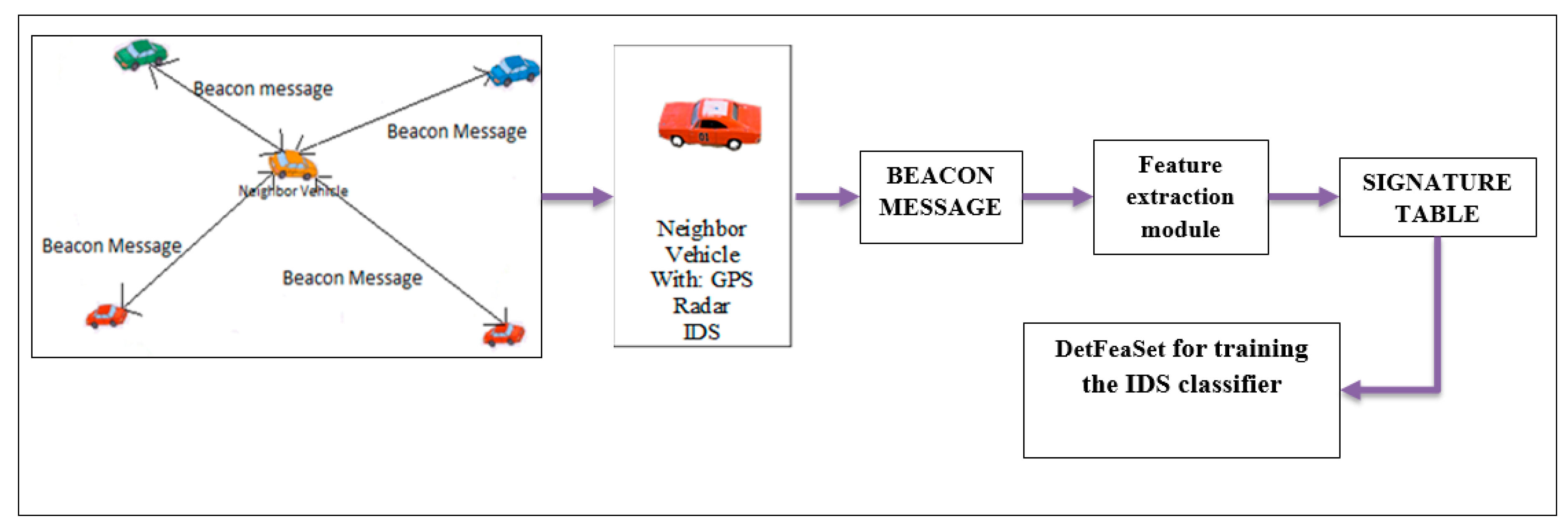
In order to solve the above problems, the new architecture of IDS based on VANET. Model is proposed, which includes the training model without attack and the prediction model with attacks. Then, the two main modules of IDS, namely the feature extraction module and the classifier module, are described in detail. Unlike preprocessing mechanisms in IDS used in wired networks (preprocessing mechanisms only normalization and feature selection for known databases), the feature extraction module is used to quickly convert the measured values of messages from neighboring vehicles to those that can reflect characteristics of vehicle safety features. The classifier module uses clustering neural network algorithm (HGNG) to quickly and accurately detect anomalies in VANET messages.

3.1. HGNG-Based IDS

In order to train the IDS presented in this paper, the training process needs to be performed in a nonattack vehicle situation (under normal conditions), so that the IDS can detect the biased VANET message according to the normal model (as shown in Figure 3).
In VANET, each vehicle calculates measurements, including average traffic and location information, into BeaconMsg and sends it to the neighboring vehicles. In addition, each vehicle receives BeaconMsg from its neighbor’s vehicle within its communications domain. Therefore, the IDS training process is as follows:
First, the vehicle in the VANET extracts the measured value of the BeaconMsg received from the neighboring vehicle through the feature extraction module to form the feature vector. If the vehicle needs the information of the neighbor’s vehicle to assist in extracting the vector of the detected feature, it broadcasts request message and collects the ResponseMsg from the neighbor’s vehicle in WaitingT. Then, the vehicle sends a vector of detection features to the signature table. Finally, when enough detection feature vectors are collected in the trace file of the feature recording module, a DetFeaSet is formed for training the IDS classifier. After the IDS have been trained, it will be placed in the attack vehicle attack detection, as shown in Figure 4.
Once the vehicle receives BeaconMsg from the neighbor vehicle, the same eigenvector extraction strategy is performed as normal. After receiving ResponseMsg, the vehicle filters the ResponseMsg from its neighbor’s vehicle through the filtering mechanism of the feature extraction module. The vehicle then sends the detected feature vector to the classifier to check if there is an attack in the BeaconMsg. Finally, if the classifier determines that there is no deviation of the feature vector, the feature vector is accepted, and the feature is added to the neighbor information table. Otherwise, the feature vector is rejected. If the feature vector is rejected, the neighbor vehicle is highlighted as an attacker vehicle and its ID is put in a blacklist.

3.2. Preprocessing Feature Extraction

As shown in Figure 5, the algorithm has two main parts. One part is the calculation of traffic flow characteristics FlowR. It is based on the principle that the traffic volume of each vehicle should be very similar to the traffic volume of its neighboring vehicles under the same traffic conditions. If an attacking vehicle wants to create a nonexistent incident by sending its reduced fake traffic to other vehicles, its FlowR will be different from normal. Therefore, false information attacks can be detected by FlowR. The other part is to calculate the vehicle position feature, PositionR. PositionR is the deviation between the position coordinate of the neighboring vehicle declaration and the measurement position. When a neighboring vehicle sends a fake location message, it is declaring the location coordinates will go beyond the normal deviation range. Therefore, with PositonR, not only can false message attacks be detected, but also what attacks as well.
Although vehicle location can be verified by any VANET observation model such as accepted signal strength (RSS), and time of arrival. Taking into account the relatively easy access to RSS, this program uses RSS measurement. In the semicooperative detection method, the vehicle position feature can be calculated by either of the following two cases.
If IDtag does not exist in the historical neighbor table (cooperation case), each vehicle first broadcasts request message to its neighbor’s vehicle. When its neighbor’s vehicle receives the RequestMsg, they will broadcast ResponseMsg if they did not receive the IDtag for the RequestMsg in WaitingT. When the time reaches WaitingT, the current vehicle populates ResponseMsg of each neighboring vehicle in its position information table. Then, each vehicle calculates Biaso & t and Biaso & t. The former is the position deviation between itself and the target vehicle, as shown in formula (12). The latter is the deviation between the neighbor’s vehicle and the target vehicle, as shown in Equation (13) (there may be more than one BiaSn & t). Next, each vehicle checks |Biaso & t − BiaSn & t < MaxGap| for ResponseMsg from the attacker vehicle, where MaxGap was determined during training, which is the largest difference between Biaso & t and BiaSn & t.
B i a s o & t = | D o & t ( X p o s o w n X p o s t a g ) 2 + ( Y p o s o w n Y p o s t a g ) 2 |
B i a s n & t = | D n & t ( X p o s n e g X p o s t a g ) 2 + ( Y p o s n e g Y p o s t a g ) 2 |
Finally, if Bias ≥ 3, PositionR is obtained from Equation (14). Otherwise, the characteristic PositionR can not be obtained.
PositionR = 1 n ( B i a s o & t + B i a s n & t )
If there is an IDtag (noncooperation) in the neighbor table, the PositionR of the current vehicle can be directly obtained without the help of a neighbor’s vehicle as shown in Equation (19). This means that the current vehicle does not need to send RequestMsg and wait for ResponseMsg. In Equation (19), B i a s t   t is the position deviation between the current target vehicle and its previous moment, which can be obtained from Equation (16). B i a s o & t is the position deviation between itself and the previous phase of the current target vehicle, as can be seen from Equation (18). Which shows a method of calculating the distance ( D t & t ) between the historical position of the target vehicle and the current position of the target vehicle and the distance ( D o *& t ) between the current position of the current vehicle and the current position of the target vehicle. Because IDtags exist in the historical neighbor table, each vehicle has both historical and current information of its own vehicle and the target vehicle. Therefore, D t & t can be obtained from Equation (15), where ( D t & t is closest to the value of D o & o ). D o   & t can be obtained from Equation (17) according whether D t & t and D o & o already obtained.
D t & t = ( M a x S p e e d 2 ± M a x S p e e d 2 M a x S p e e d 2 A v g F l o w t a g       ) × B e a c o n t      
B i a s t & t = | D t & t ( X p o s t a g X p o s t a g ) 2 + ( Y p o s t a g Y p o s t a g ) 2 |
D o & t = D o & t 2 + D o & o 2 2 D o & t D o & o c o s < T O O
B i a s o & t = | D o & t ( X p o s o w n X p o s t a g ) 2 + ( Y p o s o w n Y p o s t a g ) 2 |
P o s i t i o n R = B i a s o & t +   B i a s t & t   +   B i a s o & t 3

3.3. Based on HGNG Neural Network Outlier Detection

Due to the need for a classifier that can detect attacks in VANET quickly and accurately, HGNG, a neural network with high detection accuracy and low computational complexity, is a good choice. In addition, the paper also presents an improved HGNG on HGNG that enables it to detect abnormalities in IDS more accurately.
The growth-type neural gas (GNG) algorithm, proposed by Fritzke [27], is an extension of the traditional SOM network and Neural Gas algorithm. GNG overcomes the limitations of standard self-organizing map neural networks. The algorithm combines the growth mechanism of GCS neural network with the competitive Hebbian learning rule [28,29]. Moreover, this model does not have the dynamic structure of fixed dimension and adaptively learns the dimension of input sample and the input data in the process of training density. In VANET applications, the GNG network can automatically extract the feature vector PositionR (D(FlowR, PositionR)) and hence the data because there is no topological relationship displayed between Vehicles.
GNG is a dynamic growth self-organizing network based on competitive connection mechanism. It consists of a set of node units A = {c1, c2,…, ck} and the connection C = {(i,j)} between units, i   a n d   j A , (i, j) = (j, i). For each cell, save its two properties: the cell reference vector. ω c R n and accumulation error ϵ c R . For the VANET problem, since the two-dimensional planar contour needs to be constructed, the dimension of the reference vector is 2, which is equal to the dimension of the two components of the input sample point [X, Y]. The mechanism of accumulating errors is introduced to determine where to insert new cells in the network learning process so that the network can grow dynamically. Each pair of links (i, j) has an age attribute of age (i, j), which is used to dynamically delete invalid connections during the learning process. The set of elements connected to a particular cell is N c = { i | i A , ( c , i )   C } constitute its topology neighborhood. The initial GNG network contains a small number of cells and empty connections, as the network learning, and gradually increase the number of units and change the connection, in order to achieve input space topology and spatial geometric approximation.
Taking the feature vector D(FlowR, PositionR) as input sample, the learning process of GNG network is as follows:
  • Initialization A consists of two elements A = {c1, c2, c3}. The coordinates of three randomly selected points in the input sample D(FlowR, PositionR) are used as the reference vectors of c1, c2 and c3. Initialization Unit Connection Set C = {(c1, c2), (c2, c3), (c1, c3)}. Set the current learning step = 0.
  • Learning times, step = step + 1, select a point ε randomly from the input eigenvector as the input sample and find the nearest-neighbor and next-nearest neighbor units of ε in A:
    n 1 = a r g   m i n n A ε ω n
    n 2 = a r g   m i n n A \ n 1   ε ω n
    where · represents the norm of the Euclidean space vector.
  • If there is no connection between n1 and n2, add the connection between the two cells:
    C = C { ( n 1 , n 2 ) } .   i f   ( n 1 , n 2 ) ¯ C
    Set age (n1, n2) = 0 for connection (n1, n2). And increase the age of all connections for cell n1:
    { n 1 , } = { ( n 1 , i ) | i N n 1 }
    a g e ( n 1 , i ) = a g e ( n 1 , i ) + 1 ,   ( n 1 , i ) ( n 1 , )
  • Update the error of n1 by the square of the Euclidean distance between σ and the reference vector of the nearest neighbor cell n1:
    ε n 1 = σ ω n 1 2
  • Update the reference vectors of n1 and its topological neighbors with the following rules:
    ω n 1 = γ b ( σ ω n 1 )
    ω i = γ n ( σ ω i ) ,   i N n 1
    where γb and γn represent the learning rate of winning unit n1 and its topology neighborhood, respectively.
  • If the learning frequency is an integral multiple of the unit insertion frequency φ, insert the new unit as follows:
    Find the unit p with the largest accumulation error and the maximum error unit in the topology neighborhood of p q
    p = a r g   m a x i A ε i
    q = a r g   m a x i N p ε i
    Add a new node element K whose reference vector and error are the mean of p and q:
    A = A { k } ω k = ω p + ω q 2   a n d   ε k = ε p + ε q 2
    Delete the connection (p, q), add new connections (p, k) and (q, k) and reduce the accumulation error of units p, q, k by a percentage:
    C = C / ( p , q ) { ( p , k ) , ( q , k ) }
    ε i = α ε i ,   i ( p , q , k )
  • Reduce the cumulative error of all units by a fixed percentage ε i = β ε i , i A .
  • Delete all { n 1 , } all connections whose age is greater than the parameter αmax, and delete if the number of connections to a cell is 0 at the time of deletion:
    C = C { ( { n 1 , i ) | a g e ( n 1 , j ) α m a x , i N n 1 }
    C = C / { j   |   N j = , j A   }
  • If the set termination condition is reached, for example, the number of learning step > stepmax, then terminate; otherwise, skip to step (ii) to continue learning.
The essence of GNG algorithm is to transform the network in the neuron’s reference vector space by the competitive Hebbian learning rules so that the network composed of neurons gradually converge to the geometric distribution and topological structure of the input sample space in a probabilistic manner. The transformation includes two types: Geometric transformations and topological transformations Geometrical transformations are simpler, and the local neuron reference vectors are moved by Step (v) to continuously change the receptive field of neurons in the signal space and converge them into a local cluster center. Clustering forms the sample space A vector quantization, in order to reduce the quantization error, need to insert a new cluster center by Step 6 to assign a local error, and Step (ix) to delete the cluster center which contributes little to the error reduction. Meanwhile, the topology transformation in the learning process is performed by Step (iii), Step (iv), Step (viii). The specific method is to insert and delete inter-neuronal connections, detect the wrong connections that should be deleted through neuronal age-aging and update mechanisms, and if a connection has a high response frequency under the influence of the input signal Retain, delete if inactive for a long time.
In the process of GNG learning, the coordination between geometric transformation and topological transformation should be kept in place [30]. The change of neuron position may lead to the failure of topological connection. If the two parameters γb and γn are set too large, will be larger, and the topology transformation too late to delete the resulting error connection. Which will lead to grid self-intersection and a large number of wrong connections. GNG algorithm Step 6, the new neurons inserted at a fixed frequency may produce outdated nerves. If the number of neurons grows too fast, not only does it increase the burden of finding the winning neuron, but also the topology transformation cannot establish an effective connection near the new cell, resulting in a large number of holes in the network. In addition, Step 8 is deleted by a fixed age threshold. However, the age-based deletion mechanism does not guarantee the constraint (1) and constraint (2) of the triangular mesh reconstruction problem. If the edge of the deletion is not invalid edge, it will produce holes in the triangle mesh; and if the follow-up learning process repeatedly inserts and delete the edge, this will lead to the structural instability of the neural network and cannot converge. Based on the above analysis, it is necessary to improve the neuronal insertion and deletion mechanism of the GNG algorithm for the constraint of the triangular mesh reconstruction.
Because the outline of hierarchical data is composed of one ring, the node on the ring can only be connected with two nodes, that is, the predecessor and successor of the node. However, with GNG algorithm, it is easy to form a node connection because there is no limit of number of nodes connected More than two bifurcated structures or insufficient node connections lead to ring breakage. In order to limit the scope of the solution space, a constraint mechanism needs to be introduced in the GNG so that the GNG network will try its best to satisfy the constraint of only two immediate topological neighbors.
In the GNG algorithm, step (iii) is modified as:
If there is no connection between n1 and n2, first add the connection between the two cells:
C = C { ( n 1 , n 2 ) }   if   ( n 1 , n 2 ) ¯ C
Set age (n1, n2) = 0 for connection (n1, n2). And increase the age of all connections for cell n1:
{ n 1 , } = { ( n 1 , i ) | i N n 1 }
a g e ( n 1 , i ) = a g e ( n 1 , i ) + 1   ( n 1 , i ) { n 1 , }  
At this point, if the number of connections for a cell is greater than 2, a bifurcated structure is formed, removing the oldest connections from { n 1 , } and { n 2 , } . When a new connection is inserted, the oldest connections are detected and deleted, ensuring that each node unit is directly connected to the two surrounding units.
In the process of hierarchical contour reconstruction of point cloud data by GNG algorithm, the data involved in the outline of each layer take values within the range of δ near the layering plane. In order to ensure the accuracy of the reconstructed contour, a weighting mechanism is introduced into the learning rule. During the neural network learning, the points far away from the plane of stratification have less influence on the neurons, while point cloud from the plane is more affected, so step (v) is modified as:
Update the reference vectors of n1 and its topological neighbors with the following rules:
ω n 1 = γ b ( σ ω n 1 ) F ( | σ z P o s | )
ω i = γ n ( σ ω i ) F ( | σ z P o s | ) ,   i N n 1
where δz represents the (x, y) coordinates of the sample point, and F(x) is a weight function inversely proportional to x, indicating that the farther the point is from the layered plane, the smaller the contribution to the unit weight vector. In the actual calculation of the total weight function take Gaussian function:
F ( x ) = e x 2 / e ( t ) 2
Among them, the center of Gaussian function is 0, c(t) is Gaussian radius, decay with time. It can be seen from the equation that the farther away from the layering plane, the smaller the weight adjustment range, so as to ensure that the network finally converges to a stable state. In addition, when using GNG network to reconstruct the outline data of each layer, if each layer initializes three neurons by adopting the initial step of GNG, each layer needs to be rebuilt from the initial GNG network during the reconstruction and finally reconstructed the complete outline of the data. In this paper, based on the principle of geometric continuity of solid parts, that is, the principle that the contour of adjacent layers of solid parts does not change much, the GNG network structure studied in the previous layer contour reconstruction is taken as the initial structure of the next layer. When the change is small, the learning process converges quickly. When the topology of the interlayer ring structure changes suddenly, the topological structure can be automatically changed during the GNG learning process.
HGNG, defined as a tree of graphs, is a clustering neural network that overcomes the original space constraints of GNG [31]. It has a hierarchical, nonfixed structure [32]. It consists of multiple layers, consisting of several independent GNGs, the number and size of which are determined during the training phase. The procedure to learn such hierarchy is detailed in the following. The process starts by training the root graph with the overall set of training samples. Each time that a graph must be trained with training set S, this is done according to the algorithm specified in Section 2. If the resulting number of units is H = 2, then the graph is pruned, because it is too small to represent any important features of the input distribution. Otherwise, a new graph is created for each unit i and the training process is invoked recursively with the receptive field of unit i as the training set:
V i = { ε V | i = a r g   m i n i A ε ω i }
This recursive process continues until a prespecified number of levels are reached. The elimination of the graphs is with fewer than three units and the split of the training set together in order to attain a parsimonious hierarchy, i.e., one with a reduced number of graphs and units. This is because lower graphs in the tree cannot have many units because their training sets are smaller. It is worth noting that many of the created graphs will eventually be pruned right after their training, so that the fact that a graph is created for each unit does not lead to uncontrolled growth.

4. Performance Evaluations

4.1. Experimental Environment

Simulation experiments are based on NS [33], and urban traffic simulation tools (SUMO) [34]. NS2 provides a relatively complete low-level protocol and a simple programming interface. SUMO is a software tool used to generate vehicle traffic by specifying the speed, type, behavior, and number of vehicles. SUMO can also set the road type and conditions. While simulating the IDS in this article, SUMO is used to generate the move trace file, and NS2 is used to load these trace files and run the IDS.

4.2. Experimental Parameters

In the experimental simulation, the experimental parameters are shown in Table 2. The vehicle can run on a 5-km-long highway with two lanes and can communicate with other vehicles within 500 m of the transmission range according to the communication protocol 802.11p. To avoid generating too much data in a simulation, we set the simulation time to 165 s, the vehicle arrival interval to 1 s and the transmission interval (BeaconT) to 0.5. In order to ensure that ResponseMsg has enough time to arrive, this article sets the response latency (WaitingT) to 0.2 s. Taul and Taut (HGNG-related two parameters) were set to 0.1 and 0. 01.

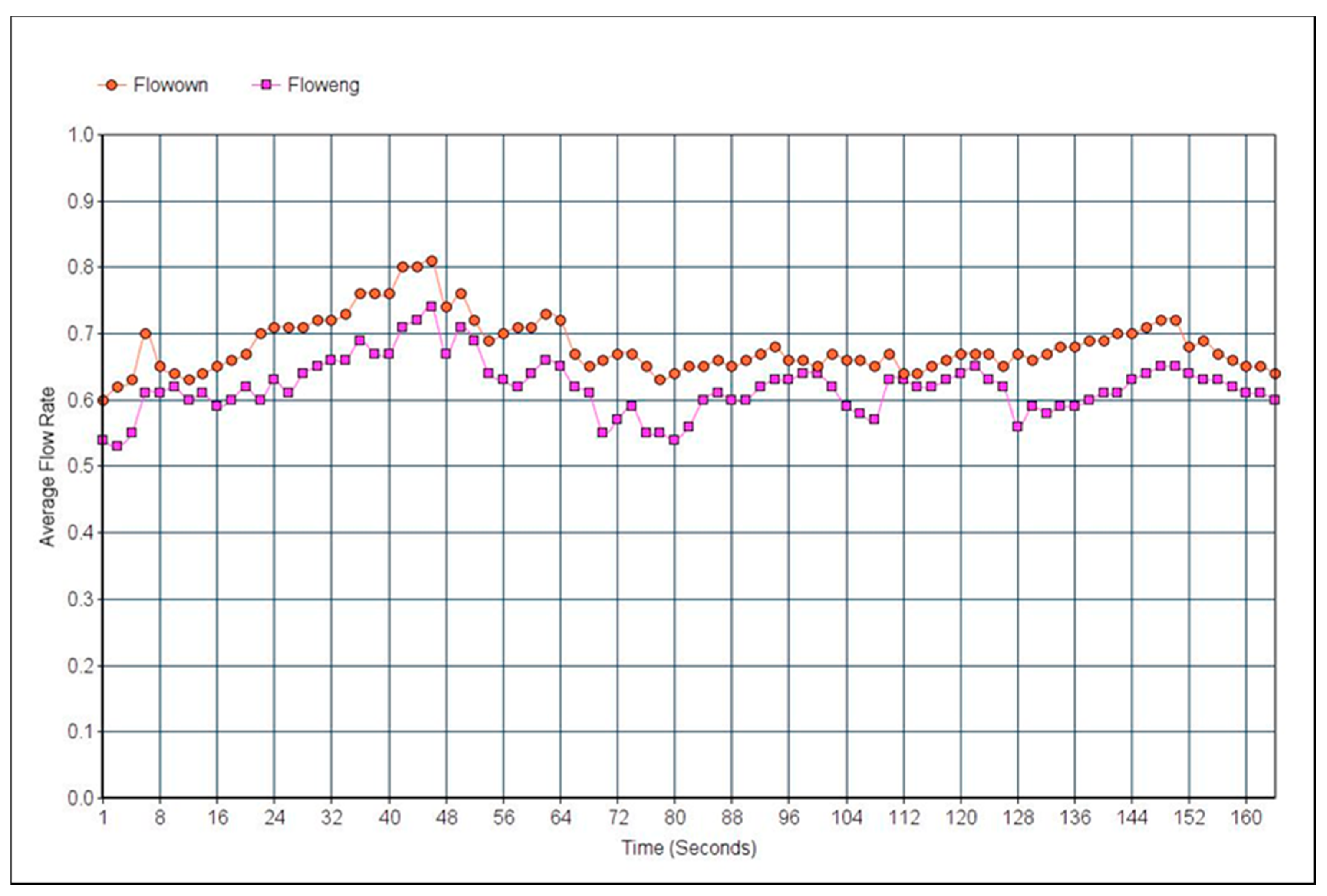
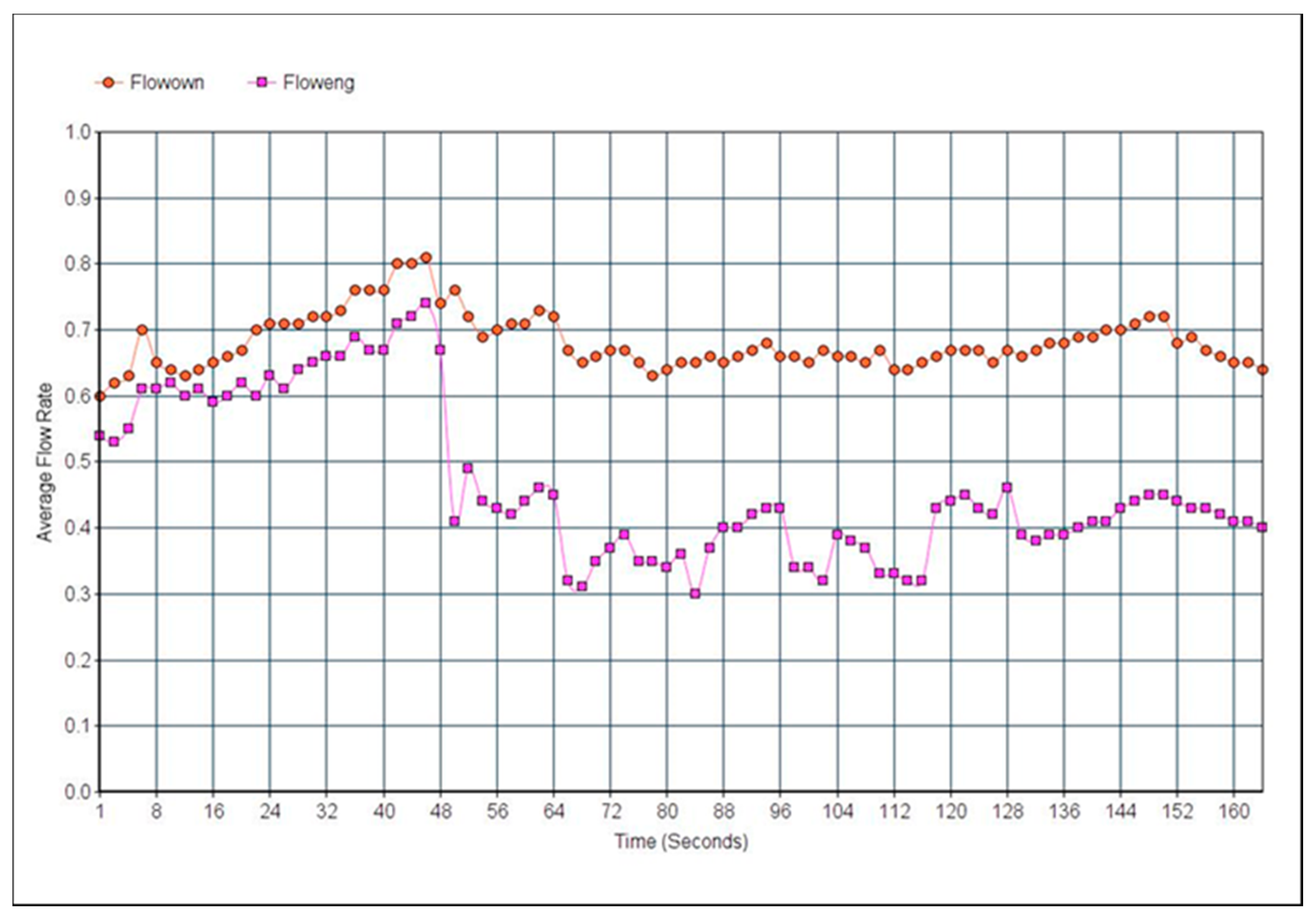
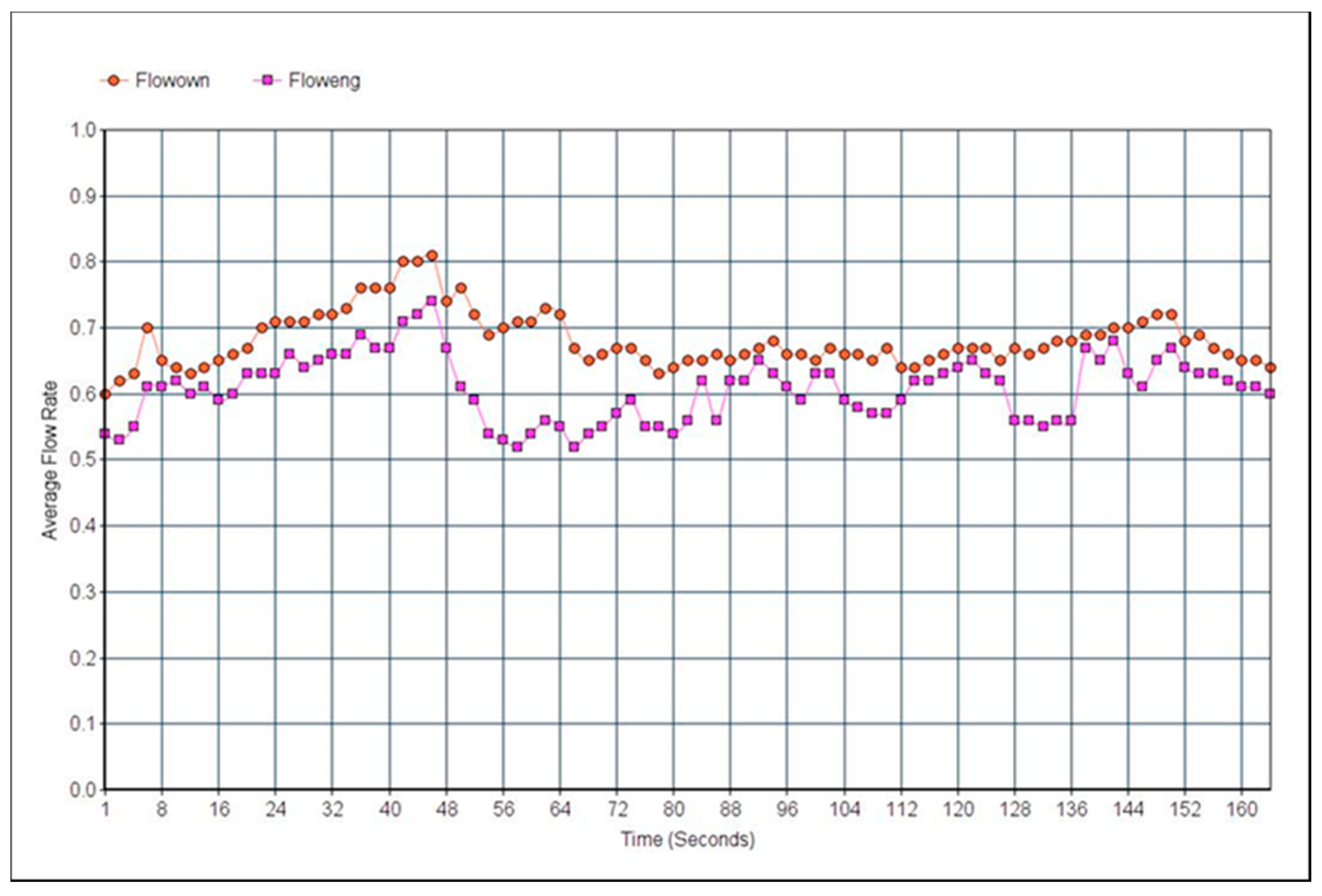
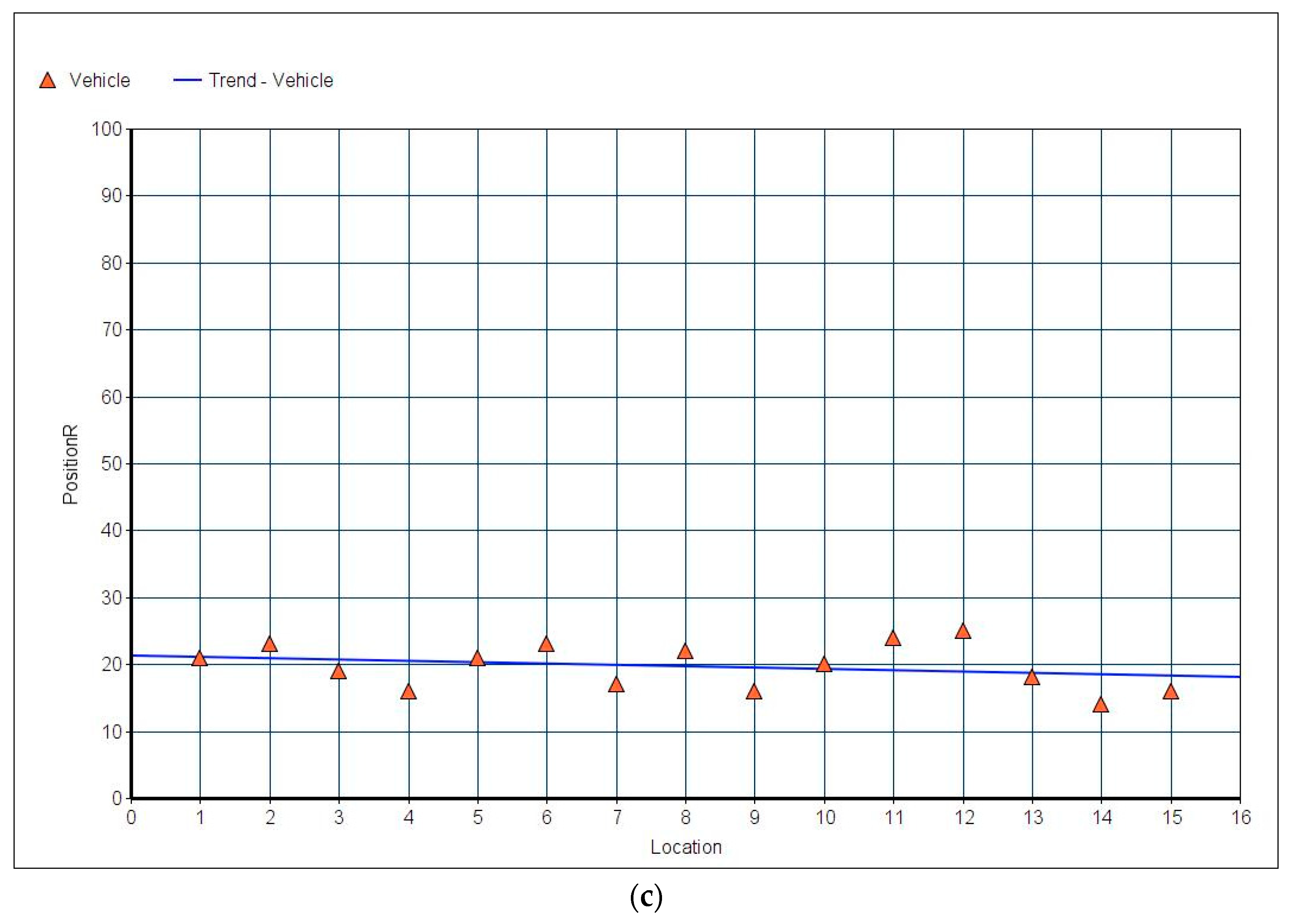
4.3. Experimental Results

In order to collect data to detect attacks, this experiment uses different simulation scenarios. In this experiment we collect data in the absence of a vehicle attack (normal conditions) to train IDS. In addition, IDS is tested in the presence of an attacking vehicle (unusual situation) to understand the IDS work in this article. In the following, this experiment verifies the validity of this system IDS in two aspects (traffic flow detection and vehicle location detection).
In order to verify the validity of IDS proposed in this paper, the experiment collect the average flow rate ( Flowown ¯ ) of vehicles randomly selected under different conditions and the flow of its reception ( Floweng ¯ ), as shown in Figure 6, Figure 7 and Figure 8. Figure 7 shows the data under normal conditions. It can be observed ( Flowown ¯ and ( Floweng ¯ ) values are fairly close with very slight variation. Then, 50% of the vehicles attacked are inserted and they send a fake traffic flow (close to the blue dot at the bottom of the Figure 7 and Figure 8) after t = 50 s. In the absence of IDS (Figure 7), ( Floweng ¯ ) decreases with acceptance of all messages (including normal and abnormal messages) and decreases from the legitimate vehicle ( Floweng ¯ ) (the blue dot near the red curve) as it also Affected vehicles. In the case of IDS, as shown in Figure 8, it can be observed that the IDS proposed in this paper can detect Flowneg and then reject the abnormal message, so that the ( Flowown ) ¯ value is similar to normal. This means that the IDS proposed in this paper is effective in traffic flow detection.
In verifying the validity of the IDS proposed in this paper for vehicle position detection, the experiment collects the PositionR values of vehicles randomly selected in different situations and displayed in Figure 9. First run the simulation under normal conditions. Figure 9a presents the values of the PositionR at a relatively low level. The coordinates of the PositionR here are caused by some unavoidable errors, for example device errors, transmission errors, and so on. Hence, a noticeable variation was attained. On the other hand, assuming that there is 50 percentage of attack vehicles in an abnormal situation, the attacking vehicle changes their position information in BeaconMsg and ResponseMsg, as exhibited in Figure 9b,c. In the absence of IDS (Figure 9b), many PositionR values appear to deviate significantly from normal at this point. Finally, IDS in each vehicle is activated (Figure 9c), it can be notice here almost all PositionR values are close to normal, which indicates the efficiency of the adopted IDS in the vehicle position detection. Therfore and based on those two-step verification mechanism, it is approved the feasibility of the applied modeling strategy.

5. Conclusions

In the current research, a new modeling strategy is proposed called HGNG-based IDS to detect possible attacks in the VANET. The IDS mainly contains a new feature extraction mechanism and classifier based on a HGNG neural network. The proposed feature extraction mechanism is used to extract two main features: traffic flow features and vehicle position features. To extract the location features more effectively, it adopted a semicooperative procedure to extract the location features in the feature extraction mechanism. It not only collects the location feature by cooperatively collecting the current location information of the neighboring vehicles, it also can extract the location features according to the historical location information. Further, in the HGNG-based classifier, a two-step verification mechanism was used for more accurate judgment of vehicle message anomalies. In addition, we conducted an experiment where the proposed IDS was evaluated and observed. The findings of the current study evidenced the capacity of the proposed modeling strategy to the other IDS in terms of accuracy, stability, processing efficiency, and message size.

Author Contributions

Formal Analysis, G.S. and G.A.; Methodology, A.A.A.; Writing–Original Draft Preparation, G.A.

Funding

This research received no external funding.

Conflicts of Interest

The authors declare no conflict of interest.

References

  1. Al-Sultan, S.; Al-Doori, M.M.; Al-Bayatti, A.H.; Zedan, H. A comprehensive survey on vehicular Ad Hoc network. J. Netw. Comput. Appl. 2014, 37, 380–392. [Google Scholar] [CrossRef]
  2. Sarika, S.; Pravin, A.; Vijayakumar, A.; Selvamani, K. Security Issues in Mobile Ad Hoc Networks. Procedia Comput. Sci. 2016, 92, 329–335. [Google Scholar] [CrossRef]
  3. Lee, K.C. Geographic Routing in Vehicular Ad Hoc Networks. Ph.D. Thesis, University of California at Los Angeles, Los Angeles, CA, USA, 2010. [Google Scholar]
  4. Jiang, D.; Delgrossi, L. IEEE 802.11p: Towards an international standard for wireless access in vehicular environments. In Proceedings of the VTC Spring 2008—IEEE Vehicular Technology Conference, Singapore, 11–14 May 2008. [Google Scholar]
  5. Leontiadis, I.; Marfia, G.; Mack, D.; Pau, G.; Mascolo, C.; Gerla, M. On the Effectiveness of an Opportunistic Traffic Management System for Vehicular Networks. IEEE Trans. Intell. Transp. Syst. 2011, 12, 1537–1548. [Google Scholar] [CrossRef] [Green Version]
  6. Alasmary, W.; Zhuang, W. Mobility impact in IEEE 802.11p infrastructureless vehicular networks. Ad Hoc Netw. 2012, 10, 222–230. [Google Scholar] [CrossRef] [Green Version]
  7. McGibney, J.; Botvich, D.; Balasubramaniam, S. A combined biologically and socially inspired approach to mitigating ad hoc network threats. In Proceedings of the 2007 IEEE 66th Vehicular Technology Conference, Baltimore, MD, USA, 30 September–3 October 2007. [Google Scholar]
  8. Raya, M.; Papadimitratos, P.; Gligor, V.D.; Hubaux, J.P. On data-centric trust establishment in ephemeral ad hoc networks. In Proceedings of the 27th Conference on Computer Communications, Phoenix, AZ, USA, 13–18 April 2008. [Google Scholar]
  9. Wex, P.; Breuer, J.; Held, A.; Leinm, T. Trust Issues for Vehicular Ad Hoc Networks. In Proceedings of the VTC Spring 2008—IEEE Vehicular Technology Conference, Singapore, 11–14 May 2008. [Google Scholar]
  10. Lu, R.; Lin, X.; Luan, T.H.; Liang, X.; Member, S.; Shen, X.S. Pseudonym Changing at Social Spots: An Effective Strategy for Location Privacy in VANETs. IEEE Trans. Veh. Technol. 2012, 61, 86–96. [Google Scholar] [Green Version]
  11. Minhas, U.F.; Zhang, J. Towards Expanded Trust Management for Agents in Vehicular Ad-hoc Networks. Int. J. Comput. Intell. Appl. Theory Pract. 2016, 2, 1–13. [Google Scholar]
  12. Kargl, F.; Papadimitratos, P.; Buttyan, L.; Müter, M.; Schoch, E.; Wiedersheim, B.; Thong, T.V.; Calandriello, G.; Held, A.; Kung, A.; et al. Secure vehicular communication systems: Implementation, performance, and research challenges. IEEE Commun. Mag. 2008, 11, 110–118. [Google Scholar] [CrossRef]
  13. Ruj, S.; Cavenaghi, M.A.; Huang, Z.; Nayak, A.; Stojmenovic, I. On Data-centric Misbehavior Detection in VANETs. In Proceedings of the 2011 IEEE Vehicular Technology Conference (VTC Fall), San Francisco, CA, USA, 5–8 September 2011; pp. 1–5. [Google Scholar]
  14. Raya, M.; Papadimitratos, P.; Aad, I.; Jungels, D.; Hubaux, J.P. Eviction of misbehaving and faulty nodes in vehicular networks. IEEE J. Sel. Areas Commun. 2007, 8, 1557–1568. [Google Scholar] [CrossRef]
  15. Sedjelmaci, H.; Senouci, S.M.; Feham, M. An efficient intrusion detection framework in cluster-based wireless sensor networks. Int. J. Appl. Eng. Res. 2014, 9, 5968–5974. [Google Scholar] [CrossRef]
  16. Parno, B.; Perrig, A. Challenges in securing vehicular networks. Work. Hot Top. Netw. 2015, 2, 1–6. [Google Scholar]
  17. Sedjelmaci, H.; Senouci, S.M. An accurate and efficient collaborative intrusion detection framework to secure vehicular networks. Comput. Electr. Eng. 2015, 43, 33–47. [Google Scholar] [CrossRef]
  18. Yu, B.; Xu, C.Z.; Xiao, B. Detecting Sybil attacks in VANETs. J. Parallel Distrib. Comput. 2013, 73, 746–756. [Google Scholar] [CrossRef]
  19. Sedjelmaci, H.; Senouci, S.M.; Abu-Rgheff, M.A. An efficient and lightweight intrusion detection mechanism for service-oriented vehicular networks. IEEE Intern. Things J. 2014, 1, 570–577. [Google Scholar] [CrossRef]
  20. Mokdad, L.; Ben-Othman, J.; Nguyen, A. DJAVAN: Detecting jamming attacks in Vehicle Ad hoc Networks. Perform. Eval. 2015, 87, 47–59. [Google Scholar] [CrossRef]
  21. Sedjelmaci, H.; Bouali, T.; Senouci, S.M. Detection and prevention from misbehaving intruders in vehicular networks. In Proceedings of the 2014 IEEE Global Communications Conference, Austin, TX, USA, 8–12 December 2014. [Google Scholar]
  22. Sedjelmaci, H.; Senouci, S.M.; Ansari, N. Intrusion Detection and Ejection Framework Against Lethal Attacks in UAV-Aided Networks: A Bayesian Game-Theoretic Methodology. IEEE TRASECTION Syst. 2017, 18, 1143–1153. [Google Scholar] [CrossRef]
  23. Yan, S.; Member, S.; Malaney, R.; Nevat, I.; Peters, G.W. Optimal Information-Theoretic Wireless Location Verification. IEEE Transic. 2014, 63, 3410–3422. [Google Scholar] [CrossRef] [Green Version]
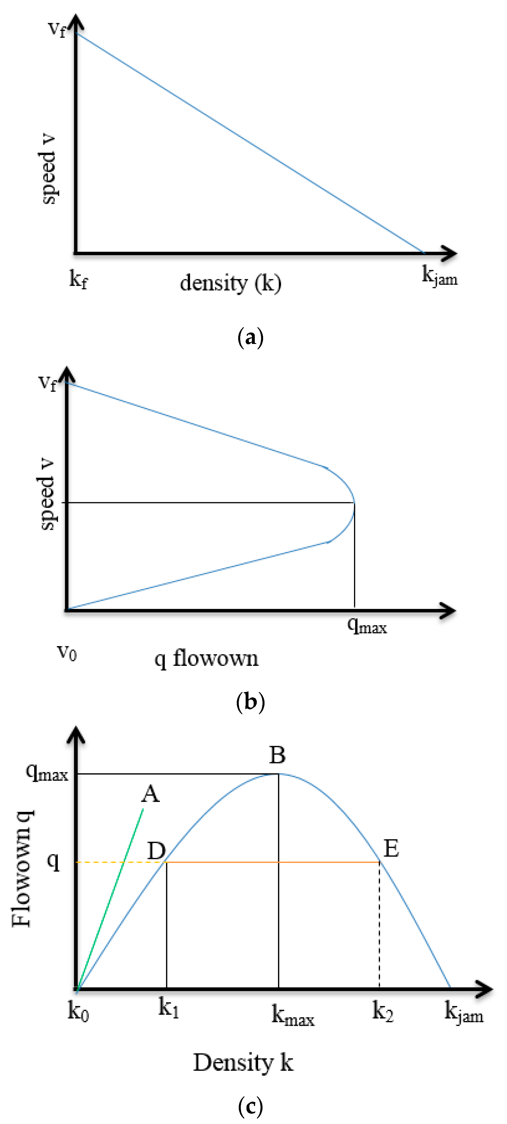
  24. Rakha, H.; Crowther, B. Comparison of Greenshields, Pipes, and Van Aerde vehicle-following and traffic stream models. J. Transp. Res. Board 2002, 1802, 248–262. [Google Scholar] [CrossRef]
  25. Azlan, N.N.N.; Rohani, M.M. Overview of Application of Traffic Simulation Model. In Proceedings of the Malaysian Technical Universities Conference on Engineering and Technology (MUCET 2017), Penang, Malaysia, 6–7 December 2017; pp. 1–6. [Google Scholar]
  26. Sommer, C.; Eckhoff, D.; German, R.D. A computationally inexpensive empirical model of IEEE 802.11 p radio shadowing in urban environments. In Proceedings of the 2011 Eighth International Conference on Wireless On-Demand Network Systems and Services, Bardonecchia, Italy, 26–28 Janurary 2011; pp. 84–90. [Google Scholar]
  27. Fritzke, B. A Growing Neural Gas Network Learns Topologies. In Proceedings of the 7th International Conference on Neural Information Processing Systems, Denver, CO, USA, 28 November–1 December 1994. [Google Scholar]
  28. Saleem, W.; Schall, O.; Patane, G.; Belyaev, A.S.H. On stochastic methods for surface reconstruction. Vis. Comput. 2007, 6, 381–395. [Google Scholar] [CrossRef]
  29. Mari, J.F.; Saito, J.H.; Poli, G.L.A. Improving the neural meshes algorithm for 3D surface reconstruction with edge swap operations. In Proceedings of the 2008 ACM Symposium on Applied Computing (SAC), Fortaleza, Brazil, 16–20 March 2008; pp. 1236–1240. [Google Scholar]
  30. Fritzke, B. A Growing Neural Gas Network Learns Topologies. Adv. Neural Inf. Process. Syst. 1995, 7, 625–632. [Google Scholar]
  31. Satomi, M.; Masuta, H.; Kubota, N. Hierarchical growing neural gas for information structured space. In Proceedings of the 2009 IEEE Workshop on Robotic Intelligence in Informationally Structured Space, Nashville, TN, USA, 30 March–2 April 2009. [Google Scholar]
  32. Rauber, A.; Merkl, D.; Dittenbach, M. The growing hierarchical self-organizing map: Exploratory analysis of high-dimensional data. IEEE Trans. Neural Netw. 2002, 13, 1331–1341. [Google Scholar] [CrossRef] [PubMed]
  33. Issariyakul, T.; Hossain, E. Introduction to Network Simulator NS2, 1st ed.; Springer: Boston, MA, USA, 2012; ISBN 9781461414063. [Google Scholar]
  34. Behrisch, M.; Bieker, L.; Erdmann, J.; Krajzewicz, D. SUMO-Simulation of Urban MObility: An Overview. In Proceedings of the SIMUL 2011: The Third International Conference on Advances in System Simulation, Barcelona, Spain, 23–28 October 2011. [Google Scholar]
Figure 1. Vehicle ad hoc network model.
Jsan 07 00041 g001
Figure 2. (a) Speed vs. density; (b) speed vs. flowown and (c) flowown vs. density.
Jsan 07 00041 g002
Figure 3. Vehicle receives beacon messages from neighbor vehicles.
Jsan 07 00041 g003
Figure 4. Detection attack in VANET.
Jsan 07 00041 g004
Figure 5. Preprocessing feature extraction.
Jsan 07 00041 g005
Figure 6. Average flow (Flowown) and reception flow (Floweng) rates in normal conditions.
Jsan 07 00041 g006
Figure 7. Average flow rate and reception flow time rates with 50% vehicle attacks.
Jsan 07 00041 g007
Figure 8. Average flow rate and reception flow time rates with 50% vehicle attacks (with IDS).
Jsan 07 00041 g008
Figure 9. (a) PositionR of vehicles in normal conditions. (b) PositionR of vehicles in normal conditions with 50% vehicle attacks. (c) PositionR of vehicles in normal conditions with 50%.
Jsan 07 00041 g009aJsan 07 00041 g009b
Table 1. VANET Information Table.
Current Neighbor Message TableStore B e a c o n M s g
Historical Neighbor Message TableStore B e a c o n M s g
Location Information TableStore R e s p o n s e M s g
Table 2. Parameter setting.
ParameterValue
Experimental scene2 lane of 5 km highway
Maximum vehicle speed100 km/h
Wireless communication protocol802.11p
Transmission range500 m
Simulation time165 s
Vehicle arrival interval1 s
Transmission interval0.5 s
The corresponding waiting times0.2 s
Tau1, Tau20.1, 0.01

