Multiscale and Hierarchical Classification for Benthic Habitat Mapping


Centre for Integrative Ecology, School of Life and Environmental Sciences, Deakin University, P.O. Box 423, Warrnambool, VIC 3280, Australia
*
Author to whom correspondence should be addressed.
Geosciences 2018, 8(4), 119; https://doi.org/10.3390/geosciences8040119
Submission received: 28 February 2018
/
Revised: 29 March 2018
/
Accepted: 30 March 2018
/
Published: 2 April 2018
(This article belongs to the Special Issue Marine Geomorphometry)
Abstract
:Developing quantitative and objective approaches to integrate multibeam echosounder (MBES) data with ground observations for predictive modelling is essential for ensuring repeatability and providing confidence measures for benthic habitat mapping. The scale of predictors within predictive models directly influences habitat distribution maps, therefore matching the scale of predictors to the scale of environmental drivers is key to improving model accuracy. This study uses a multi-scalar and hierarchical classification approach to improve the accuracy of benthic habitat maps. We used a 700-km2 region surrounding Cape Otway in Southeast Australia with full MBES data coverage to conduct this study. Additionally, over 180 linear kilometers of towed video data collected in this area were classified using a hierarchical classification approach. Using a machine learning approach, Random Forests, we combined MBES bathymetry, backscatter, towed video and wave exposure to model the distribution of biotic classes at three hierarchical levels. Confusion matrix results indicated that greater numbers of classes within the hierarchy led to lower model accuracy. Broader scale predictors were generally favored across all three hierarchical levels. This study demonstrates the benefits of testing predictor scales across multiple hierarchies for benthic habitat characterization.
1. Introduction
Development of hydrographic survey technologies over the past few decades has provided an ever more focused lens through which scientists can study the relationships between the physical nature of the seafloor and the benthic communities found there. Multibeam echosounders (MBES) provide the ability to collect detailed full-coverage information on fine-scale features that are required for the development of benthic habitat maps [1,2]. However, the spatial scale of drivers of habitat distribution are often mismatched and in many cases there is a need to explore seafloor structure at multiple spatial scales in order to match local drivers of habitat distribution [3]. Understanding resource and habitat distribution is crucial for effective management. As a result, maps that accurately reflect distribution of key biological resources are powerful tools for marine spatial management and planning [1].
Processes that drive the distribution and composition of marine benthic communities operate from global to local scales [4]. For example, changes in marine communities along latitudinal temperature gradients have been well documented [5,6,7]. In temperate coastal oceans, light availability dictates the primary division of photosynthetic algae and filter feeding organisms [8,9]. This pattern can be modified by factors such as local light attenuation (turbidity), productivity, wave energy and current energy [8,9]. In addition to temperature and light, local seabed characteristics can also drive species distribution. Previous studies have demonstrated the importance of seafloor geology in supporting macroalgae and invertebrate communities [10,11] (e.g., availability of hard substrate for attachment), while complex seafloor features support high diversity for benthic [12] and mobile species [13]. Since key environmental drivers may operate over a range of spatial scales, matching the scale of predictors used to model habitat distribution is key to attaining accurate habitat maps [2,14,15]. Many different modelling approaches have been used to develop habitat maps (e.g., frequentist, machine learning), however, users of those models often pre-determine the analysis scale rather than allowing the model to determine the best scale for each predictor [16,17,18,19,20,21,22].
Collecting biological data over broad spatial scales is often time consuming and expensive, resulting in the use of abiotic surrogates, such as terrain attributes, to associate with habitat classes for extrapolation [12,23]. Bathymetry and backscatter are the primary products of acoustic sampling providing full coverage data of the seafloor. Bathymetry provides information on seafloor depth, and through post processing can be used to derive measures of seafloor complexity [3,24], while backscatter provides information on acoustic energy scattered by the seafloor [25]. Ierodiaconou et al. [17] found that combining both bathymetry and backscatter can result in more accurate habitat maps. Derivatives from bathymetry and backscatter are often calculated using a default focal window size of 3 × 3 [4]. It is important to note that a single fixed scale cannot capture all features of interest [26], and testing at multiple scales is considered best practice [3,4]. In marine studies, predictor scale has often been chosen based on the resolution of bathymetry and backscatter datasets (see reviews [1,2,14]). Wilson et al. [3] conducted a multiscale analysis using derivatives from a bathymetric surface, and found a combination of terrain attribute scales resulted in a more accurate model when compared to using a fixed scale for each. Investigations of attribute scale importance in benthic habitat mapping studies are still limited, but choosing the most useful scale via model statistics is expected to result in more accurate habitat models [3].
In addition to deriving terrain attributes, high resolution bathymetry is essential for downscaling regional wave models in the coastal zone, allowing for the inclusion of wave energy as a predictor in habitat models [18]. Wave energy impacts water circulation and nutrient delivery within coastal ecosystems [27,28], such as those along Australia’s southern coastline, which are exposed and experience some of the highest wave energy in the world [29]. Rattray et al. [18] conducted a study along Victoria’s coastline and found that distribution of reef biotopes is strongly mediated by variation in hydrodynamic energy.
The marine environment is commonly classified in a variety of ways with a focus on abiotic features [30], biotic features [31], or combinations of both [32]. Focusing on the interactions between the abiotic (terrain features) and biotic (communities) environments result in a habitat map representing biotopes, that are ecologically relevant [31,33,34]. Since ecosystems are structured hierarchically, using a hierarchical approach when classifying thematic habitat maps is a logical path. Previous studies have discussed the benefits of habitat modelling using hierarchical approaches [33,35,36] (e.g., aggregating smaller classes into higher levels, mapping at various levels based on the scale and size of the map to suit user needs), but few studies have done so [33], especially in the marine environment. Bock et al. [37] investigated two terrestrial case studies that compared classification performance at different hierarchical levels. They found that progression down the hierarchy (increasing hierarchy resolution) produced less accurate models. Using satellite sensor technology to classify coral habitat, Mumby et al. [38] found high variability in accuracy within habitat classes, and hypothesized that this was due to the poor delineation between classes. Understanding how hierarchical levels within a classification scheme impact model uncertainty for the marine environment is important, especially when such data are used to inform management.
Assessing the performance of habitat classifications at different hierarchical levels provides a unique opportunity to evaluate the influence of spatial scale in predicting benthic habitat classes. The aim of this study is to investigate a multi-scalar and hierarchical classification approach to improve the accuracy of benthic habitat maps using a machine learning modelling approach.
2. Materials and Methods
2.1. Study Area
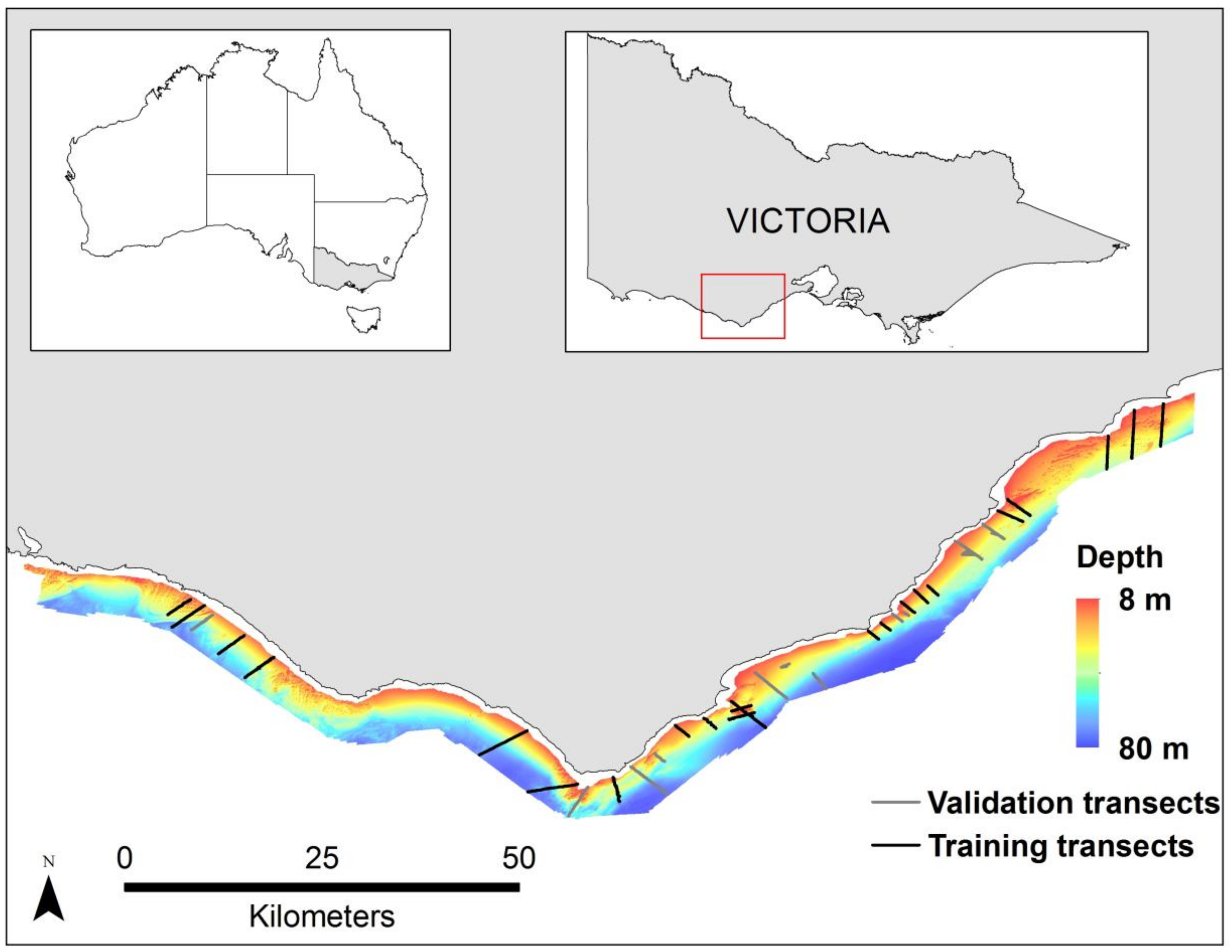
The study area encompasses 700 square kilometers surrounding Cape Otway in Southeast Australia with full MBES data coverage in depths ranging from 10–80 m and is located along the Bass Strait and Western Bass Strait ecoregions [39]. The Cape Otway coastline is highly exposed due to its orientation to prevailing southwesterly ocean swells (Figure 1). In the east, the site is characterized by large sandy embayments with headland reef systems extending offshore. To the south and west, complex rocky reef systems extend offshore from an erosional shoreline of cliffs and limestone stacks [40]. Shallow reefs support diverse communities dominated by canopy forming kelps or open areas of red seaweeds. Deeper reefs in the region are generally populated by diverse sessile invertebrates or crustose coralline algae [40].
2.2. MBES Data Collection and Processing
MBES data were collected from 2006–2008 using a Reson Seabat 8101 MBES operating at a frequency of 240 kHz aboard the Australian Maritime College vessel R.V. Bluefin. Vessel positon was determined by differential GPS (DGPS) and motion values were captured by a POS-MV motion sensor recording heave, pitch, roll and yaw with an accuracy of ±0.02 degrees. Bathymetry was collected with a horizontal accuracy of ±0.3 m. Bathymetry and backscatter values were processed using Starfix suite 7.1 and University of New Brunswick (UNB1) algorithm. The processed bathymetry and backscatter data were gridded to 2.5 m resolution.
For analysis, we merged the rasters from each survey into a single bathymetry and a single backscatter surface using ENVI 5.3.1 [41]. ENVI was used to stitch and fill any holes in the dataset using Delaunay triangulation of values from the surrounding surface. Once the two surfaces were created a mask was used to exclude any islands in the data and clip both surfaces to common extents. We extracted derivatives using ENVI and ArcMap 10.4.1 [42] that represent variability in seafloor structure (Table 1).
Derivatives were created from the bathymetry and backscatter products based on methods from previous habitat mapping studies [3,19] (Table 1). To gain a better understanding of the influence of scale on model results, each derivative was created at an analysis kernel size ranging 3 × 3 to 21 × 21 pixels. This resulted in products for each of the 14 seafloor derivatives at analysis scales of 3, 5, 7, 9, 11, 13, 15, 17, 19 and 21 pixels, a total of 140 derived products.
2.3. Groundtruth Collection and Classification
Over 180 linear kilometers of towed video groundtruth data were collected by the Deakin Marine Mapping Group using a custom towed-video system (for details see [19]). The Cape Otway dataset is extensive and combines data collected over two years across 30 shore-normal transects. During tows, the camera system was piloted via live-stream video from an umbilical and kept ~1 m off the seafloor resulting in a field of view of roughly 2 m × 2 m. Camera position was recorded via an ultra-short baseline transponder and the vessel’s DGPS.
The towed video dataset was classified using the Combined Biotope Classification Scheme (CBiCS) which has been adopted by the Department of Environment, Land, Water and Planning (Victorian Government, Australia) [45]. The video data was segmented into multiple categories of habitat type for each of the CBiCS hierarchies, based on observations of biota, substrata, geoform, exposure, and biogeographic region [45]. CBiCS uses components of the Joint Nature Conservation Committee-European Nature Information System (JNCC-EUNIS [46]), and United States Coastal and Marine Ecological Classification System (CMECS [47]), with a total of six hierarchical levels representing the biotic component [48]. Three levels of the scheme were used in this study; broad habitat classes (BC2), habitat complexes (BC3), and biotope complexes (BC4) (Table 2). CBiCS also provides classifications for biotopes (BC5) and morphospecies (BC6), however, they were not explored due to the large number of rare classes with limited observations for training and validation data sets within the study area.
In order to limit spatial autocorrelation between the training and validation sets, transects were chosen at random, 20 for training and 10 for validation. There were 14,785 observations in the training data set and 7835 observations in the validation data set. To ensure only a single towed video observation represented each raster cell the observation data were thinned with a buffer of 4 m between observations.
2.4. Wave Exposure Model
As a surrogate for wave exposure, we used a fine-scale (60 m) estimation of wave induced orbital velocities of the seabed. The model was created using the WaveWatch III global hindcast model downscaled to a regional spectral wave model using the high-resolution bathymetric surface [18]. Wave-induced orbital velocities were transferred to the seafloor using linear wave theory (for more detailed information see [18]). Bayesian kriging was used to resample the wave exposure surface to a resolution of 2.5 m and mean kernel size analysis was performed to produce surfaces at identical scales to those defined in Section 2.2.
2.5. Statistical Approaches
2.5.1. Data Analysis
The Random Forests (RF) ensemble classification approach was used to derive rule-based relationships between geophysical derivatives and corresponding observational data using the “randomForest” package in R [49]. RF is a machine learning modelling technique that uses tree-type classifiers and bootstrap aggregation based on subsets of the input data [50]. The benefits of using the RF classification approach are that it reduces the chance of overfitting the model by including the results of multiple trees from bootstrap samples of the training data, and measures of variable importance to model accuracy can be derived [51]. RF also keeps bias low via random predictor selection. RF have been shown to perform well when compared with other rule-based classification approaches, as demonstrated by Stephen and Diesing [52], who reported that tree-based methods, including RF, performed best when predicting sediment classes from acoustic and groundtruth data sets.
Parameters for the optimal number of predictors randomly selected at each split (mtry), and the optimal number of trees within models (ntree) were assessed for each of the three hierarchical models using a repeated K-fold cross-validation routine in the R package ‘caret’ [53]. Model parameters mtry and ntree were subsequently set at values of 5 and 300 respectively for the three hierarchical models used in the study.
2.5.2. Variable Importance
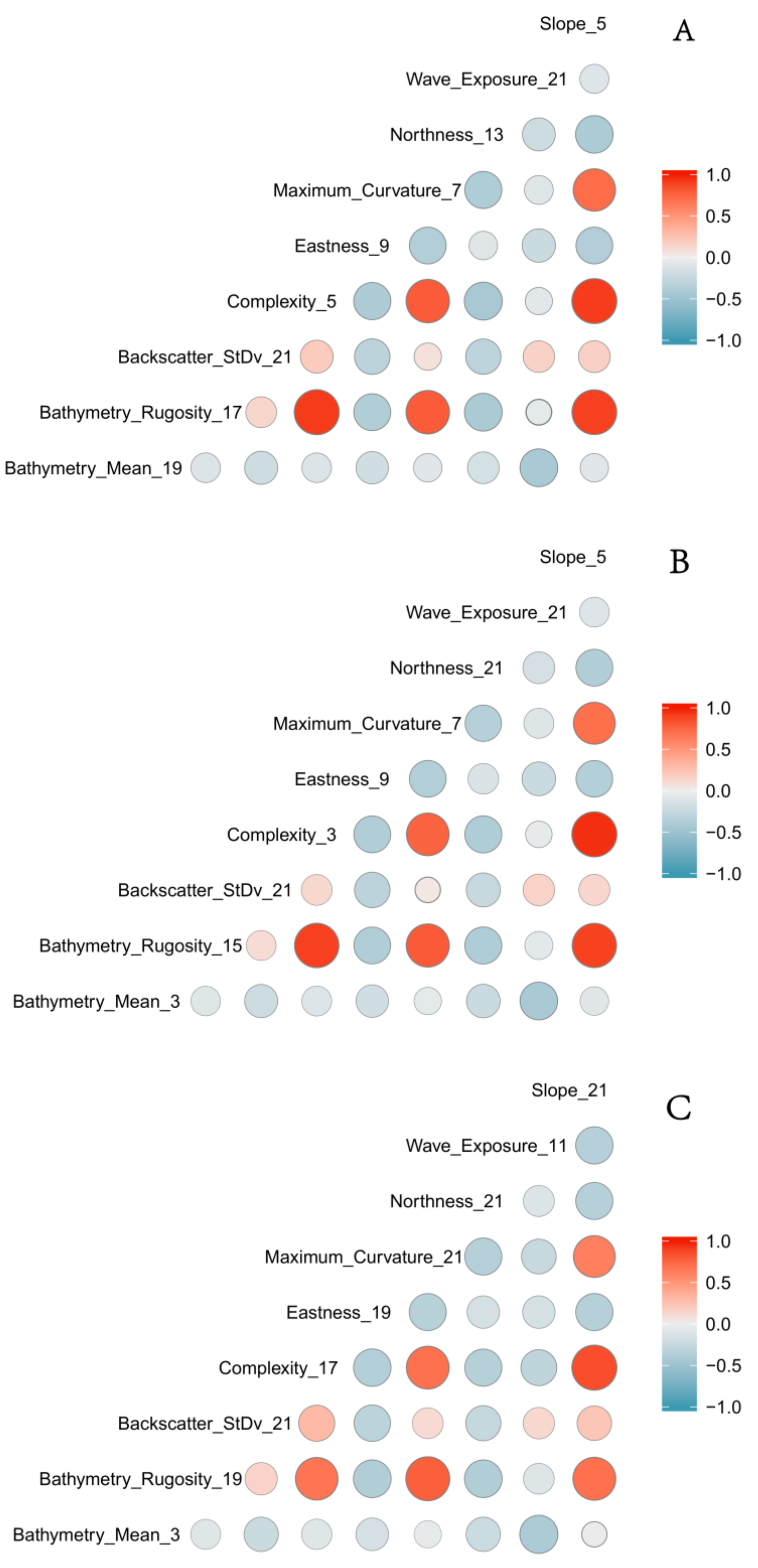
Variable importance was obtained by randomly permuting each predictor value in the “out of bag” (OOB) observations for each tree. The error rate for classification is calculated for each tree in the model, and the same is done for each predictor variable. The differences between the two errors are averaged over all trees and normalized using the standard deviation from the differences. Predictors for each of the three hierarchical models were chosen based on variable importance without repetition (i.e., if two variables with analysis kernels of 21 and 19 pixels were ranked equally only one was included). Predictors with a Pearson product-moment correlation value greater than 0.8 were not retained for model runs (Figure 3). See Table 3 for predictors used in RF modelling for the three hierarchical models.
2.5.3. Predictive Mapping
RF models were used to predict the final classified habitat maps using the “ModelMap” package in R [54]. Model accuracies were determined by creating confusion matrices comparing the predicted classifications with the validation dataset providing overall accuracies, kappa statistics and measures of within class model performance (sensitivity and specificity) for each model using the “caret” package in R. The Kappa statistic (K̂) measures the agreement between an observed accuracy and an expected (values ranging from −1 to 1), but differs from a simple percent agreement calculation as it considers the agreement occurring by chance [55].
3. Results
3.1. Habitat Suitability Maps
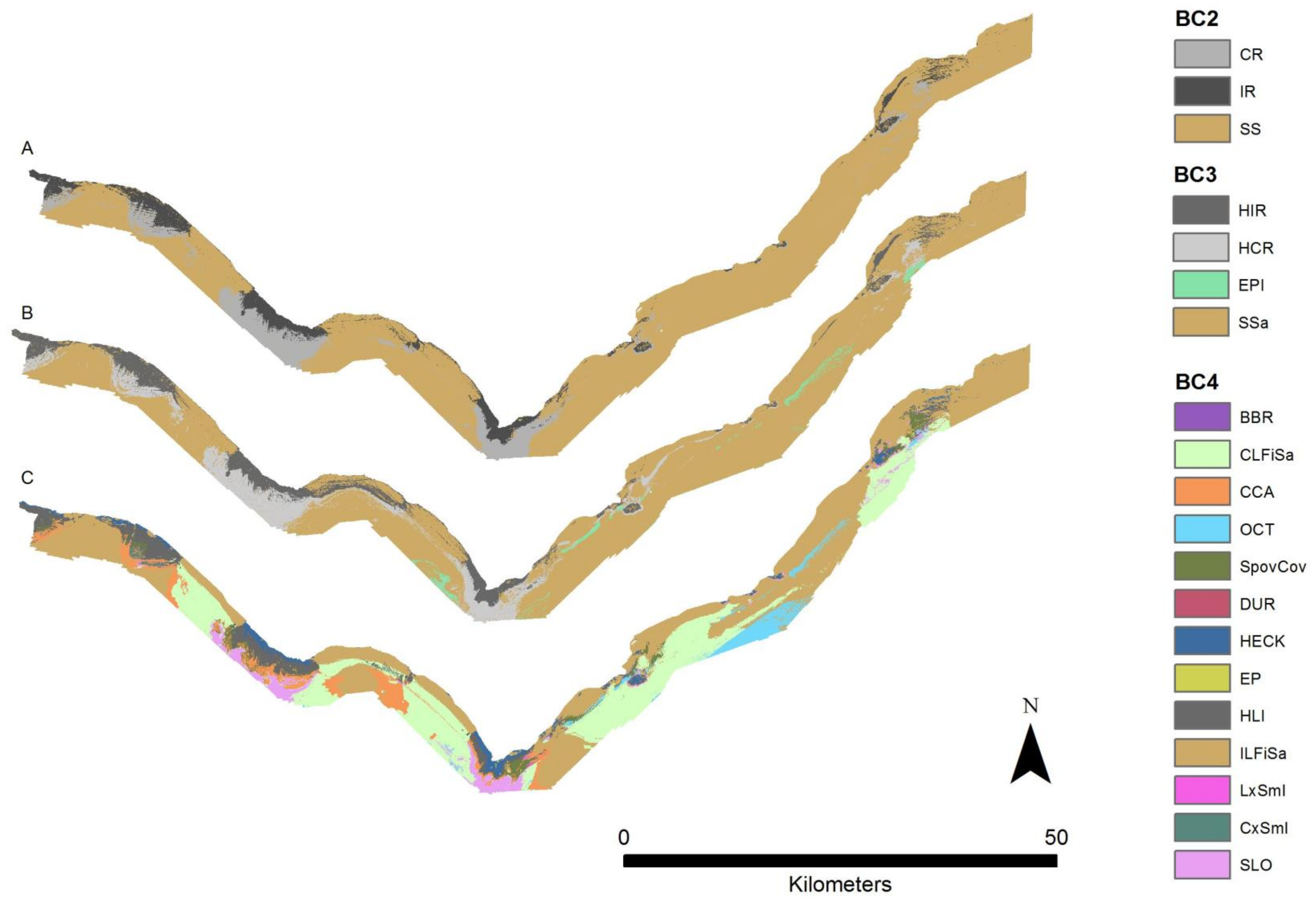
The results of the benthic habitat maps indicate at the BC2 hierarchy the Cape Otway site is characterized by sublittoral sediments with extensive circalittoral rock and infralittoral rock more dominant west of the cape (Figure 4). The habitat map for BC3 is similar to BC2, but has an additional class, non-reef sediment epibenthos, which is present in small patches west of the cape.
The smallest class observed in groundtruth for BC4 was high energy Durvillaea communities located in the south of the cape at depths less than 16 m. High energy Ecklonia-Phyllospora biotope complexes were distributed in patches at a mean depth of 19 m ± 2 m. High energy Ecklonia biotope complexes had a mean depth of 22 m ± 4 m within reefs along the western side of Cape Otway heads. The most dominant class, accounting for 71% of the infralittoral hierarchy, was the class high energy lower infralittoral zone. Biotopes included in the biotope complex high energy lower infralittoral zone for this study area are Ecklonia radiata park, and foliose red algae with sessile invertebrates.
The circalittoral zone, classified at the level of BC4, contained the highest number of biotope complexes. Bushy bryozoan-dominated communities were primarily distributed south of the headlands with a mean depth of 35 m ± 2 m. The biotope complexes of high energy circalittoral rock with seabed covering sponges, low complexity circalittoral rock with non-crowded erect sponges, and moderate to high energy circalittoral rock with seabed covering sponges were found at a mean depth of 42 m ± 6 m. Sandy low-profile reef wave surge communities with sand trapped around sponges were found throughout the site at a mean depth of 47 m ± 8 m. The most dominant biotope complex by area, accounting for 45% of the circalittoral habitat in the study area, was crustose coralline algal communities with combinations of thallose red algae and scattered sponges on high energy circalittoral rock at a mean depth of 48 m ± 8 m.
Two of the three classes, infralittoral and circalittoral fine sand, within the sublittoral sediment hierarchy represented 72% (by area) of the BC4 benthic habitat map. The remaining class was “erect octocorals on sediment” and was present east of the heads at a mean depth of 65 m ± 15 m.
3.2. Hierarchical Comparison
Three benthic habitat maps, one for each hierarchical level, were assessed comparing predicted classes to a validation dataset comprised of spatially independent transects not used in model development. The classification for BC2 performed best with an overall accuracy of 87.4% and a Kappa statistic of 0.59 (Table 4). Hierarchical models for BC3 and BC4 had overall accuracies of 69.7% (K̂ = 0.31) and 39.9% (K̂ = 0.16), respectively.
Class specific classification accuracies for BC2 were generally good with all three classes predicting at 60% or higher. Within BC2 sublittoral sediment (SS) performed the best at 91.9% while circalittoral rock (CR) and infralittoral rock (IR) performed moderately at 63.5% and 72.7% respectively (Table 4). The next level in the hierarchy, BC3, predicted three classes accurately with high-energy infralittoral rock (HIR), high-energy open-coast circalittoral rock (HCR) and sublittoral sand and muddy sand (SSa) performing well at 70.6%, 63.4% and 86.3%, respectively. The model failed to accurately differentiate any of the non-reef sediment epibenthos which was incorrectly classified predominately as sublittoral sand and muddy sand (Table 5). As the number of hierarchy levels increased the class specific accuracies typically decreased, with seven of the 13 classes of BC4 consistently incorrectly classified. Five of the seven classes consistently misclassified were from the high-energy circalittoral rock habitat complex: high-energy circalittoral rock with seabed covering sponges, bushy bryozoan-dominated communities, crustose coralline algal communities with combinations of thallose red algae and scattered sponges on high-energy circalittoral rock, low complexity circalittoral rock with non-crowded erect sponges, and moderate to high complexity circalittoral rock with seabed covering sponges. The two other misclassified biotope complexes were from the high-energy infralittoral rock habitat complex: high-energy Durvillaea communities, and high-energy Ecklonia-Phyllospora communities (Table 6). The remaining classes varied in their accuracies with high-energy Ecklonia communities (HECK) preforming the best at 97.1%.
3.3. Variable Importance
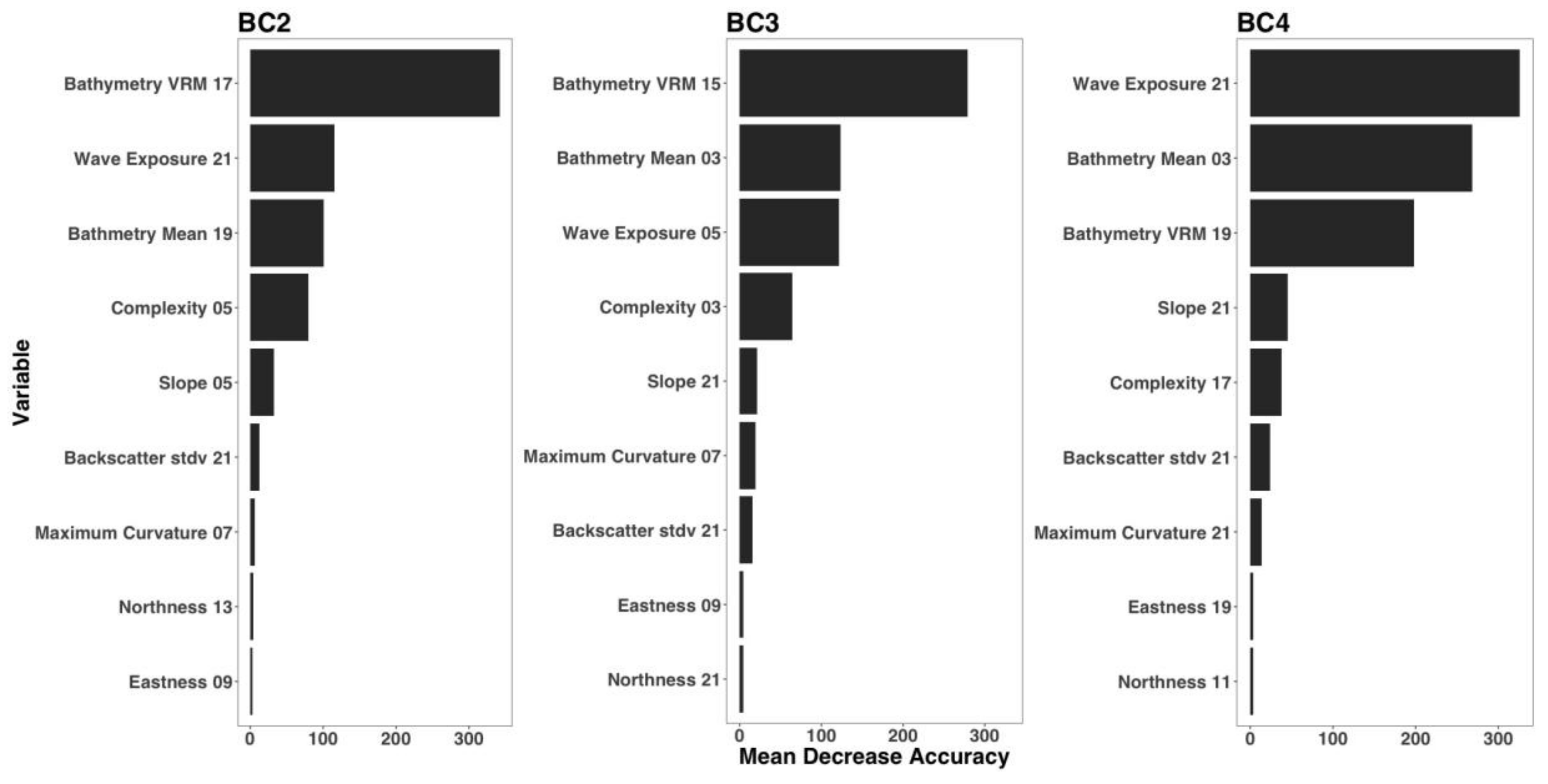
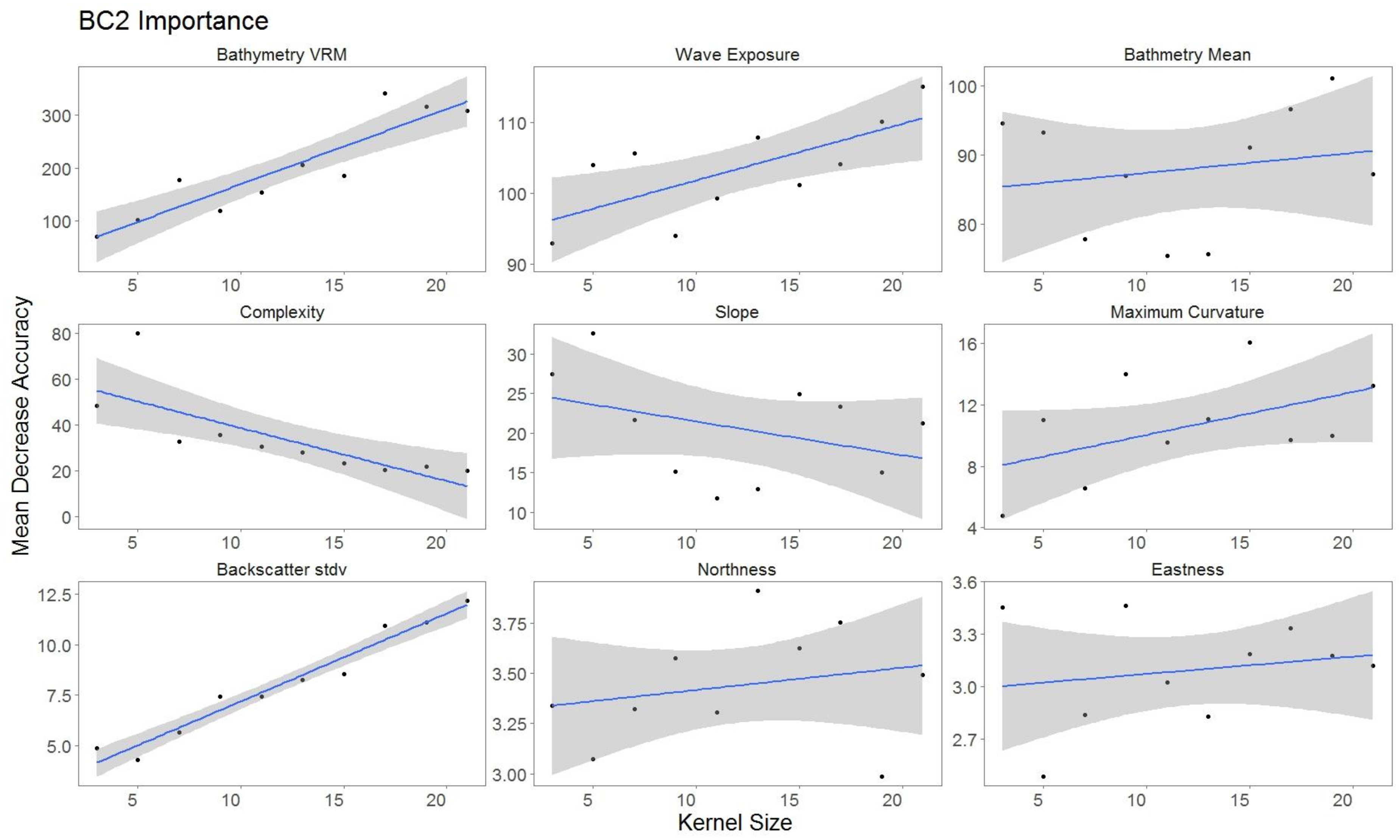
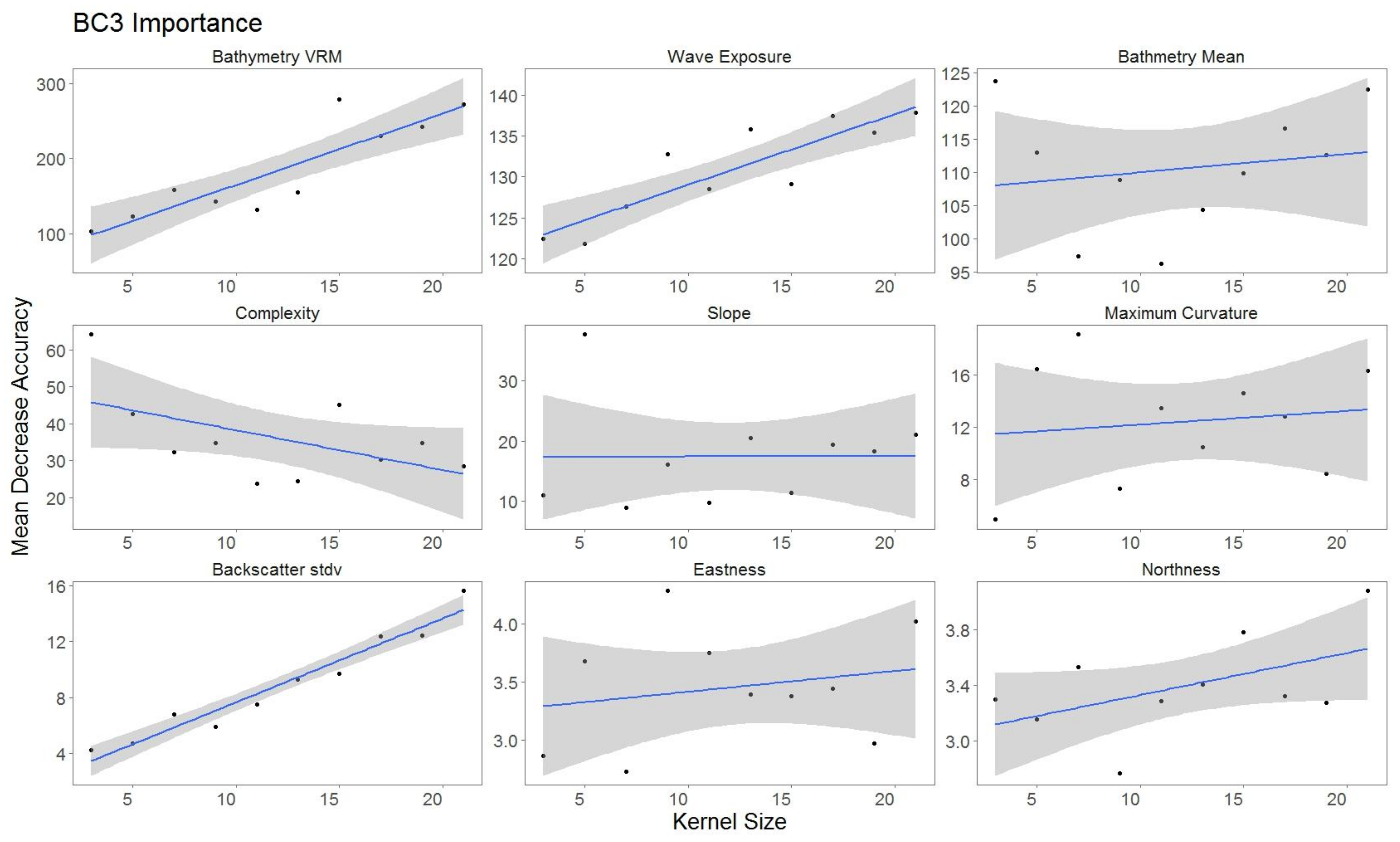
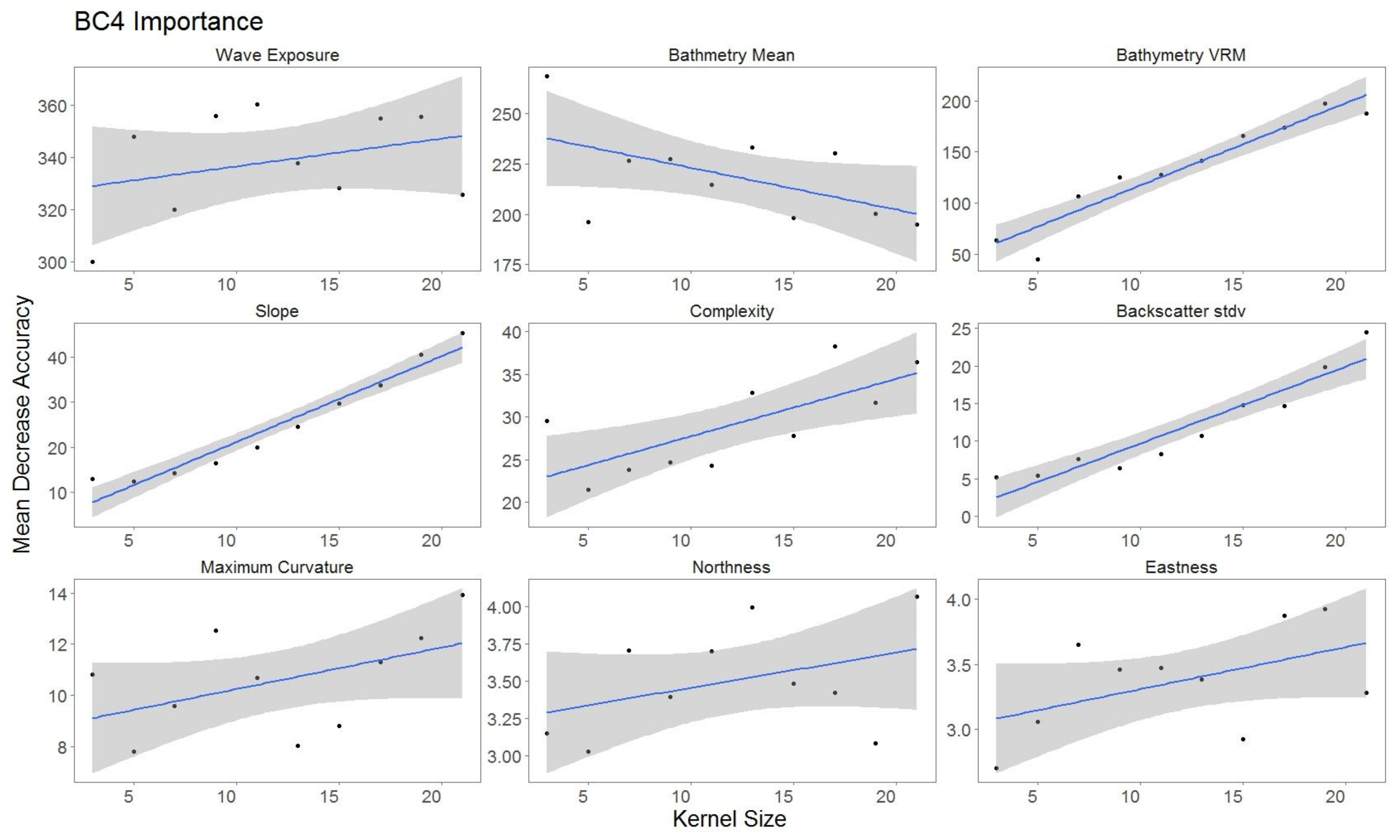
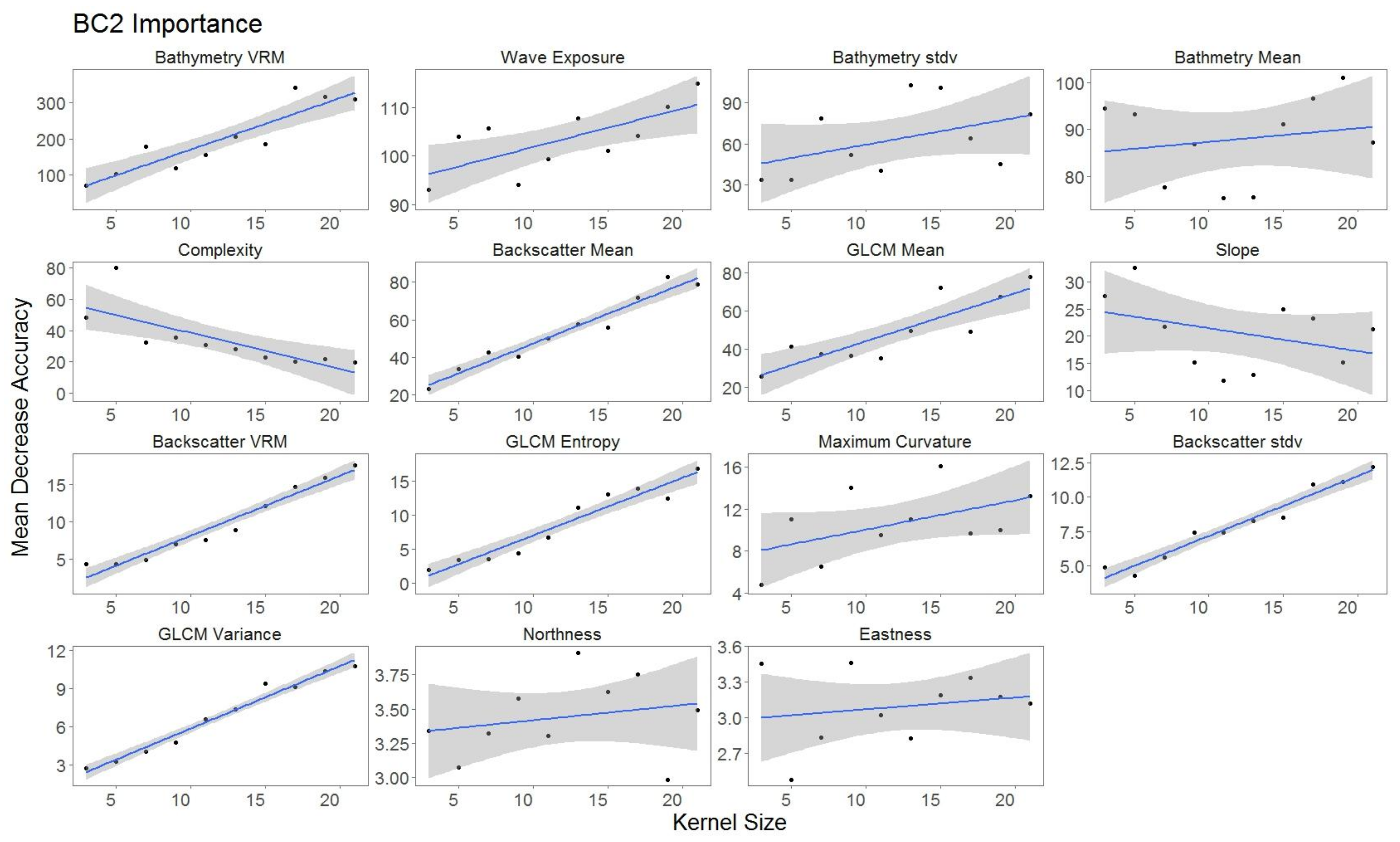
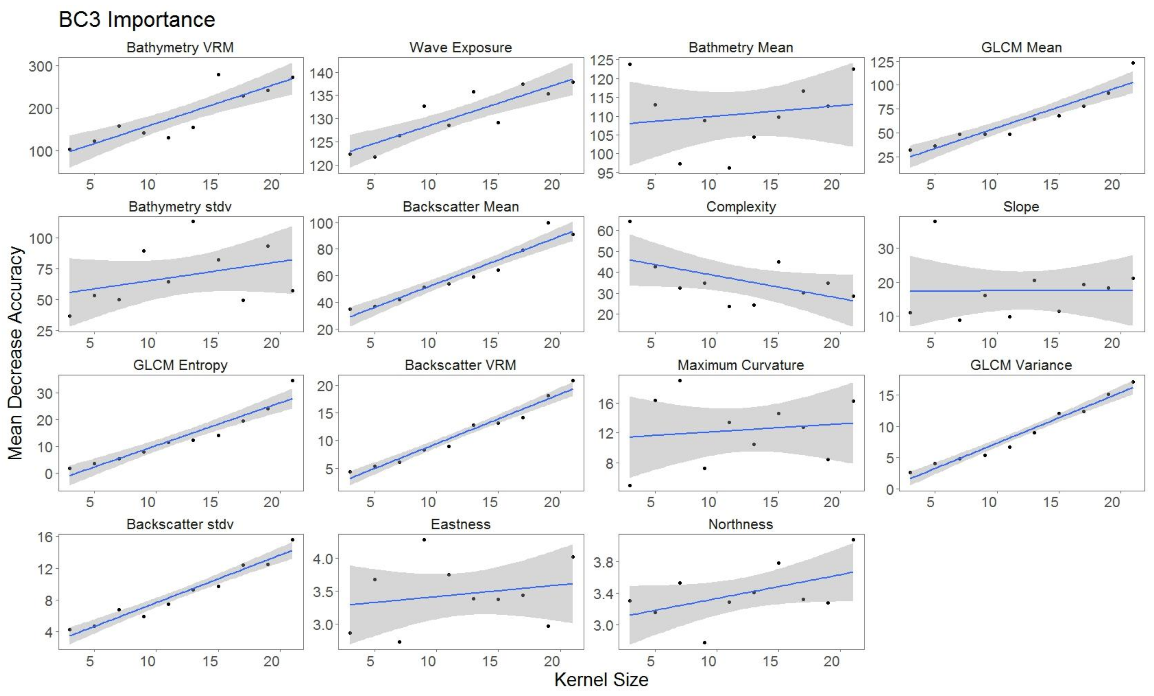
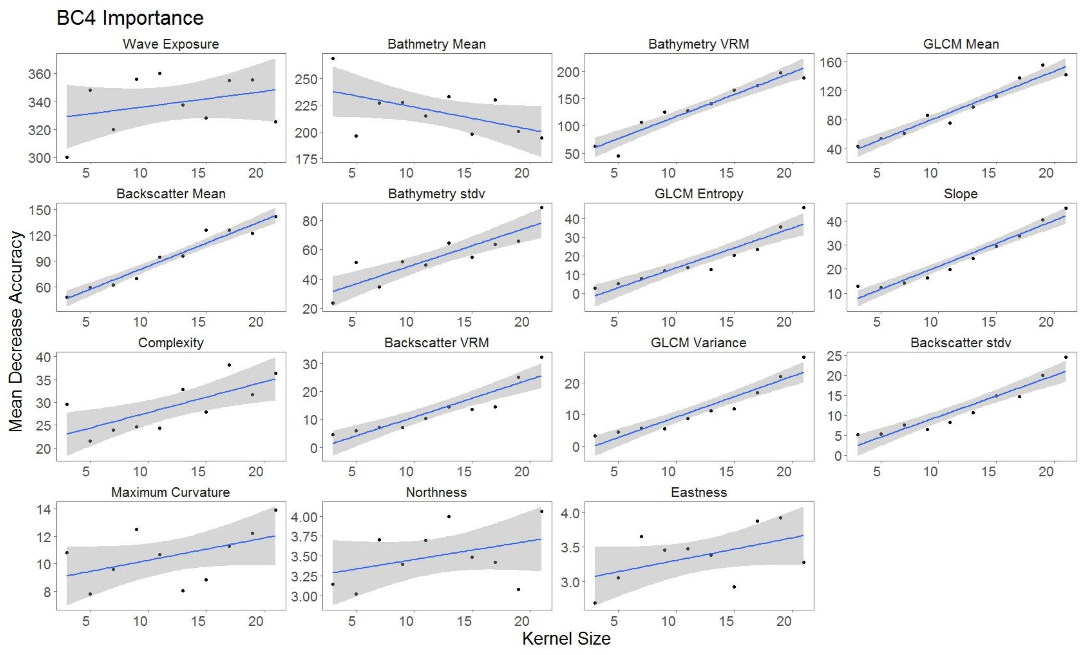
For each hierarchical model, variable importance was ranked using the mean decrease in accuracy metric (Figure 5). A larger value for mean decrease in accuracy indicates that the environmental predictor was more important during the classification process. Wave exposure performed the best for hierarchical level BC4. Bathymetry rugosity (VRM) performed best for hierarchal levels BC2 and BC3. Backscatter mean, backscatter rugosity (VRM), backscatter standard deviation, GLCM entropy, GLCM mean, GLCM variance and maximum curvature shared positive linear trends across predictor scale and between each hierarchy (Figure A1, Figure A2,Figure A3, Figure 6, Figure 7 and Figure 8). Eastness and northness had no patterns in predictor scale or between hierarchical scale. Bathymetry mean performed well across all predictor scales and hierarchies, favoring finer scales for BC4. Bathymetry standard deviation for BC2 and BC3 favored predictor scales towards the mid-range of pixel kernel size (11–15) while BC4 displayed a positive linear relationship (Figure A1, Figure A2 and Figure A3). At coarse hierarchical levels slope favored finer scales, while at finer hierarchical levels slope favored broader scales. In BC2 the relationship between complexity and variable scale favored finer scales with BC3 showing no pattern, and BC4 favoring broader scales.
4. Discussion
Numerous habitat mapping studies have tested the importance of environmental predictor scale when creating habitat maps [2,3,56]. There have also been a number of studies, primarily terrestrial, that have examined the effects of hierarchical classifications on habitat prediction [33,35,36]. In this study, we tested both hierarchical and environmental variable scale in a marine environment, using MBES and terrain derivatives, and demonstrate their importance in developing statistical relationships between observations and geophysical products to create benthic habitat maps.
4.1. Impact of Classification Hierarchy on Model Performance
We observed a decrease in map accuracy at increasing levels of complexity of a hierarchical classification scheme. The lower accuracy of the hierarchical models as more classes were added in BC3 and BC4 is likely due to the decrease in samples per class and increased complexity of the classification task, a common challenge experienced across many studies (see review [57]). Additionally, as class complexity increased, some rarer habitats were under represented, with too few samples for rigorous model training and validation. Mumby et al. [38] found similar results using a hierarchical cluster analysis to predict coral reefs habitats according to three levels (broad, intermediate, and fine) of hierarchy across five different satellite sensors [38]. They found a significant decrease in accuracy between broad to fine descriptive resolutions [38]. Capolsini et al. [58] found a similar pattern in decreased accuracy when using more classes to define coral reef habitats in South Pacific Islands.
According to benchmarks established by Landis et al. [59] kappa values in the present study indicate that BC2 had moderate strength of agreement, BC3 had fair strength of agreement and BC4 displayed slight strength of agreement. The moderate and fair agreement for BC2 and BC3 provide confident results. The slight strength in agreement for BC4 is likely due to multiple rare and similar classes, with two of the classes having 10 observations and the remainder having similar characteristics; all located on circalittoral rock, with either crustose coralline algal communities, sponges, or bryozoans.
Sediment classes with no visible epibiota; SS, SSa, and ILFiSa were consistently accurately classified, likely because sediment morphology displays patterns that are readily discernible from reef using MBES derivatives [1,60]. In the hierarchical level BC3, the model failed to accurately classify any of the sediment classes containing visible epibenthos. This may reflect poor class separability using acoustic methods, as demonstrated by Freitas et al. [61], who found that acoustic methods had difficulty separating grain sizes between fine and very fine sand. Reef classes had, in general, lower accuracies. This is possibly due to low profile reefs in the study area having sand veneers making them difficult to discern using MBES derivatives. Classes with similar biotic components, namely crustose coralline algal communities, and seabed/erect sponges, were misclassified throughout BC4. This finding is similar to a predictive modelling study conducted by Che Hasan et al. [62], which found that misclassification occurred between similar biota classes (i.e., mixed brown algae, mixed brown and invertebrates) because they shared many acoustic properties due to similar species compositions and substratum types. Some classes are rare, with low density biota making it difficult to discern from surrounding acoustic signatures.
4.2. Impact of Variable Scale
A common finding across all three hierarchies was the importance of wave exposure in reducing classification uncertainty. Wave exposure was the highest ranked variable in the BC4 model and was the second highest variable in the BC2 and BC3 hierarchical models, which is unsurprising given the strong east-west exposure gradient at the site. Characteristics used to determine biotope classes often include exposure level, reinforcing the desirability of incorporating variables describing local exposure gradients in habitat maps [63]. Our results align with findings from previous studies where oceanographic features and seafloor habitat variables were incorporated into habitat models [18,64]. Rattray et al. [18] found that incorporating wave exposure as a variable in habitat mapping significantly increased model accuracy when compared to models derived using MBES derivatives alone. Downscaling the original hindcast model using Bayesian kriging likely weakened the mean decrease in accuracy relationship between each scale because the original scale of the model is coarser than the coarsest scale extracted.
Seafloor habitat variables derived from bathymetry rugosity (VRM) and backscatter standard deviation shared common trends as both predictors were important across hierarchies. Another pattern observed across hierarchies was the increasing importance of environmental predictors derived from the backscatter layer as scale increased (Figure A1, Figure A2 and Figure A3), while predictors derived from bathymetry displayed weaker trends. An explanation for this pattern may be the larger number of artefacts in the backscatter layer in comparison to bathymetry. Deriving backscatter derivatives at broader scales potentially reduces speckle and nadir noise common in backscatter mosaics [19].
Within each classification hierarchy most environmental predictors showed increased importance at broader scales of analysis, with a few exceptions; for example, eastness, northness, bathymetry mean and complexity at hierarchical models BC2 and BC3 were more important at finer scales. In similar multiscale studies, a combination of fine and broad-scale variables were found to be the best predictors of bird habitat [65] and macrofaunal habitat [22]. This reflects findings in the marine environment indicating that species/habitat associations may be based on a combination of both broad-scale and fine-scale variables [66]. However, when habitats are best represented by broad-scale variables a previous study by Wilson et al. [3] found that there may be an upper limit to the scale of analysis before variable importance decreases. Scale importance in our study did not appear to reach any upper limits for most variables; suggesting future studies should examine derivatives at even broader scales for model input.
Importance of scale is likely site dependent and driven by the heterogeneity of the seabed and size of the study area [67,68]. Results from this study provide an example from a highly exposed, temperate coastline, which may be representative of other temperate sites. Using the methodology described here, the effect of scale on classification can be explored and applied to other study areas. Predictive habitat maps based on small class sample sizes are unlikely to be as accurate as those based on classes with large samples, especially when class characteristics share similarities with surrounding classes [67,68], or when predictors do not adequately represent processes driving biotic distribution. Groundtruth surveys are typically carried out after the collection and processing of MBES bathymetry and backscatter. Using unsupervised classification techniques to guide collection of observation data is a logical first step to ensuring adequate sample sizes across classes of interest. For example, Przeslawski and Foster [69], suggest that transect length should be dependent on the spatial properties of the target biota, using short transects where the biota has large spatial autocorrelation and using long transects where the biota has small spatial autocorrelation. In an effort to reduce spatial autocorrelation we split our observations into training and validation by randomly selecting transects. This was not ideal and likely had a negative impact on model accuracy. Several classes from the BC3 and BC4 levels were only present in a single transect, resulting in either no training or validation points for some classes, thus were excluded from the model.
5. Conclusions
Advances in MBES technology have provided products at increasing resolution, however, studies exploring the impact of variable scale on the habitat mapping process have been limited. When assessing variable importance across multiple scales, our study generally shows positive trends towards broader scale variables. We demonstrate that predictor scale is important for improving map accuracy and suggest multiscale analysis to limit user bias when selecting variable scales for analysis as they are likely to be site specific, which is driven by the heterogeneity of the seascape.
The number of predictive classes and the ability to differentiate between them accurately is a key consideration when deriving benthic habitat maps. Using a hierarchical classification approach for model prediction, we found as the number of predictive classes increased model accuracy decreased. Classification schemes are not necessarily designed with predictive mapping in mind and can result in classes sharing similar abiotic characteristics that can be difficult to differentiate using acoustic approaches. Therefore, classification schemes that incorporate appropriate levels for accurate predictive mapping that aligns with management objectives are desirable.
Rare classes pose a challenge for predictive habitat modelling, because capturing an adequate number of samples when collecting groundtruth data is difficult. For future studies we recommend considering the tradeoff between statistical rigor and useful habitat maps by using a combination of automated and manual digitization of rare classes. In conclusion, this study brings attention to hierarchical classifications and the importance of using multiscale approaches when classifying benthic habitats.
Acknowledgments
This work was supported by the National Heritage Trust and Caring for Country as part of the Victorian Marine Habitat Mapping Project with project partners Glenelg Hopkins Catchment Management Authority, Department of Environment and Primary Industries, Parks Victoria, University of Western Australia and Fugro Survey. We thank the crew from the Australian Maritime College research vessel Bluefin, which was used for the multibeam data collection. We also thank the crew from Deakin University research vessel Courageous II for assisting Daniel Ierodiaconou & Alex Rattray collecting the towed video data used in this project. Towed video was classified by Australian Marine Ecology and Fathom Pacific using CBiCS under a project funded by the Department of Environment, Land, Water and Planning. Multibeam bathymetry and classified towed video data was accessed via the Victoria Marine Data Portal, available online: https://vmdp.deakin.edu.au/ (accessed 2 April 2018). We would like to thank Matt Edmunds and Adrian Flynn for providing comments on the manuscripts first draft and for their contributions in the creation of CBiCS. Alex Rattray and Mary Young were supported by the Victorian Marine Habitat Mapping Program with funds through Department of Environment, Lands Water and Planning, Parks Victoria and Australian National Data Services (ANDS) through funding from the Australian Government’s National Environmental Science Programme.
Author Contributions
Daniel Ierodiaconou conceived the project and led the fieldwork. Peter Porskamp led the analyses and writing with contributions from Daniel Ierodiaconou, Alex Rattray and Mary Young.
Conflicts of Interest
The authors declare no conflict of interest.
Appendix A
Figure A1.
Variable importance BC2 sorted by derivatives in order of importance. GLM trend represented in blue. Gray area represents 95% confidence interval for predictions.
Figure A1.
Variable importance BC2 sorted by derivatives in order of importance. GLM trend represented in blue. Gray area represents 95% confidence interval for predictions.

Figure A2.
Variable importance BC3 sorted by derivatives in order of importance. GLM trend represented in blue. Gray area represents 95% confidence interval for predictions.
Figure A2.
Variable importance BC3 sorted by derivatives in order of importance. GLM trend represented in blue. Gray area represents 95% confidence interval for predictions.

Figure A3.
Variable importance BC4 sorted by derivatives in order of importance. GLM trend represented in blue. Gray area represents 95% confidence interval for predictions.
Figure A3.
Variable importance BC4 sorted by derivatives in order of importance. GLM trend represented in blue. Gray area represents 95% confidence interval for predictions.

References
- Brown, C.J.; Smith, S.J.; Lawton, P.; Anderson, J.T. Benthic habitat mapping: A review of progress towards improved understanding of the spatial ecology of the seafloor using acoustic techniques. Estuar. Coast. Shelf Sci. 2011, 92, 502–520. [Google Scholar] [CrossRef]
- Lecours, V.; Devillers, R.; Schneider, D.; Lucieer, V.; Brown, C.; Edinger, E. Spatial scale and geographic context in benthic habitat mapping: Review and future directions. Mar. Ecol. Prog. Ser. 2015, 535, 259–284. [Google Scholar] [CrossRef]
- Wilson, M.F.J.; O’Connell, B.; Brown, C.; Guinan, J.C.; Grehan, A.J. Multiscale Terrain Analysis of Multibeam Bathymetry Data for Habitat Mapping on the Continental Slope. Mar. Geodesy 2007, 30, 3–35. [Google Scholar] [CrossRef]
- Diesing, M.; Mitchell, P.; Stephens, D. Image-based seabed classification: What can we learn from terrestrial remote sensing? ICES J. Mar. Sci. J. Cons. 2016, 73, 2425–2441. [Google Scholar] [CrossRef]
- Lemme, M.C.; Koppens, F.H.L.; Falk, A.L.; Rudner, M.S.; Park, H.; Levitov, L.S.; Marcus, C.M. Gate-Activated Photoresponse in a Graphene p–n Junction. Nano Lett. 2011, 11, 4134–4137. [Google Scholar] [CrossRef] [PubMed]
- Engle, V.D.; Summers, J.K. Latitudinal gradients in benthic community composition in Western Atlantic estuaries. J. Biogeogr. 1999, 26, 1007–1023. [Google Scholar] [CrossRef]
- Wernberg, T.; Smale, D.A.; Tuya, F.; Thomsen, M.S.; Langlois, T.J.; de Bettignies, T.; Bennett, S.; Rousseaux, C.S. An extreme climatic event alters marine ecosystem structure in a global biodiversity hotspot. Nat. Clim. Chang. 2013, 3, 78–82. [Google Scholar] [CrossRef]
- Gattuso, J.-P.; Gentili, B.; Duarte, C.M.; Kleypas, J.A.; Middelburg, J.J.; Antoine, D. Light availability in the coastal ocean: Impact on the distribution of benthic photosynthetic organisms and contribution to primary production. Biogeosci. Discuss. 2006, 3, 895–959. [Google Scholar] [CrossRef]
- Anthony, K.; Ridd, P.V.; Orpin, A.R.; Larcombe, P.; Lough, J. Temporal variation of light availability in coastal benthic habitats: Effects of clouds, turbidity, and tides. Limnol. Oceanogr. 2004, 49, 2201–2211. [Google Scholar] [CrossRef]
- Bax, N.; Kloser, R.; Williams, A.; Gowlett-Holmes, K.; Ryan, T. Seafloor habitat definition for spatial management in fisheries: A case study on the continental shelf of southeast Australia. Oceanol. Acta 1999, 22, 705–720. [Google Scholar] [CrossRef]
- Roff, J.C.; Taylor, M.E.; Laughren, J. Geophysical approaches to the classification, delineation and monitoring of marine habitats and their communities. Aquat. Conserv. Mar. Freshw. Ecosyst. 2003, 13, 77–90. [Google Scholar] [CrossRef]
- McArthur, M.A.; Brooke, B.P.; Przeslawski, R.; Ryan, D.A.; Lucieer, V.L.; Nichol, S.; McCallum, A.W.; Mellin, C.; Cresswell, I.D.; Radke, L.C. On the use of abiotic surrogates to describe marine benthic biodiversity. Estuar. Coast. Shelf Sci. 2010, 88, 21–32. [Google Scholar] [CrossRef]
- Kostylev, V.E.; Erlandsson, J.; Ming, M.Y.; Williams, G.A. The relative importance of habitat complexity and surface area in assessing biodiversity: Fractal application on rocky shores. Ecol. Complex. 2005, 2, 272–286. [Google Scholar] [CrossRef]
- Lecours, V.; Devillers, R.; Simms, A.E.; Lucieer, V.L.; Brown, C.J. Towards a framework for terrain attribute selection in environmental studies. Environ. Model. Softw. 2017, 89, 19–30. [Google Scholar] [CrossRef]
- Mitchell, P.J.; Monk, J.; Laurenson, L. Sensitivity of fine-scale species distribution models to locational uncertainty in occurrence data across multiple sample sizes. Methods Ecol. Evol. 2017, 8, 12–21. [Google Scholar] [CrossRef]
- Ierodiaconou, D.; Monk, J.; Rattray, A.; Laurenson, L.; Versace, V.L. Comparison of automated classification techniques for predicting benthic biological communities using hydroacoustics and video observations. Cont. Shelf Res. 2011, 31, S28–S38. [Google Scholar] [CrossRef]
- Ierodiaconou, D.; Laurenson, L.; Burq, S.; Reston, M. Marine benthic habitat mapping using Multibeam data, georeferencedvideo and image classification techniques in Victoria, Australia. J. Spat. Sci. 2007, 52, 93–104. [Google Scholar] [CrossRef]
- Rattray, A.; Ierodiaconou, D.; Womersley, T. Wave exposure as a predictor of benthic habitat distribution on high energy temperate reefs. Front. Mar. Sci. 2015, 2. [Google Scholar] [CrossRef]
- Ierodiaconou, D.; Schimel, A.C.G.; Kennedy, D.; Monk, J.; Gaylard, G.; Young, M.; Diesing, M.; Rattray, A. Combining pixel and object based image analysis of ultra-high resolution multibeam bathymetry and backscatter for habitat mapping in shallow marine waters. Mar. Geophys. Res. 2018. [Google Scholar] [CrossRef]
- Hasan, R.; Ierodiaconou, D.; Monk, J. Evaluation of Four Supervised Learning Methods for Benthic Habitat Mapping Using Backscatter from Multi-Beam Sonar. Remote Sens. 2012, 4, 3427–3443. [Google Scholar] [CrossRef]
- Siwabessy, P.J.W.; Tran, M.; Picard, K.; Brooke, B.P.; Huang, Z.; Smit, N.; Williams, D.K.; Nicholas, W.A.; Nichol, S.L.; Atkinson, I. Modelling the distribution of hard seabed using calibrated multibeam acoustic backscatter data in a tropical, macrotidal embayment: Darwin Harbour, Australia. Mar. Geophys. Res. 2017. [Google Scholar] [CrossRef]
- De Leo, F.C.; Vetter, E.W.; Smith, C.R.; Rowden, A.A.; McGranaghan, M. Spatial scale-dependent habitat heterogeneity influences submarine canyon macrofaunal abundance and diversity off the Main and Northwest Hawaiian Islands. Deep Sea Res. Part II Top. Stud. Oceanogr. 2014, 104, 267–290. [Google Scholar] [CrossRef]
- Bouchet, P.J.; Meeuwig, J.J.; Salgado Kent, C.P.; Letessier, T.B.; Jenner, C.K. Topographic determinants of mobile vertebrate predator hotspots: Current knowledge and future directions: Landscape models of mobile predator hotspots. Biol. Rev. 2015, 90, 699–728. [Google Scholar] [CrossRef] [PubMed]
- Walbridge, S.; Slocum, N.; Pobuda, M.; Wright, D.J. Unified Geomorphological Analysis Workflows with Benthic Terrain Modeler. Geosciences 2018, 8, 94. [Google Scholar] [CrossRef]
- Le Bas, T.P.; Huvenne, V.A.I. Acquisition and processing of backscatter data for habitat mapping—Comparison of multibeam and sidescan systems. Appl. Acoust. 2009, 70, 1248–1257. [Google Scholar] [CrossRef]
- MacMillan, R.A.; Shary, P.A. Chapter 9 Landforms and Landform Elements in Geomorphometry. In Developments in Soil Science; Elsevier: Amsterdam, The Netherlands, 2009; Volume 33, pp. 227–254. ISBN 978-0-12-374345-9. [Google Scholar]
- Lindegarth, M.; Gamfeldt, L. Comparing Categorical and Continuous Ecological Analyses: Effects of “Wave Exposure” on Rocky Shores. Ecology 2005, 86, 1346–1357. [Google Scholar] [CrossRef]
- Bustamante, R.H.; Branch, G.M. Large Scale Patterns and Trophic Structure of Southern African Rocky Shores: The Roles of Geographic Variation and Wave Exposure. J. Biogeogr. 1996, 23, 339–351. [Google Scholar] [CrossRef]
- Hughes, M.G.; Heap, A.D. National-scale wave energy resource assessment for Australia. Renew. Energy 2010, 35, 1783–1791. [Google Scholar] [CrossRef]
- Dartnell, P.; Gardner, J.V. Predicting Seafloor Facies from Multibeam Bathymetry and Backscatter Data. Photogramm. Eng. Remote Sens. 2004, 70, 1081–1091. [Google Scholar] [CrossRef]
- Costello, M. Distinguishing marine habitat classification concepts for ecological data management. Mar. Ecol. Prog. Ser. 2009, 397, 253–268. [Google Scholar] [CrossRef]
- Simboura, N.; Zenetos, A. Benthic indicators to use in Ecological Quality classification of Mediterranean soft bottom marine ecosystems, including a new Biotic Index. Mediterr. Mar. Sci. 2002, 3, 77. [Google Scholar] [CrossRef]
- Guarinello, M.L.; Shumchenia, E.J.; King, J.W. Marine Habitat Classification for Ecosystem-Based Management: A Proposed Hierarchical Framework. Environ. Manag. 2010, 45, 793–806. [Google Scholar] [CrossRef] [PubMed]
- Shumchenia, E.J.; King, J.W. Comparison of methods for integrating biological and physical data for marine habitat mapping and classification. Cont. Shelf Res. 2010, 30, 1717–1729. [Google Scholar] [CrossRef]
- Klijn, F.; de Haes, H.A.U. A hierarchical approach to ecosystems and its implications for ecological land classification. Landsc. Ecol. 1994, 9, 89–104. [Google Scholar] [CrossRef]
- Frissell, C.A.; Liss, W.J.; Warren, C.E.; Hurley, M.D. A hierarchical framework for stream habitat classification: Viewing streams in a watershed context. Environ. Manag. 1986, 10, 199–214. [Google Scholar] [CrossRef]
- Bock, M.; Xofis, P.; Mitchley, J.; Rossner, G.; Wissen, M. Object-oriented methods for habitat mapping at multiple scales—Case studies from Northern Germany and Wye Downs, UK. J. Nat. Conserv. 2005, 13, 75–89. [Google Scholar] [CrossRef]
- Mumby, P.J.; Green, E.P.; Edwards, A.J.; Clark, C.D. Coral reef habitat mapping: How much detail can remote sensing provide? Mar. Biol. 1997, 130, 193–202. [Google Scholar] [CrossRef]
- Department of the Environment and Heritage. A Guide to the Integrated Marine and Coastal Regionalisation of Australia: IMCRA Version 4.0; Australian Government, Department of the Environment and Heritage: Canberra, Australia, 2006; ISBN 978-0-642-55227-3. [Google Scholar]
- Bezore, R.; Kennedy, D.M.; Ierodiaconou, D. The Drowned Apostles: The Longevity of Sea Stacks over Eustatic Cycles. J. Coast. Res. 2016, 75, 592–596. [Google Scholar] [CrossRef]
- ENVI; Exelis Visual Information Solutions: Boulder, CO, USA, 2010.
- ArcGIS; Environmental Systems Research Institute (ESRI): Redlands, CA, USA, 2015.
- Sappington, J.M.; Longshore, K.M.; Thompson, D.B. Quantifying Landscape Ruggedness for Animal Habitat Analysis: A Case Study Using Bighorn Sheep in the Mojave Desert. J. Wildl. Manag. 2007, 71, 1419–1426. [Google Scholar] [CrossRef]
- Haralick, R.M.; Shanmugam, K.; Dinstein, I. Textural Features for Image Classification. IEEE Trans. Syst. Man Cybern. 1973, 3, 610–621. [Google Scholar] [CrossRef]
- Edmunds, M.; Flynn, A. A Victorian Marine Biotope Classification Scheme; Report to Deakin University and Parks Victoria; Australian Marine Ecology Report No. 545; Deakin University: Melbourne, Australia, 2015. [Google Scholar]
- Davies, C.E.; Moss, D.; Hill, M.O. EUNIS Habitat Classification Revised 2004; European Topic Centre on Nature Protection and Biodiversity: Paris, France, 2004; pp. 127–143. [Google Scholar]
- Federal Geographic Data Committee. Coastal and Marine Ecological Classification Standard; FGDC-STD-018-2012; Federal Geographic Data Committee, Marine and Coastal Spatial Data Subcommittee: Reston, VA, USA, 2012. [Google Scholar]
- Eigenraam, M.; McCormick, F.; Contreras, Z. Marine and Coastal Ecosystem Accounting: Port Phillip Bay; State of Victoria Department of Environment, Land, Water and Planning: Victoria, Australia, 2016. [Google Scholar]
- Liaw, A.; Wiener, M. Classification and Regression by randomForest. R News 2002, 2, 18–22. [Google Scholar]
- Breiman, L. Random forests. Mach. Learn. 2001, 45, 5–32. [Google Scholar] [CrossRef]
- Cutler, D.R.; Edwards, T.C.; Beard, K.H.; Cutler, A.; Hess, K.T.; Gibson, J.; Lawler, J.J. Random forests for classification in ecology. Ecology 2007, 88, 2783–2792. [Google Scholar] [CrossRef] [PubMed]
- Stephens, D.; Diesing, M. A Comparison of Supervised Classification Methods for the Prediction of Substrate Type Using Multibeam Acoustic and Legacy Grain-Size Data. PLoS ONE 2014, 9, e93950. [Google Scholar] [CrossRef] [PubMed]
- Kuhn, M.; Wing, J.; Weston, S.; Williams, A.; Keefer, C.; Engelhardt, A.; Cooper, T.; Mayer, Z.; Kenkel, B.; The R Core Team; et al. Caret: Classification and Regression Training; GitHub, Inc.: San Francisco, CA, USA, 2017. [Google Scholar]
- Freeman, E.; Frescino, T. ModelMap: Modeling and Map Production Using Random Forest and Stochastic Gradient Boosting; USDA Forest Service, Rocky Mountain Research Station: Ogden, UT, USA, 2009. [Google Scholar]
- Hallgren, K.A. Computing Inter-Rater Reliability for Observational Data: An Overview and Tutorial. Tutor. Quant. Methods Psychol. 2012, 8, 23–34. [Google Scholar] [CrossRef] [PubMed]
- Lecours, V.; Devillers, R.; Edinger, E.N.; Brown, C.J.; Lucieer, V.L. Influence of artefacts in marine digital terrain models on habitat maps and species distribution models: A multiscale assessment. Remote Sens. Ecol. Conserv. 2017. [Google Scholar] [CrossRef]
- Lecours, V.; Dolan, M.F.J.; Micallef, A.; Lucieer, V.L. A review of marine geomorphometry, the quantitative study of the seafloor. Hydrol. Earth Syst. Sci. 2016, 20, 3207–3244. [Google Scholar] [CrossRef]
- Capolsini, P.; Andréfouët, S.; Rion, C.; Payri, C. A comparison of Landsat ETM+, SPOT HRV, Ikonos, ASTER, and airborne MASTER data for coral reef habitat mapping in South Pacific islands. Can. J. Remote Sens. 2003, 29, 187–200. [Google Scholar] [CrossRef]
- Landis, J.R.; Koch, G.G. The Measurement of Observer Agreement for Categorical Data. Biometrics 1977, 33, 159. [Google Scholar] [CrossRef] [PubMed]
- Brown, C.J.; Collier, J.S. Mapping benthic habitat in regions of gradational substrata: An automated approach utilising geophysical, geological, and biological relationships. Estuar. Coast. Shelf Sci. 2008, 78, 203–214. [Google Scholar] [CrossRef]
- Freitas, R.; Rodrigues, A.M.; Quintino, V. Benthic biotopes remote sensing using acoustics. J. Exp. Mar. Biol. Ecol. 2003, 285, 339–353. [Google Scholar] [CrossRef]
- Che Hasan, R.; Ierodiaconou, D.; Laurenson, L. Combining angular response classification and backscatter imagery segmentation for benthic biological habitat mapping. Estuar. Coast. Shelf Sci. 2012, 97, 1–9. [Google Scholar] [CrossRef] [Green Version]
- Galparsoro, I.; Connor, D.W.; Borja, Á.; Aish, A.; Amorim, P.; Bajjouk, T.; Chambers, C.; Coggan, R.; Dirberg, G.; Ellwood, H.; et al. Using EUNIS habitat classification for benthic mapping in European seas: Present concerns and future needs. Mar. Pollut. Bull. 2012, 64, 2630–2638. [Google Scholar] [CrossRef] [PubMed]
- Young, M.; Ierodiaconou, D.; Womersley, T. Forests of the sea: Predictive habitat modelling to assess the abundance of canopy forming kelp forests on temperate reefs. Remote Sens. Environ. 2015, 170, 178–187. [Google Scholar] [CrossRef]
- Graf, R.F.; Bollmann, K.; Suter, W.; Bugmann, H. The Importance of Spatial Scale in Habitat Models: Capercaillie in the Swiss Alps. Landsc. Ecol. 2005, 20, 703–717. [Google Scholar] [CrossRef]
- Kendall, M.; Miller, T.; Pittman, S. Patterns of scale-dependency and the influence of map resolution on the seascape ecology of reef fish. Mar. Ecol. Prog. Ser. 2011, 427, 259–274. [Google Scholar] [CrossRef]
- Hernandez, P.A.; Graham, C.H.; Master, L.L.; Albert, D.L. The Effect of Sample Size and Species Characteristics on Performance of Different Species Distribution Modeling Methods. Ecography 2006, 29, 773–785. [Google Scholar] [CrossRef]
- Kadmon, R.; Farber, O.; Danin, A. A systematic analysis of factors affecting the performance of climatic envelope models. Ecol. Appl. 2003, 13, 853–867. [Google Scholar] [CrossRef]
- Przeslawski, R.; Foster, S. Field Manuals for Marine Sampling to Monitor Australian Waters; National Environmental Science Programme, Marine Biodiversity Hub: Tasmania, Australia, 2018. [Google Scholar]
Figure 1.
Location of Cape Otway in Victoria, Australia, and the multibeam echosounder (MBES) bathymetry overlaid on a bathymetric hillshade of the study site. The western side of the cape is exposed to prevailing south-westerly ocean swells, while the eastern side is moderately protected by comparison. Black lines represent the transects selected for training and the gray lines represent transects selected for validation.

Figure 2.
Example of derivative surfaces selected for use in hierarchical models. Scale of analysis for examples is 3 × 3.
Figure 2.
Example of derivative surfaces selected for use in hierarchical models. Scale of analysis for examples is 3 × 3.

Figure 3.
Correlation matrix containing all derivatives used for the three hierarchical models (A) BC2, (B) BC3, (C) BC4. Color and size represent the magnitude and relationship between derivatives. The numbers after the labels represent the scale of analysis (in pixels).
Figure 3.
Correlation matrix containing all derivatives used for the three hierarchical models (A) BC2, (B) BC3, (C) BC4. Color and size represent the magnitude and relationship between derivatives. The numbers after the labels represent the scale of analysis (in pixels).

Figure 4.
Predictive classification maps across three hierarchies BC2 (A), BC3 (B), and BC4 (C). Produced using Random Forests (RF) models in R. Refer to Table 2 for class descriptions.
Figure 4.
Predictive classification maps across three hierarchies BC2 (A), BC3 (B), and BC4 (C). Produced using Random Forests (RF) models in R. Refer to Table 2 for class descriptions.

Figure 5.
Variable importance for retained model variables. Mean decrease in accuracy represents the RF model decrease in accuracy when that variable is removed, therefore a larger value for mean decrease in accuracy indicates that the environmental predictor was more important.
Figure 5.
Variable importance for retained model variables. Mean decrease in accuracy represents the RF model decrease in accuracy when that variable is removed, therefore a larger value for mean decrease in accuracy indicates that the environmental predictor was more important.

Figure 6.
Variable importance for BC2, for variables retained. Sorted by derivatives in order of importance. Generalized linear model (GLM) trend represented in blue. Gray area represents 95% confidence interval for predictions.
Figure 6.
Variable importance for BC2, for variables retained. Sorted by derivatives in order of importance. Generalized linear model (GLM) trend represented in blue. Gray area represents 95% confidence interval for predictions.

Figure 7.
Variable importance for BC3, for variables retained. Sorted by derivatives in order of importance. Generalized linear model (GLM) trend represented in blue. Gray area represents 95% confidence interval for predictions.
Figure 7.
Variable importance for BC3, for variables retained. Sorted by derivatives in order of importance. Generalized linear model (GLM) trend represented in blue. Gray area represents 95% confidence interval for predictions.

Figure 8.
Variable importance for BC4, for variables retained. Sorted by derivatives in order of importance. Generalized linear model (GLM) trend represented in blue. Gray area represents 95% confidence interval for predictions.
Figure 8.
Variable importance for BC4, for variables retained. Sorted by derivatives in order of importance. Generalized linear model (GLM) trend represented in blue. Gray area represents 95% confidence interval for predictions.


Table 1.
List of variables and their respective equations. See Figure 2 for examples of derivative surfaces.
Table 1.
List of variables and their respective equations. See Figure 2 for examples of derivative surfaces.
| Derivative | Software | Description |
|---|---|---|
| Bathymetry Mean | ArcMap 10.4 (Spatial Analyst) | Local mean value of pixel to neighborhood x̅ = (ΣXi)/N |
| Bathymetry Standard Deviation | ArcMap 10.4 (Spatial Analyst) | Local standard deviation value of pixel to neighborhood σX = √(Σ(Xi − X)2/N) |
| Backscatter Mean | ArcMap 10.4 (Spatial Analyst) | Local mean value of pixel to neighborhood x̅ = (ΣXi)/N |
| Backscatter Standard Deviation | ArcMap 10.4 (Spatial Analyst) | Local standard deviation value of pixel to neighborhood σX = √(Σ(Xi − X)2/N) |
| Backscatter Rugosity (VRM) | ArcMap 10.4 (Benthic Terrain Mapper) | Incorporates the heterogeneity of both slope and aspect using three-dimensional dispersion of vectors. See [43] for more details. |
| Bathymetry Rugosity (VRM) | ArcMap 10.4 (Benthic Terrain Mapper) | Incorporates the heterogeneity of both slope and aspect using three-dimensional dispersion of vectors. See [43] for more details. |
| Bathymetry Slope | ENVI 5.3.1 | Change in elevation over designated neighborhood size tan−1(Rise/run) [3] |
| Bathymetry Complexity | ENVI 5.3.1 | Rate of change of slope over designated neighborhood size tan−1(rise(slope)/run(slope)) [3] |
| Maximum Curvature | ENVI 5.3.1 | Steepest curve of convexity for a pixel over designated neighborhood size K(x) = |ex|/(1 + e2x)3/2 |
| Gray-Level Co-Occurrence Matrix (GLCM) Mean Backscatter | ENVI 5.3.1 | Uses a co-occurrence matrix to represent the number of occurrences between a pixel and its neighbor Local mean value of pixel to neighborhood P(i) = probability of each pixel value Ng = Number of distinct gray levels [44] |
| GLCM Standard Deviation Backscatter | ENVI 5.3.1 | As described above Local standard deviation of pixel to neighborhood [44] |
| GLCM Entropy Backscatter | ENVI 5.3.1 | As described above. Statistical measure of randomness of pixel to neighborhood [44] |
| Eastness | ENVI 5.3.1 | The sine of the angle of slope in the analysis window. Equation: sin(aspect) [3] |
| Northness | ENVI 5.3.1 | The cosine of the angle of slope in the analysis window. Equation: cos(aspect) [3] |
Table 2.
Combined Biotope Classification Scheme (CBiCS) hierarchies (BC2, BC3, BC4) used to train and validate the three hierarchical models in the present study with depth range, depth mean, depth standard deviation, and number of observations (N) for each level at BC4.
Table 2.
Combined Biotope Classification Scheme (CBiCS) hierarchies (BC2, BC3, BC4) used to train and validate the three hierarchical models in the present study with depth range, depth mean, depth standard deviation, and number of observations (N) for each level at BC4.
| BC2 | BC3 | BC4 | Range (Mean, Standard Deviation) | N |
|---|---|---|---|---|
| Infralittoral rock and other hard substrata (IR) | High energy infralittoral rock (HIR) | High energy Durvillaea potatorum communities (DUR) | 13–16 m (14 m, 1 m) | 10 |
| High energy Ecklonia radiate communities (HECK) | 5–23 m (12 m, 4 m) | 600 | ||
| High energy Ecklonia-Phyllospora comosa communities (EP) | 12–30 m (18 m, 1 m) | 10 | ||
| High energy lower infralittoral zone (HLI) | 18–42 m (31 m, 5 m) | 1617 | ||
| Circalittoral rock and other hard substrata (CR) | High energy open-coast circalittoral rock (HCR) | Bushy bryozoan-dominated communities (BBR) | 32–37 m (36 m, 1 m) | 49 |
| Crustose coralline algal communities with combinations of thallose red algae and scattered sponges on high energy circalittoral rock (CCA) | 33–55 m (42 m, 3 m) | 535 | ||
| High energy circalittoral rock with seabed covering sponges (SpoCov) | 27–45 m (36 m, 5 m) | 516 | ||
| Low complexity circalittoral rock with non-crowded erect sponges (LxSml) | 41–43 m (42 m, 1 m) | 38 | ||
| Moderate to high complexity circalittoral rock with seabed covering sponges (CxSml) | 39–45 m (42 m, 2 m) | 102 | ||
| Sandy low profile reef wave surge communities with sand trapped around sponges (SLO) | 39–45 m (42 m, 11 m) | 558 | ||
| Sublittoral sediment (SS) | Non-reef sediment epibenthos (EPI) | Erect octocorals on sediment (OCT) | 27–71 m (48 m, 13 m) | 239 |
| Sublittoral sand and muddy sand (SSa) | Circalittoral fine sand (CLFiSa) | 29–70 m (48 m, 9 m) | 4078 | |
| Infralittoral fine sand (ILFiSa) | 10–40 m (30 m, 10 m) | 6433 |
Table 3.
Model predictors and spatial scale retained for each model.
| Model | Derivatives | Kernel Size |
|---|---|---|
| BC2 | Bathymetry Mean | 19 |
| Bathymetry Rugosity (VRM) | 17 | |
| Backscatter Standard Deviation | 21 | |
| Complexity | 5 | |
| Eastness | 9 | |
| Maximum Curvature | 7 | |
| Northness | 13 | |
| Slope | 5 | |
| Wave exposure | 21 | |
| BC3 | Bathymetry mean | 3 |
| Bathymetry Rugosity (VRM) | 15 | |
| Backscatter Standard Deviation | 21 | |
| Complexity | 3 | |
| Eastness | 9 | |
| Maximum curvature | 7 | |
| Northness | 21 | |
| Slope | 5 | |
| Wave exposure | 21 | |
| BC4 | Bathymetry Mean | 3 |
| Bathymetry Rugosity (VRM) | 19 | |
| Backscatter Standard Deviation | 21 | |
| Complexity | 17 | |
| Eastness | 19 | |
| Maximum Curvature | 21 | |
| Northness | 21 | |
| Slope | 21 | |
| Wave Exposure | 11 |
Table 4.
Error matrix for BC2. Class codes as follows: Infralittoral rock and other hard substrata (IR); Circalittoral rock and other hard substrata (CR); Sublittoral sediment (SS). Italicized values indicate correctly classified observations.
Table 4.
Error matrix for BC2. Class codes as follows: Infralittoral rock and other hard substrata (IR); Circalittoral rock and other hard substrata (CR); Sublittoral sediment (SS). Italicized values indicate correctly classified observations.
| Predicted | Reference | Overall Accuracy = 87.4%, K̂ = 0.59 | |||
| CR | IR | SS | Sensitivity | ||
| CR | 621 | 20 | 279 | 63.6 | |
| IR | 39 | 213 | 218 | 72.7 | |
| SS | 317 | 60 | 5636 | 91.9 | |
| Specificity | 95.4 | 96.4 | 70.3 | ||
Table 5.
Error matrix for BC3. Class codes as follows: High-energy infralittoral rock (HIR); High-energy open-coast circalittoral rock (HCR); Non-reef sediment epibenthos (EPI); Sublittoral sand and muddy sand (SSa). Italicized values indicate correctly classified observations.
Table 5.
Error matrix for BC3. Class codes as follows: High-energy infralittoral rock (HIR); High-energy open-coast circalittoral rock (HCR); Non-reef sediment epibenthos (EPI); Sublittoral sand and muddy sand (SSa). Italicized values indicate correctly classified observations.
| Predicted | Reference | Overall Accuracy = 69.7%, K̂ = 0.31 | ||||
| HIR | HCR | EPI | SSa | Sensitivity | ||
| HIR | 207 | 33 | 0 | 261 | 70.6 | |
| HCR | 20 | 619 | 10 | 404 | 63.4 | |
| EPI | 0 | 6 | 0 | 7 | 0.0 | |
| SSa | 66 | 319 | 1180 | 4234 | 86.3 | |
| Specificity | 95.8 | 93.2 | 99.8 | 36.4 | ||
Table 6.
Error matrix for BC4. Class codes are as follows: High-energy Durvillaea communities (DUR); High-energy Ecklonia communities (HECK); High-energy Ecklonia-Phyllospora communities (EP); High-energy lower infralittoral zone (HLI); Bushy bryozoan-dominated communities (BBR); Crustose coralline algal communities with combinations of thallose red algae and scattered sponges on high-energy circalittoral rock (CCA); High-energy circalittoral rock with seabed covering sponges (SpoCov); Low complexity circalittoral rock with non-crowded erect sponges (LxSml); Moderate-to-high complexity circalittoral rock with prominent sea plumes, sea tulips and hydroid fans (PSH); Moderate-to-high complexity circalittoral rock with seabed covering sponges (SpoCov); Sandy low-profile reef wave surge communities with sand trapped around sponges (SLO); Erect octocorals on sediment (OCT); Circalittoral fine sand (CLFiSa); Infralittoral fine sand (ILFiSa). Italicized values indicate correctly classified observations.
| Predicted | Reference | Overall Accuracy = 39.94%, K̂ = 0.16 | |||||||||||||
| BBR | CLFiSa | CCA | OCT | SpoCov | DUR | EP | HECK | HLI | ILFiSa | LxSml | CxSml | SLO | Sensitivity | ||
| BBR | 0 | 8 | 0 | 0 | 0 | 0 | 0 | 0 | 1 | 0 | 0 | 0 | 1 | 0 | |
| CLFiSa | 3 | 617 | 0 | 792 | 0 | 0 | 0 | 0 | 0 | 343 | 0 | 9 | 56 | 22.7 | |
| CCA | 0 | 192 | 0 | 0 | 0 | 0 | 0 | 0 | 0 | 5 | 34 | 0 | 45 | 0 | |
| OCT | 0 | 0 | 0 | 102 | 0 | 0 | 0 | 0 | 0 | 3 | 0 | 0 | 0 | 8.6 | |
| SpoCov | 0 | 46 | 0 | 0 | 0 | 0 | 0 | 0 | 0 | 42 | 0 | 0 | 0 | 0 | |
| DUR | 0 | 0 | 0 | 0 | 0 | 0 | 0 | 0 | 0 | 0 | 0 | 0 | 0 | 0 | |
| EP | 0 | 0 | 0 | 0 | 0 | 1 | 0 | 0 | 0 | 0 | 0 | 0 | 0 | 0 | |
| HECK | 0 | 0 | 0 | 0 | 0 | 11 | 19 | 136 | 0 | 56 | 0 | 0 | 0 | 97.1 | |
| HLI | 0 | 10 | 0 | 0 | 0 | 0 | 0 | 4 | 71 | 83 | 0 | 0 | 3 | 58.2 | |
| ILFiSa | 0 | 1842 | 21 | 296 | 46 | 0 | 0 | 0 | 50 | 1625 | 23 | 7 | 143 | 74.4 | |
| LxSml | 0 | 0 | 0 | 0 | 0 | 0 | 0 | 0 | 0 | 0 | 0 | 0 | 0 | 0 | |
| CxSml | 0 | 3 | 0 | 0 | 0 | 0 | 0 | 0 | 0 | 0 | 0 | 0 | 0 | 0 | |
| SLO | 0 | 5 | 0 | 0 | 0 | 0 | 0 | 0 | 0 | 26 | 20 | 4 | 277 | 52.8 | |
| Specificity | 99.9 | 72.4 | 96.1 | 99.9 | 98.7 | 100 | 99.9 | 98.8 | 98.6 | 50.4 | 100 | 99.9 | 99.2 | ||
© 2018 by the authors. Licensee MDPI, Basel, Switzerland. This article is an open access article distributed under the terms and conditions of the Creative Commons Attribution (CC BY) license (http://creativecommons.org/licenses/by/4.0/).
Share and Cite
MDPI and ACS Style
Porskamp, P.; Rattray, A.; Young, M.; Ierodiaconou, D. Multiscale and Hierarchical Classification for Benthic Habitat Mapping. Geosciences 2018, 8, 119. https://doi.org/10.3390/geosciences8040119
AMA Style
Porskamp P, Rattray A, Young M, Ierodiaconou D. Multiscale and Hierarchical Classification for Benthic Habitat Mapping. Geosciences. 2018; 8(4):119. https://doi.org/10.3390/geosciences8040119
Chicago/Turabian StylePorskamp, Peter, Alex Rattray, Mary Young, and Daniel Ierodiaconou. 2018. "Multiscale and Hierarchical Classification for Benthic Habitat Mapping" Geosciences 8, no. 4: 119. https://doi.org/10.3390/geosciences8040119
Note that from the first issue of 2016, this journal uses article numbers instead of page numbers. See further details here.