Data Driven Natural Gas Spot Price Prediction Models Using Machine Learning Methods

Abstract

Natural gas has been proposed as a solution to increase the security of energy supply and reduce environmental pollution around the world. Being able to forecast natural gas price benefits various stakeholders and has become a very valuable tool for all market participants in competitive natural gas markets. Machine learning algorithms have gradually become popular tools for natural gas price forecasting. In this paper, we investigate data-driven predictive models for natural gas price forecasting based on common machine learning tools, i.e., artificial neural networks (ANN), support vector machines (SVM), gradient boosting machines (GBM), and Gaussian process regression (GPR). We harness the method of cross-validation for model training and monthly Henry Hub natural gas spot price data from January 2001 to October 2018 for evaluation. Results show that these four machine learning methods have different performance in predicting natural gas prices. However, overall ANN reveals better prediction performance compared with SVM, GBM, and GPR.

1. Introduction

The world total primary energy supply (TPES) by fuel in 2016 was as follows: oil (31.9%), coal (27.1%), natural gas (22.1%), biofuels and waste (9.8%), nuclear (4.9%), hydro (1.8%), and other (0.1%) [1]. Natural gas thus has the third-largest share among the TPES. Furthermore, natural gas production continues to grow at a higher pace, most notably with a 3.6% increase in 2017 compared to 2016 that constitutes the largest increase since 2010. In today’s world, concerns about air quality and climate change are growing, but renewable energy is expanding at a limited rate and low-carbon energy sources are hard to find in some areas. Natural gas offers many potential benefits as a solution to environmental problems. Natural gas generates heat, power, and mobility with fewer emissions, including both carbon-dioxide (CO₂) emissions and air pollutants, than the other fossil fuels, helping to address widespread concerns over air quality. Because the natural gas energy causes less pollution to the environment than other kinds of energy resource, it has received much more recognition recently. Natural gas exploitation has significantly helped many countries to reduce CO₂ emissions nationally and globally since 2014 [2]. Natural gas, which is one of the most important energy resources, is going to play an expanded role in the future of global energy due to its significant environmental benefits.

Forecasting natural gas prices is a powerful and essential tool which has become more important for different stakeholders in the natural gas market, allowing them to make better decisions for managing the potential risk, reducing the gap between the demand and supply, and optimizing the usage of resources based on accurate predictions. Accurate natural gas price forecasting not only provides an important guide for effective implementation of energy policy and planning, but also is extremely significant in economic planning, energy investment, and environmental conservation. Therefore, researchers continue to study natural gas price forecasting models with great interest, with the aim of making predictions as accurate as possible in future.

There are plenty of methods for analyzing and forecasting natural gas prices and machine learning is increasingly used. Machine learning algorithms can learn from historical relationships and trends in the data and make data-driven predictions or decisions. A great number of researchers have investigated natural gas price prediction with the aid of various machine learning methods so far. For instance, Abrishami and Varahrami mixed the data handling neural network technique with a rule-based expert system in forecasting natural gas prices [3]. Busse et al. used a nonlinear autoregressive exogenous model neural network [4]. Azadeh et al. studied a hybrid neuro-fuzzy method composed of ANN, fuzzy linear regression, and conventional regression [5]. Salehnia et al. developed several nonlinear models using the gamma test, including local linear regression, dynamic local linear regression, and ANN models [6]. Ceperic et al. proposed a strategic seasonality-adjusted, support vector regression machine-based model [7]. Su et al. utilized a least squares regression boosting algorithm in natural gas price prediction [8].

As indicated in the abovementioned existing studies that exploited machine learning tools for natural gas price prediction, ANN and SVM are widely used machine learning methods in forecasting natural gas prices. In addition to ANN and SVM, this study will introduce two other common machine learning approaches, GBM and GPR (these two methods were used for forecasting hourly loads in US [9]). GBM can solve classification, regression, and ranking problems efficiently, and is frequently applied in the field of competition and industry. For example, it was applied by Yahoo and Yandex in their machine-learned ranking engines [10]. GBM is a part of team kPower’s probabilistic wind power forecasting method that was used to win the wind track of the Global Energy Forecasting Competition 2014 [11]. Moreover, GBM shows excellent prediction performance in a wide range of applications like energy prediction in both the machine learning and statistics literature, such as modelling freeway travel time [12], energy use of appliances in a low-energy house [13], and natural gas price forecasting [8].

GPR is a general statistical interpolation method [14]. Although originally developed for applications in geostatistics, GPR can be applied within many disciplines to sampled data from random fields that satisfy appropriate mathematical assumptions. GPR is a type of non-parametric modelling approach based on Bayesian learning, which can provide a tractable and flexible hierarchical Bayesian framework for forecasting [15]. GPR is also an effective kernel-based machine learning algorithm, which was utilized by Sun et al. for probabilistic streamflow forecasting [16]. Yu et al. developed a new approach for long-term wind speed forecasting by integrating a Gaussian mixture copula model (GMCM) and localized GPR [15]. Sanz et al. proposed a particular time-based composite covariance temporal GPR (TGPR) to account for the relevant seasonal signal variations in solar irradiation predictions [17].

The aim of this paper is to discuss data-driven models for natural gas price forecasting, which utilize machine learning approaches including artificial neural networks (ANN), support vector machines (SVM), gradient boosting machines (GBM), and Gaussian process regression (GPR). Specifically, we will introduce the fundamental frameworks, basic concepts, and major technical features of each machine learning approach; then we analyze and compare their practical applications in natural gas price prediction and investigate future developments with potential research significance of these approaches in the forecasting of energy prices field.

The rest of this paper is organized as follows: the next section gives a systematic introduction of different machine learning approaches. Data preparations and descriptions are shown in Section 3. Section 4 elucidates the empirical study including forecasting performance evaluation criteria, model validation techniques, model parameter selection, and empirical study results using prepared models. Finally, Section 5 presents the conclusions.

2. Machine Learning Approaches

2.1. ANN

The neural network is a computational model created in 1943 by McCulloch and Pitts based on mathematics and threshold logic algorithms [18]. The neural network is a framework for absorbing various machine learning algorithms for cooperative work, and thus it is not an algorithm. ANN has risen in importance since the 1980s and has been a research hotspot in the field of artificial intelligence. ANN has widespread applications in terms of data processing, classification, regression, function approximation, and numerical control.

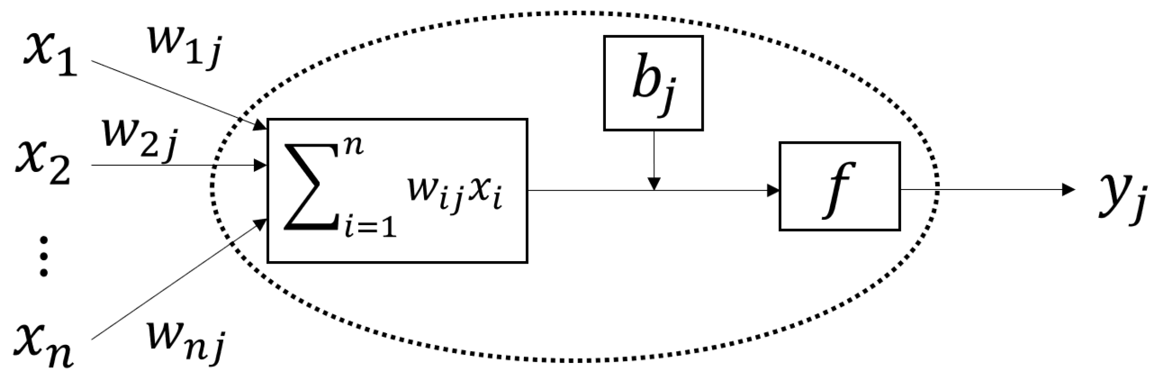
ANN process the information like the neural network of the human brain, i.e., by connecting different simple units/nodes, named as artificial neurons, to form different complex networks [19]. Each node includes an activation function to produce an output value based on one or multiple inputs. The output signal of a node can be passed to another node using a weighted connection. Thus, the output an ANN depends on the connection structure, the weight value and activation function [20]. A simple signal layer ANN is illustrated in Figure 1.

Given one unit (an artificial neuron) j, let its input signals connected from other units be x_i (i = 1, 2, …, n) with corresponding weights w_ij (i = 1, 2, …, n). There are two basic operations in the processing unit, namely summation and activation of the input signals [18]. The unit’s output of y_j is defined as:

$$y_j=f({\displaystyle {\sum }_{i=1}^n{w}_{ij}}{x}_i+t_j),$$

where t_j is a bias for the unit j, and f is the activation function which can be commonly defined as the sigmoid function [21]:

$$f(x)=\frac{1}{1+e^{-x}}.$$

The output y_j will pass to the connected units from the next layer as an input signal. Given a designed architecture, all units in ANNs are interconnected in different layers. A simple example of a three-layer ANN is shown in Figure 2: the information flows through the input, hidden and output layers. The input layer or the first layer contains the same number of units as the input vector size, followed by the hidden layer with an arbitrary number of units. The output layer aggregates the weighted outputs from the hidden layer units.

2.2. SVM

SVM is mainly based on the theory of statistical learning theory. It a machine learning tool for solving a convex quadratic problem containing linear constraints, in which local minimum does not exist. Linear support vector machines can be extended into nonlinear space by introducing the kernel method, which barely increases the computational cost for high-dimensional data. Vapnik and Chervonenkis proposed the VC theory of exponential function sets, which motivated the progress of support vector machines in the historical stage [22]. With the development and maturity of theoretical research, Boser et al. proposed SVM by harnessing the theory of statistical learning knowledge and realized the nonlinear support vector machine according to the kernel function theory [23]. With respect to the risk minimization principle, ANN employs the empirical mode while SVM relies on the structural mode. So far, it has been widely used in various classification tasks, such as pattern recognition, images and text classification. In addition, SVM has been used for the regression task with some loss functions [24].

SVM can realize the regression version, which is called support vector regression (SVR). SVR solves regression problems on the basis of support vector machines [25,26]. SVR has powerful learning ability and generalization ability suitable for a small set of samples and has got great success in forecasting work with promising results [27,28]. This results from that it can adaptively process various tasks through generalization and meanwhile gets gain access to satisfactory answers. In particular, a nonlinear relation can be transferred into a linear relation with the utilization of SVR and thus the task can be easily solved. A drawback is that this becomes time-consuming when the task scale becomes large [29,30].

For the decision function, it can be represented by:

$$f(x)=w^{T}x+b,$$

where w, x, and b represent the weight vector, the input vector, and the bias, respectively. For the training input vector and target output, we assume x_m and y_m be the m-th (m = 1, 2, …, M) input and output, respectively. Let C be a positive parameter for penalizing the samples which does not satisfy inequality constraints. The error function can be defined as:

$$J=\frac{1}{2}{w}^{T}w+C{\displaystyle {\sum }_{m=1}^M|y_m}-{f(x_m)|}_{\epsilon }.$$

The error function has two terms, which are used for penalizing model complexity and representing the ε-insensitive loss function, respectively. The loss function is mathematically given as:

$$|y_m-{f(x_m)|}_{\epsilon }=\max \left\{0,|y_m-f(x_m)|-\epsilon \right\}.$$

This function cannot penalize errors less than ε in order to reduce model complexity. The solution of minimizing the error function can be defined as:

$$f(x)={\displaystyle {\sum }_{m=1}^M({\alpha }_m^{\ast }-{\alpha }_m)}{x}_m^{T}x+b,$$

in which the parameters α_m and ${\alpha }_m^{*}$ are Lagrange multipliers. Support vectors from the training vectors give non-zero Lagrange multipliers and contribute directly to the solution, while the non-support vectors do not. The relationship between support vectors and the model complexity is that its number can measure the latter [31,32].

The key in SVR applications is the utilization of kernel functions, which can map non-linear data into spaces in which they are essentially linear for the optimization process. One can utilize the following kernel function:

$$K(x_m,x)=K(x_m^{T}x)=\varphi {(x_m)}^T\varphi (x).$$

Then, the model is changed into:

$$f(x)={\displaystyle {\sum }_{m=1}^M({\alpha }_m^{\ast }-{\alpha }_m)}K(x_m^{T}x)+b$$

For kernel functions, Gaussian, polynomial, and hyperbolic tangent type can be used. The Gaussian type is one of the most popular kernel functions used in empirical analysis, mathematically described as follows:

$$K(x_m,x)=\exp (-\gamma {\Vert x_m-x\Vert }^2), \mathrm{for} \gamma >0.$$

2.3. GBM

Friedman proposed the concept of gradient boosting and introduced the gradient boosting machine (GBM) technique for the extension of the boosting to the regression [33,34,35]. GBM has many applications in regression and classification by generating forecasting models in the form of the set of weak forecasting models (usually decision tree). GBM is a kind of boosting method. The basic idea of boosting is to utilize some way such that base learners of each round are more concerned about the misclassified learning samples of last round during the process of training, but GBM focuses on each modelling using the gradient descent direction in the previous model loss function. The negative gradient is used as the measurable indicator that base learners of last round and are fitted in the next round learning to correct mistakes appeared in the last round. The difference with traditional boosting is that the purpose of each computation is to reduce the residual of last computation. In order to eliminate the residual, one can refer to the gradient direction of residual decrease for model build-up. Thus, the building-up of each new model is to make the residual of the previous model cut down along the gradient direction in the gradient boosting, which greatly differs from traditional boosting in weighting correct and wrong samples.

GBM has been shown significant success deployed in various kinds of practical applications in different fields. It can be considered as a methodological framework, i.e., it is very flexible and customizable which can achieve high accuracy in many data mining tasks. However, in practice, the most issue of GBM is it memory-consumption. With respect to a GBM algorithm, given an output y, an input x, a training set ${\left\{\left(x_i,y_j\right)\right\}}_{i=1}^n$, and number of iterations M, we seek an approximation $\widehat{F}\left(x\right)$ for a function F(x) and the approximation requires minimizing the expected value of some specified loss function L(y, F(x)):

$$\widehat{F}\left(x\right)=\arg {\min }_F{{\rm E}}_{x,y}[L(y,F(x))]$$

The gradient boosting method assumes a real-valued y and seeks an approximation $\widehat{F}\left(x\right)$ and a base-learner model h_i(x):

$$\widehat{F}\left(x\right)={\displaystyle {\sum }_{i=1}^M{\rho }_i}{h}_i(x)+const.$$

$\widehat{F}\left(x\right)={\displaystyle {\sum }_{i=1}^M{\rho }_i}{h}_i(x)+const$ can be approximated in a greedy way:

$$F_0\left(x\right)=\arg {\min }_{\rho }{\displaystyle {\sum }_{i=1}^{N}L\left(y_i,\rho \right)},$$

$$F_m\left(x\right)=F_{m-1}\left(x\right)+\arg {\min }_{h_m}\left[{\displaystyle {\sum }_{i=1}^{N}L\left(y_i,F_{m-1}\left(x_i\right)+h_m\left(x_i\right)\right)}\right].$$

The negative gradient is calculated by:

$${\tilde{y}}_i=-{\left[\frac{\partial L\left(y_i,F\left(x_i\right)\right)}{\partial F\left(x_i\right)}\right]}_{F\left(x\right)=F_{m-1}\left(x\right)}, i=1,\cdots ,N.$$

$h_m(x)$ is utilized for fitting ${\tilde{y}}_i$ through minimizing the squared error:

$${\alpha }_m=\arg {\min }_{\alpha ,\beta }{\displaystyle {\sum }_{i=1}^N[{\tilde{y}}_i-\beta h\left(x_i;\alpha \right)}{]}^2$$

One can employ line search for ρ_m so as to minimize the loss function:

$${\rho }_m=\arg {\min }_{\rho }{\displaystyle {\sum }_{i=1}^{N}L\left(y_i,F_{m-1}\left(x_i\right)+\rho h\left(x_i;{\alpha }_m\right)\right)}.$$

Finally, it is updated:

$$F_m\left(x\right)=F_{m-1}\left(x\right)+{\rho }_{m}h\left(x;{\alpha }_m\right).$$

2.4. GPR

GPR builds upon the Gaussian process (GP). GP is a kind of random processes that generalizes multivariate normal distribution in the infinite dimensional space and therefore is defined in the distribution over functional values. It is a powerful nonlinear multivariate interpolation tool. The prior information of GP is used for the inference of continuous value, which is referred to as GPR. GPR is an interpolation method, in which the interpolation is controlled by prior covariances, and can give the best linear unbiased prediction for median under the appropriate prior assumptions. It can also be illustrated by the theory of Bayesian inference [36]. GPR is proposed by Rasmussen et al. at first, which is an efficient machine learning algorithm based on kernel function and provides a principle, practicable, and probabilistic method for kernel machine learning [37,38]. In comparison with other machine learning methods, the advantages of GPR lie in being able to seamlessly integrate multiple machine learning tasks such as parameter estimation; therefore, the regression can be obviously simplified and the objective influence for the result is slight, more convenient for an explanation. GPR possesses excellent performance with relatively small training dataset and offers confidence interval for prediction by adopting flexible kernel function. However, a known bottleneck is that the computation complexity in prediction is cubic about |x|, thus it is infeasible for large datasets.

Let X be the matrix of input vectors and x_i be the i-th training input vector. Let K(X, X) be the covariance matrix for pairwise vectors, such that:

$$K(x_i,x_j)={\sigma }_f^2{e}^{-\frac{\Vert x_i-{x_j\Vert }^2}{2{\gamma }^2}}.$$

The variable f follows the following distribution:

$$f-m_f(0,K(X,X)),$$

which is a multivariate Gaussian density distribution. m_f(μ, Σ) represents the normal density function. Additionally, some noise can be added for the estimation of target output y:

$$y=f+\epsilon ,$$

where the noise $\epsilon$ yields the independent normal distribution with mean zero and standard deviation σ_n. Then, given an input vector x_* from the test data, the output ${\widehat{f}}_{*}$ becomes:

$${\widehat{f}}_{\ast }=E(f_{\ast }|X,y,x_{\ast })=K(x_{\ast },X){[K(X,X)+{\sigma }_n^{2}I]}^{-1}y.$$

3. Data Preparation and Description

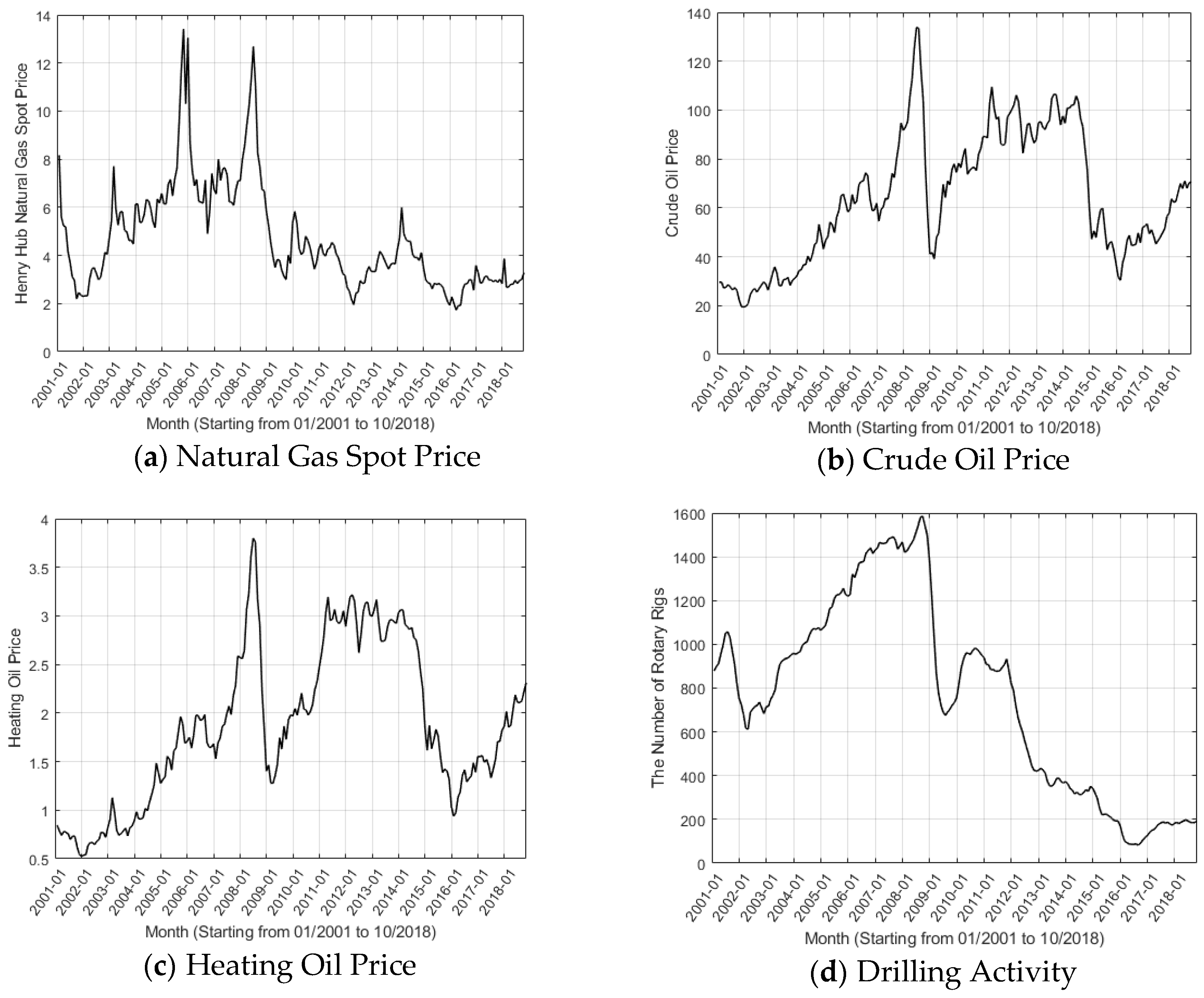
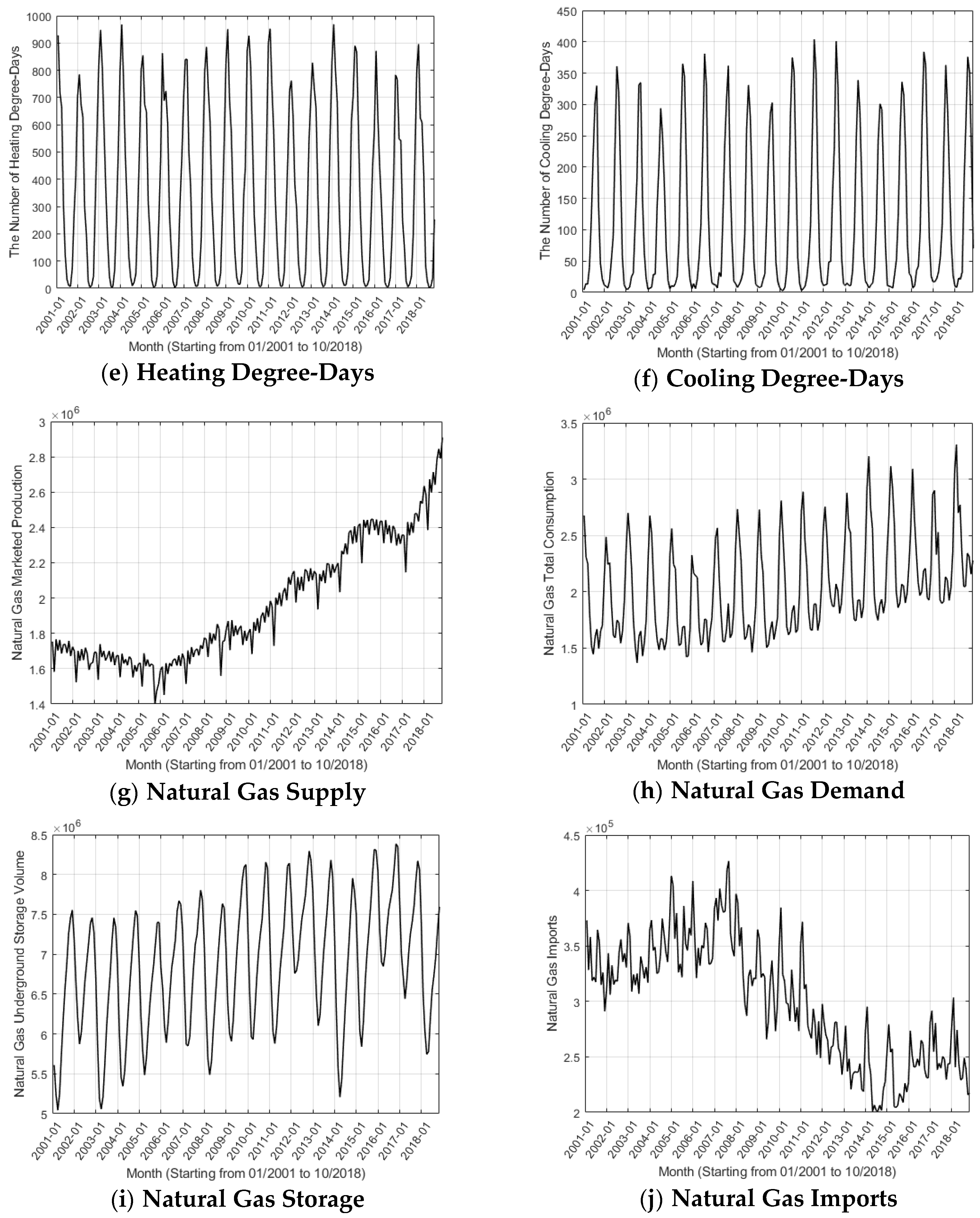
There exist a great number of factors that affect the natural gas price, e.g., crude oil, heating oil, drilling activity, temperature, natural gas supply, demand, storage, imports, etc. To better forecast the gas price, we should consider as many relevant factors as possible. To begin with, the relationship between crude oil price and natural gas price is a continuous research focus [39]. They often behave a strong connection and crude oil price fluctuations usually affect the natural gas price. Secondly, the natural gas can be seen as an alternative energy resource to heating oil in US industry and power plants, thus, their demands can be shifted between each other based on the market prices [40]. Thirdly, the prosperity level of the natural gas market can be reflected based on the gas drilling activities [41]. Fourthly, the price of natural gas often suffers from the temperature and weather changes are also a key factor [42]. The demand for natural gas varies with season. In addition, obviously, natural gas supply, demand, storage, and imports are important indicators related to natural gas price. Thus, the abovementioned variables include crude oil price (WTI), heating oil price (HO), natural gas rotary rigs (NGRR), heating degree-days (HDD), cooling degree-days (CDD), natural gas marketed production (NGMP), natural gas total consumption (NGTC), natural gas underground storage volume (NGUSV), and natural gas imports (NGI) are used as inputs in this study.

Table 1. A list of the variable used in this study.

Variables	Data	Unit	Source
Natural gas price	Henry Hub Natural Gas Spot Price	Dollars/million btu	EIA
Crude Oil Price	Cushing, OK WTI Spot Price FOB	Dollars/barrel	EIA
Heating Oil Price	New York Harbor No. 2 Heating Oil Spot Price FOB	Dollars/gallon	EIA
Drilling Activity	U.S. Natural Gas Rotary Rigs in Operation	Count	EIA
Temperature	Heating Degree-Days	Number	NOAA
	Cooling Degree-Days	Number
Natural Gas Supply	U.S. Natural Gas Marketed Production	Million Cubic Feet	EIA
Natural Gas Demand	U.S. Natural Gas Total Consumption	Million Cubic Feet	EIA
Natural Gas Storage	U.S. Total Natural Gas Underground Storage Volume	Million Cubic Feet	EIA
Natural Gas Imports	U.S. Natural Gas Imports	Million Cubic Feet	EIA

lists the details of several variables in terms of data, unit, and source, where EIA [43] and NOAA [44] represent the US Energy Information Administration National Oceanic and Atmospheric Administration, respectively.

Natural gas price is the output variable and Henry Hub Natural Gas Spot Price is adopted, which is from the US EIA [43] and quoted in dollars per million btu. Henry Hub is the earliest representative American natural gas spot trading centre and is also the largest one until now. It has greatly benefited the development of the natural gas market and energy economic prosperity since its establishment. For the abovementioned variables, our dataset comprises monthly data within the period from January 2001 to October 2018 and all data in the months in this period are complete, which guarantees the availability of data.

Historical trends of natural gas and relevant variables are described in Figure 3, in which Figure 3a depicts the natural Henry Hub spot price from January 2001 to October 2018, containing a total of 214 records. It can be known that during this period, the average natural price was $4.71, the median was $4.05, and the standard deviation was $2.22. As shown in Figure 3a, the peak price (13.42 dollars per million btu) and the bottom price (1.73 dollars per million btu) occurred in October 2005 and March 2006, respectively. One can easily find that there are a few sharp rises for natural gas before 2009. The first sharp rise appeared in the winter of 2003, which is mainly caused by extremely cold weather, consistent with the case of storage reserves being substantially reduced, as shown in Figure 3i. The second upsurge appeared in October to December of 2005 when hurricanes Katrina and Rita happened in succession. Hurricanes make natural gas supply drop markedly. The lowest marketed production is in September 2005, only 1,400,941 million cubic feet, while in October, it increased by 74,708 million cubic feet, which can be observed in Figure 3g. The third rapid rise is before the global financial crisis in 2008, which, to a great extent, was caused by an increase of the crude oil prices that led a strong demand for natural gas, as shown in Figure 3b–d. Since 2009, natural gas in the US has remained at a low level and this is mainly due to two aspects: one is that the demand for natural gas is not urgent. The other aspect is the oversupply due to the rapid development of shale gas.

Comparing Figure 3a–c can find the natural gas price, WTI price, and HO price have similar trends before 2009. After 2009, the WTI price and HO price behaviour show a basically consistent trend. As for the number of rotary rigs, it shows a similar tendency as natural gas price according to the comparison between Figure 3a and Figure 3d. The relationships between natural gas price and the number of rotary rigs is quite telling, as it shows that business activities in the drilling industry depend on market conditions and potential value to a great extent.

The fluctuation range of HDD doubles that of CDD or so and thereby the uncertainty of temperature changes in winter is greater than that in autumn in the US, affecting the expectation of natural gas demand in winter. It can be seen from Figure 3g,i that the supply of natural gas basically went up and the storage volume increased continually during the observation period, which results from the shale gas revolution in the US. Total consumption of natural gas has a rising trend while the imports show the opposite.

Table 2. Summary statistics of natural gas prices and relevant variables.

Variables	Max	Min	Median	Mean	SD	RSD
NGSP	13.42	1.73	4.045	4.7064	2.2156	0.4708
WTI	133.8	19.39	61.795	63.8696	26.5254	0.41538
HO	3.801	0.524	1.7695	1.8602	0.806	0.4333
NGRR	1585	82	792.5	762.1682	445.8986	0.5850
HDD	969	3	279.5	352.5374	313.4179	0.8890
CDD	404	3	52.5	115.9766	122.9591	1.0602
NGMP	2,909,415	1,400,941	1,827,382	1,959,300	340,660	0.1739
NGTC	3,307,711	1,368,369	1,926,900	2,036,900	424,400	0.2084
NGUSV	8,384,087	5,041,971	6,920,016	6,865,600	806,420	0.1175
NGI	426,534	200,669	306,952	300,010	55,160	0.1839

lists the descriptive statistics for natural gas spot price (NGSP)and relevant variables including max, min, median, mean, standard deviation (SD), and relative standard deviation (RSD). It can be seen from Table 2 that we can know that the standard deviation of natural gas price is far smaller than that of other variables, except for heating oil price, while the relative standard deviation of natural gas is at the mid-level among all the variables.

Table 3. Correlations between variables.

Variables	NGSP	WTI	HO	NGRR	HDD	CDD	NGMP	NGTC	NGUSV	NGI
NGSP	1.0000
WTI	0.1964	1.0000
HO	0.1321	0.9805	1.0000
NGRR	0.7504	0.0936	0.0144	1.0000
HDD	0.0911	−0.0860	−0.0493	0.0221	1.0000
CDD	−0.0590	0.0897	0.0592	−0.0299	−0.8244	1.0000
NGMP	−0.6053	0.1976	0.2814	−0.8315	−0.0872	0.1117	1.0000
NGTC	−0.2021	0.0238	0.0958	−0.3744	0.8085	−0.4791	0.3956	1.0000
NGUSV	−0.3099	0.1341	0.1618	−0.2203	−0.2975	0.2449	0.2933	−0.1730	1.0000
NGI	0.6082	−0.2653	−0.3319	0.8078	0.2445	−0.0989	−0.8007	−0.0906	−0.2951	1.0000

shows the correlations among the variables. It can be known from Table 3 that with respect to the correlation between the natural gas price and other variables [45], the strongest is with the number of rotary rigs and second are marketed production and imports. The weakest correlations are with heating degree-days and cooling degree-days. Among relevant variables, the crude oil price and the heating oil price have the strongest correlation. The variables with strong correlations also occur between the number of rotary rigs and marketed production, the number of rotary rigs and imports, heating degree-days and cooling degree-days, heating degree-days and total consumption, and marketed production and imports. The variables with weak correlations occur between crude oil price and total consumption, the number of rotary rigs and heating degree-days, and the number of rotary rigs and cooling degree-days, in which the weakest correlation is between the number of rotary rigs and heating oil price.

4. Empirical Study

4.1. Forecasting Performance Evaluation Criteria

There existed many model evaluation criteria and we choose some classic statistical criteria for testing model forecasting performance. R-square (R²) is often used for measuring the goodness-of-fit [46]

$$R-square(R^2)=\left[1-\frac{\frac{1}{N}{\displaystyle {\sum }_{t=1}^N{\left({\tilde{y}}_t-y_t\right)}^2}}{\mathrm{var}\left(y\right)}\right],$$

where y_t and ${\tilde{y}}_t$ represent the actual value and the prediction value at the time t, respectively. N means the total number of samples in the dataset. R² can manifest the goodness and badness of fitting by using changes in the data. The value of R² ranges from is from zero to one. The regression fitting effect becomes better when the value of R² is closer to 1 [47,48]. In general, the value greater than 0.8 can indicate that the model has a high enough goodness-of-fit. Moreover, there are four criteria used for measuring the forecasting errors.

Mean absolute error (MAE) is also a common forecasting performance evaluation tool obtained by averaging the absolute errors [49,50]:

$$MAE=\frac{1}{N}\times {\displaystyle {\sum }_{t=1}^N\left|{\tilde{y}}_t-y_t\right|}.$$

Mean square error (MSE) is an average of the quadratic sum of the deviation of forecasting value and actual value and is good at measuring the degree of change [51,52]. The prediction model gets better accuracy with the decrease of the MSE value. In contrast to MAE, MSE enlarges the value of great prediction deviation and compares the stability of different prediction models. It is represented as:

$$MSE=\frac{1}{N}\times {{\displaystyle {\sum }_{t=1}^N\left({\tilde{y}}_t-y_t\right)}}^2.$$

Root-mean-square error (RMSE) can be directly obtained from MSE by calculating the square root [53,54]. It is very sensitive to the very large or very small error value and thus has a good reflection for precision, formulated as:

$$RMSE=\sqrt{MSE}=\sqrt{\frac{1}{N}\times {{\displaystyle {\sum }_{t=1}^N\left({\tilde{y}}_t-y_t\right)}}^2}.$$

Mean absolute percentage error (MAPE) is often used as a loss function, since it can intuitively explain the relative errors [55,56]. It considers not only the deviation of prediction value and actual value, but also the ratio between them. It is given by:

$$MAPE=\frac{1}{N}\times {\displaystyle {\sum }_{t=1}^N\left|\frac{{\tilde{y}}_t-y_t}{y_t}\right|}.$$

In the above-mentioned evaluation indices including MAE, MSE, RMSE, and MAPE, the smaller the value, the better the forecasting model accuracy.

4.2. Model Validation Technique

Cross-validation is an important method for model selection to obtain feasible and stable models in machine learning. In cross-validation, K-fold validation is a common method of preventing over-fitting when the model is too complex. It has been demonstrated that compared with Holdout method and Leave-one-out cross-validation, K-fold validation has more advantages in precision estimation and model selection [57]. With the help of K-fold validation, we partition training dataset into K equal folds, of which K − 1 folds are employed for model training while the remaining fold is used for validation. This operation of training and validation is repeatedly done by rotating K folds. After carrying out this operation K times, we gather all the errors to calculate out the final error. Note that, K is often taken as 10 in reality [57].

4.3. Model Parameter Selection

Machine learning methods involve many parameters, some of which are key parameters and thus are carefully selected. The complexity of the model is often related to these key parameters, which is also called model selection parameters. With regard to ANN, we choose a nonlinear autoregressive model with external input. The number of hidden neurons and the number of delays are selected as 10 and 2, respectively. In the train network, the training algorithm chosen is Levenberg-Marquardt, which typically needs more memory but less time. According to the MSE value of the validation samples, the training will stop automatically once the generalization cannot improve.

The kernel function should be carefully selected in the SVM model. In order to pick off the appropriate kernel function, our strategy is to test different functions and then the one with minimum error is what we need. Accordingly, six common kernel functions including linear type, quadratic type, cubic type, fine Gaussian, medium Gaussian, and coarse Gaussian are investigated, as shown in

Table 4. RMSE values of different kernel functions.

Kernel Function	1	2	3	4	5		96	97	98	99	100
Linear	1.4296	1.4284	1.4245	1.4373	1.4175	……	1.4200	1.4262	1.4246	1.4347	1.4175
Quadratic	1.0052	1.0185	1.0037	1.0274	0.9923	……	1.0067	1.0153	1.0056	0.9848	1.0319
Cubic	0.8373	0.8401	0.8187	0.9027	0.8367	……	0.8322	0.8853	0.9418	0.8103	0.8505
Fine Gaussian	1.8277	1.8442	1.8259	1.8393	1.8154	……	1.8336	1.8347	1.8400	1.8535	1.8437
Medium Gaussian	1.0947	1.0996	1.0761	1.1129	1.0653	……	1.0851	1.0943	1.0947	1.0731	1.1001
Coarse Gaussian	1.4394	1.4425	1.4318	1.4414	1.4256	……	1.4292	1.4283	1.4320	1.4363	1.4261

. Over one hundred experiments are deduced to the cubic type, which has better results than others overall and thereby serves as the kernel function of SVM in this study.

GBM requires a reasonable loss function. The gradient boosting strategy harnesses several popular loss criteria: least-squares, least absolute deviation, Huber, logistic binomial log-likelihood, etc. We choose least-squares as loss function, since only the case of least-squares is suitable for regression model while others are usually applied in classification. In addition, the covariance function or kernel function is needed in GPR, such as Gaussian kernel and squared exponential kernel used in many machine learning algorithms. In this paper, squared exponential is used as the kernel function, since it behaves better results.

4.4. Empirical Study Results

Based on the before-mentioned machine learning methods, prepared data, forecasting performance evaluation criteria, model validation technique, and selected model parameters, the empirical study is carried out.

Table 5. Forecasting performance of four machine learning methods.

Model	R-Square	MAE	MSE	RMSE	MAPE
ANN	0.8904	0.5115	0.5363	0.7247	0.1117
SVM	0.8437	0.5673	0.7673	0.8757	0.1202
GBM	0.8006	0.6490	0.9786	0.9888	0.1366
GPR	0.8374	0.6026	0.7980	0.8932	0.1270

lists the data that describe the forecasting performance of four machine learning methods, in which each value is the average of one hundred tests for the purpose of more accurate results. Observing data of four criteria can easily find that the forecasting performance of ANN and SVM is better than that of GBM and GPR. In particular, ANN is obviously superior to other methods while GBM has the worst behaviour. Overall, the performance ranking is ANN, SVM, GPR, and GBM from strong to weak.

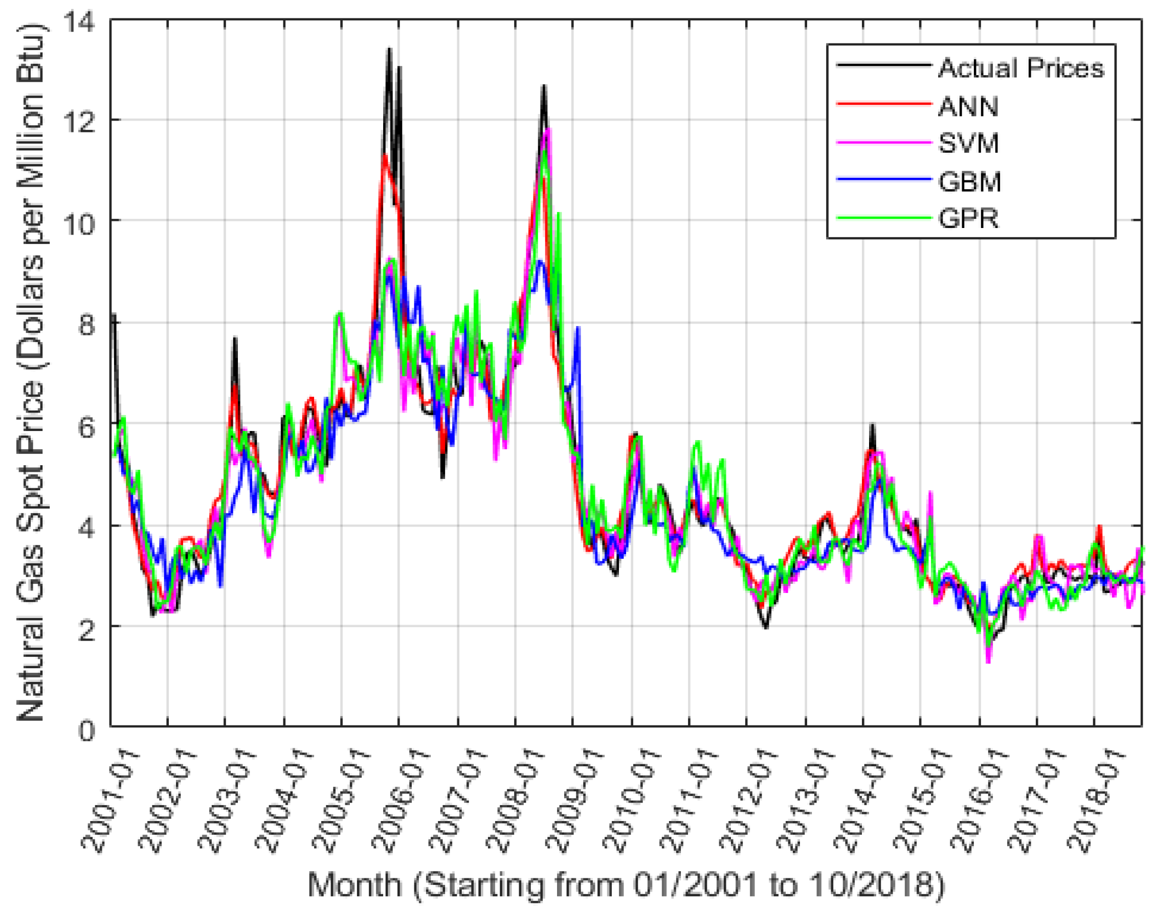
Figure 4 intuitively compares the prediction suitcases of four machine learning methods, which contains 214 observed values from January 2001 to October 2018. ANN delays two values, i.e., from March 2001. It can be obtained from Figure 4 that overall, all the methods have a strong prediction ability, since their predicted natural gas spot prices are close to the actual prices and approximatively depict the characteristics of the Henry Hub natural gas spot price time series. From the view of the whole tendency, ANN outperforms others, in particular, for the prediction of abnormal values at the beginning of 2009 and the second half of 2010. SVM and GPR are inferior to ANN, but SVM excels the other three methods in terms of price prediction in the middle of 2008. GBM behaves the worst prediction ability among the methods, especially for outliers.

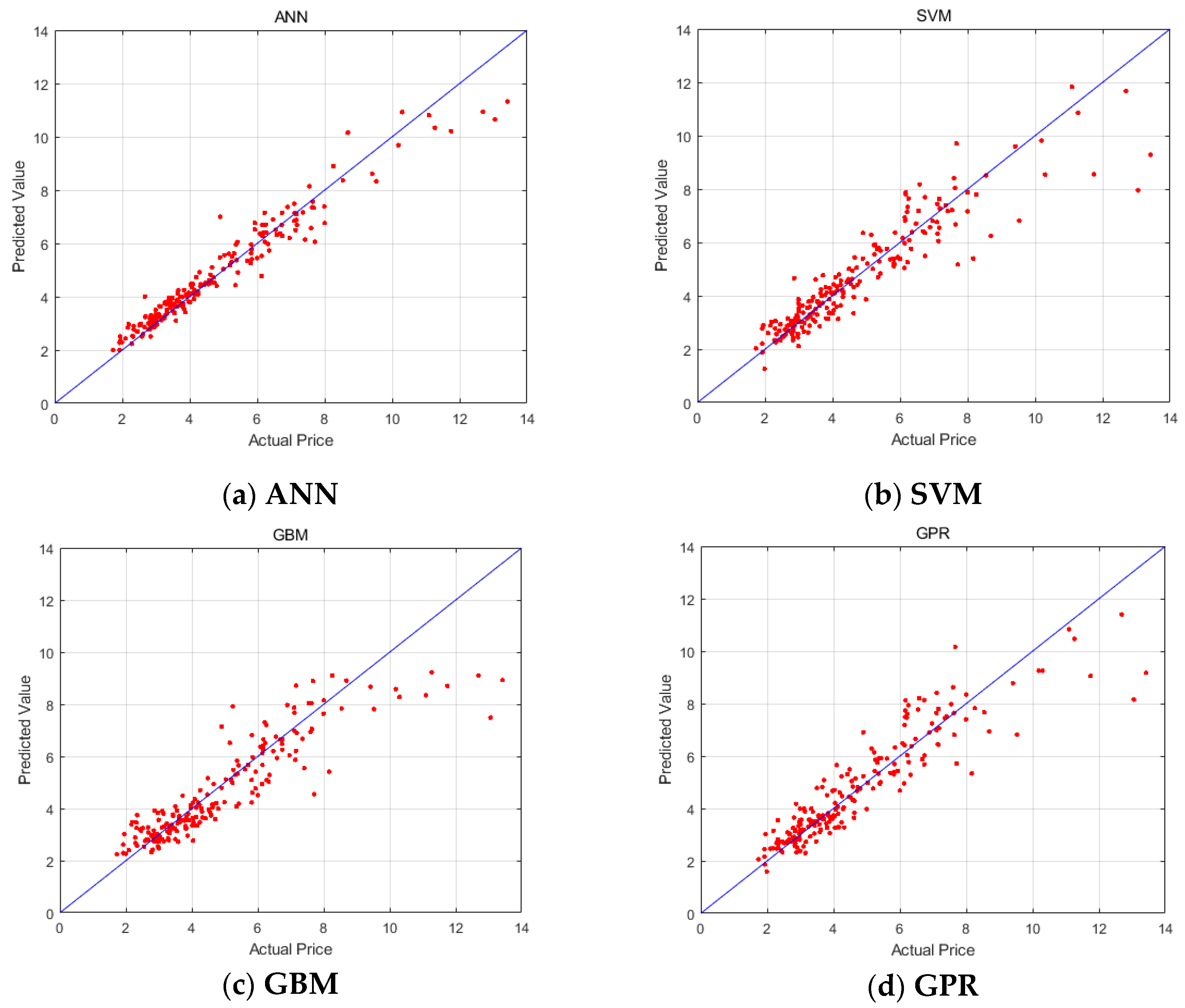
Figure 5 shows the distribution suitcases between predictive values and actual values. It can be seen that the actual normal price is centered around 2 to 8 and these four methods give a good prediction for normal values. The fluctuation of ANN is less than that of others. However, they are unsatisfactory when the price goes up greater than 8, e.g., from September to December and April to July 2008. The prediction of abnormal values is still a difficult task so far.

From the above results, we can understand that there are obviously distinct differences among the four machine learning models, and there is a general ranking reference. Overall, ANN and SVM have better prediction performance than GBM and GPR, where ANN wins the best and GBM is the worst. ANN has a good ability of self-learning, self-adapting, and self-organizing [58], which can analyze the patterns and rules of observed data and form complex non-linear functions through training, and adapt to large-scale, multi-factor, incomplete, and inaccurate data processing. The number of delays in ANN is 10 in this study, which is greater than traditional ANN’s (the number of delays is 3 at most). That may be one reason that ANN is superior to SVM. SVM has an abundant and theoretical foundation and has strong approximation ability and generalization ability based on structural risk minimization. SVM aims at small sample, of which the optimal solution is based on limited sample. GPR has a simplified regression process and easily explains the consequence. It has favourable performance in number and stability, but it is suitable for research on relatively small training dataset. GBM has a relatively weaker performance than the above methods in forecasting natural gas prices, however, we can obtain the degree of importance of explanatory variables by using GBM.

5. Conclusions

The aim of this study is to investigate natural gas price forecasting based on four machine learning methods (ANN, SVM, GBM, and GPR). Monthly Henry Hub natural gas spot price data from January 2001 to October 2018 (there are 215 observations) were used in four prediction methods. Nine variables were investigated as inputs, which are NGSP, WTI, HO, NGRR, HDD, CDD, NGMP, NGTC, NGUSV, and NGI. The method cross-validation was used in model training. Four forecasting performance evaluation criteria including R², MSE, RMSE, and MAPE are employed in prediction methods. Finally, the empirical results demonstrate that four prediction methods have decent performance in forecasting natural gas price. Overall, ANN and SVM have better forecasting performance than GBM and GPR. In particular, ANN obviously outperforms the other methods while GBM is the worst. This study could be improved by more thorough research, e.g., by comparing more different aspects of the prediction performance such as computation efficiency and using more diverse machine learning methods such as random forest [59,60]. For future work, we will evaluate the effect of emerging machine learning algorithms, such as deep learning and reinforcement learning, on energy price and correlation prediction.

References

- International Energy Agency (IEA). Key World Energy Statistics 2018. Available online: https://webstore.iea.org/key-world-energy-statistics-2018 (accessed on 30 April 2019).
- Afgan, N.H.; Pilavachi, P.A.; Carvalho, M.G. Multi-criteria evaluation of natural gas resources. Energy Policy 2007, 35, 704–713. [Google Scholar] [CrossRef]
- Abrishami, H.; Varahrami, V. Different methods for gas price forecasting. Cuad. Econ. 2011, 34, 137–144. [Google Scholar] [CrossRef] [Green Version]
- Busse, S.; Helmholz, P.; Weinmann, M. Forecasting day ahead spot price movements of natural gas—An analysis of potential influence factors on basis of a NARX neural network. In Proceedings of the Tagungsband der Multikonferenz Wirtschaftsinformatik (MKWI), Braunschweig, Germany; Available online: https://publikationsserver.tu-braunschweig.de/servlets/MCRFileNodeServlet/dbbs_derivate_00027726/Beitrag299.pdf (accessed on 30 April 2019).
- Azadeh, A.; Sheikhalishahi, M.; Shahmiri, S. A Hybrid Neuro-Fuzzy Approach for Improvement of Natural Gas Price Forecasting in Vague and Noisy Environments: Domestic and Industrial Sectors. In Proceedings of the International Conference on Trends in Industrial and Mechanical Engineering (ICTIME’2012), Dubai, United Arab Emirates, 24–25 March 2012. [Google Scholar]
- Salehnia, N.; Falahi, M.A.; Seifi, A.; Adeli, M.H.M. Forecasting natural gas spot prices with nonlinear modeling using gamma test analysis. J. Nat. Gas Sci. Eng. 2013, 14, 238–249. [Google Scholar] [CrossRef]
- Čeperić, E.; Žiković, S.; Čeperić, V. Short-term forecasting of natural gas prices using machine learning and feature selection algorithms. Energy 2017, 140, 893–900. [Google Scholar] [CrossRef]
- Su, M.; Zhang, Z.; Zhu, Y.; Zha, D. Data-Driven Natural Gas Spot Price Forecasting with Least Squares Regression Boosting Algorithm. Energies 2019, 12, 1094. [Google Scholar] [CrossRef]
- Lloyd, J.R. GEFCom2012 hierarchical load forecasting: Gradient boosting machines and Gaussian processes. Int. J. Forecast. 2014, 30, 369–374. [Google Scholar] [CrossRef] [Green Version]
- Cossock, D.; Zhang, T. Statistical Analysis of Bayes Optimal Subset Ranking. IEEE Trans. Inf. Theory 2008, 54, 5140–5154. [Google Scholar] [CrossRef] [Green Version]
- Landry, M.; Erlinger, T.P.; Patschke, D.; Varrichio, C. Probabilistic gradient boosting machines for GEFCom2014 wind forecasting. Int. J. Forecast. 2016, 32, 1061–1066. [Google Scholar] [CrossRef]
- Zhang, Y.; Haghani, A. A gradient boosting method to improve travel time prediction. Transp. Res. Part C Emerg. Technol. 2015, 58 Pt B, 308–324. [Google Scholar] [CrossRef]
- Candanedo, L.M.; Feldheim, V.; Deramaix, D. Data driven prediction models of energy use of appliances in a low-energy house. Energy Build. 2017, 140, 81–97. [Google Scholar] [CrossRef]
- Deng, X.; Han, J.; Yin, F. Net Energy, CO2 Emission and Land-Based Cost-Benefit Analyses of Jatropha Biodiesel: A Case Study of the Panzhihua Region of Sichuan Province in China. Energies 2012, 5, 2150–2164. [Google Scholar] [CrossRef]
- Sun, A.Y.; Wang, D.; Xu, X. Monthly streamflow forecasting using Gaussian Process Regression. J. Hydrol. 2014, 511, 72–81. [Google Scholar] [CrossRef]
- Yu, J.; Chen, K.; Mori, J.; Rashid, M.M. A Gaussian mixture copula model based localized Gaussian process regression approach for long-term wind speed prediction. Energy 2013, 61, 673–686. [Google Scholar] [CrossRef]
- Salcedo-Sanz, S.; Casanova-Mateo, C.; Muñoz-Marí, J.; Camps-Valls, G. Prediction of Daily Global Solar Irradiation Using Temporal Gaussian Processes. IEEE Geosci. Remote Sens. Lett. 2014, 11, 1936–1940. [Google Scholar] [CrossRef]
- McCulloch, W.S.; Pitts, W. A Logical Calculus of Ideas Immanent in Nervous Activity. Bull. Math. Biophys. 1943, 5, 115–133. [Google Scholar] [CrossRef]
- Kurbatsky, V.G.; Sidorov, D.N.; Spiryaev, V.A.; Tomin, N.V. Forecasting nonstationary time series based on Hilbert-Huang transform and machine learning. Autom. Remote Control 2014, 75, 922–934. [Google Scholar] [CrossRef]
- Maier, H.R.; Dandy, G.C. Neural networks for the prediction and forecasting of water resources variables: A review of modelling issues and applications. Environ. Model. Softw. 2000, 15, 101–124. [Google Scholar] [CrossRef]
- Magoules, F.; Zhao, H.X. Data Mining and Machine Learning in Building Energy Analysis; ISTE Ltd. and John Wiley & Sons, Inc.: Hoboken, NJ, USA, 2016. [Google Scholar]
- Vapnik, V.N.; Chervonenkis, A.Y. On the uniform convergence of relative frequencies of event to their probabilities. Sov. Math. Dokl. 1968, 9, 915–918. [Google Scholar]
- Boser, B.E.; Guyon, I.M.; Vapnik, V.N. A training algorithm for optimal margin classifiers. In Proceedings of the 5th Annual Workshop on Computational Learning Theory, Pittsburgh, PA, USA, 27–29 July 1992; ACM Press: New York, NY, USA, 1992; pp. 144–152. [Google Scholar] [Green Version]
- Vapnik, V.N. Statistical Learning Theory; Wiley: New York, NY, USA, 1998. [Google Scholar]
- Zhang, W.Y.; Hong, W.C.; Dong, Y.; Tsai, G.; Sung, J.T.; Fan, G.F. Application of SVR with chaotic GASA algorithm in cyclic electric load forecasting. Energy 2012, 45, 850–858. [Google Scholar] [CrossRef]
- Lauret, P.; Voyant, C.; Soubdhan, T.; David, M.; Poggi, P. A benchmarking of machine learning techniques for solar radiation forecasting in an insular context. Sol. Energy 2015, 112, 446–457. [Google Scholar] [CrossRef]
- Taghavifar, H.; Mardani, A. A comparative trend in forecasting ability of artificial neural networks and regressive support vector machine methodologies for energy dissipation modeling of off-road vehicles. Energy 2014, 66, 569–576. [Google Scholar] [CrossRef]
- Hong, W.C. Load forecasting by seasonal recurrent SVR (support vector regression) with chaotic artificial bee colony algorithm. Energy 2011, 36, 5568–5578. [Google Scholar] [CrossRef]
- Zhao, H.X.; Magoulès, F. Parallel support vector machines applied to the prediction of multiple buildings energy consumption. J. Algorithms Comput. Technol. 2010, 4, 231–250. [Google Scholar] [CrossRef]
- Cherkassky, V.; Ma, Y. Practical selection of SVM parameters and noise estimation for SVM regression. Neural Netw. 2004, 17, 113–126. [Google Scholar] [CrossRef] [Green Version]
- Chalimourda, A.; Scholkopf, B.; Smola, A.J. Experimentally optimal in support vector regression for different noise models and parameter settings. Neural Netw. 2004, 17, 127–141. [Google Scholar] [CrossRef]
- Li, Q.; Meng, Q.; Cai, J.; Yoshino, H.; Mochida, A. Predicting hourly cooling load in the building: A comparison of support vector machine and different artificial neural networks. Energy Convers. Manag. 2009, 50, 90–96. [Google Scholar] [CrossRef]
- Freund, Y.; Schapire, R.E. A Decision-Theoretic Generalization of On-Line Learning and an Application to Boosting. J. Comput. Syst. Sci. 1997, 55, 119–139. [Google Scholar] [CrossRef] [Green Version]
- Friedman, J.; Hastie, T.; Tibshirani, R. Additive logistic regression: A statistical view of boosting (With discussion and a rejoinder by the authors). Ann. Stat. 2000, 28, 337–407. [Google Scholar] [CrossRef]
- Friedman, J.H. Greedy Function Approximation: A Gradient Boosting Machine. Ann. Stat. 2001, 29, 1189–1232. [Google Scholar] [CrossRef]
- Williams, C.K.I. Prediction with Gaussian processes: From linear regression to linear prediction and beyond. In Learning in Graphical Models; Springer: Dordrecht, The Netherlands, 1998; pp. 599–621. [Google Scholar]
- Williams, C.K.I.; Rasmussen, C.E. Gaussian processes for regression. Adv. Neural Inf. 1996, 514–520. Available online: http://publications.eng.cam.ac.uk/330944/ (accessed on 30 April 2019).
- Rasmussen, C.E.; Williams, C.K.I. Gaussian Processes for Machine Learning; MIT Press: Cambridge, MA, USA, 2006. [Google Scholar]
- Shi, X.; Variam, H.M.P. East Asia’s gas-market failure and distinctive economics—A case study of low oil prices. Appl. Energy 2017, 195, 800–809. [Google Scholar] [CrossRef]
- Ohana, S. Modeling global and local dependence in a pair of commodity forward curves with an application to the US natural gas and heating oil markets. Energy Econ. 2010, 32, 373–388. [Google Scholar] [CrossRef]
- Ji, Q.; Zhang, H.-Y.; Geng, J.-B. What drives natural gas prices in the United States?—A directed acyclic graph approach. Energy Econ. 2018, 69, 79–88. [Google Scholar] [CrossRef]
- Geng, J.-B.; Ji, Q.; Fan, Y. The behaviour mechanism analysis of regional natural gas prices: A multi-scale perspective. Energy 2016, 101, 266–277. [Google Scholar] [CrossRef]
- EIA. Available online: https://www.eia.gov/ (accessed on 25 March 2019).
- NOAA. Available online: https://www.noaa.gov/ (accessed on 25 March 2019).
- Liu, F.; Li, R.; Li, Y.; Cao, Y.; Panasetsky, D.; Sidorov, D. Short-term wind power forecasting based on T-S fuzzy model. In Proceedings of the 2016 IEEE PES Asia-Pacific Power and Energy Engineering Conference (APPEEC), Xi’an, China, 25–28 October 2016; pp. 414–418. [Google Scholar]
- Cameron, A.C.; Windmeijer, F.A. An r-squared measure of goodness of fit for some common nonlinear regression models. J. Econ. 1997, 77, 329–342. [Google Scholar] [CrossRef]
- Jin, R.; Chen, W.; Simpson, T.W. Comparative studies of metamodelling techniques under multiple modelling criteria. Struct. Multidiscipl. Optim. 2001, 23, 1–13. [Google Scholar] [CrossRef]
- Touzani, S.; Granderson, J.; Fernandes, S. Gradient boosting machine for modeling the energy consumption of commercial buildings. Energy Build. 2018, 158, 1533–1543. [Google Scholar] [CrossRef] [Green Version]
- Willmott, C.J.; Matsuura, K. Advantages of the mean absolute error (MAE) over the root mean square error (RMSE) in assessing average model performance. Clim. Res. 2005, 30, 79–82. [Google Scholar] [CrossRef] [Green Version]
- Chai, T.; Draxler, R.R. Root mean square error (RMSE) or mean absolute error (MAE)?—Arguments against avoiding RMSE in the literature. Geosci. Model Dev. 2014, 7, 1247–1250. [Google Scholar] [CrossRef]
- Willmott, C.J. Some comments on the evaluation of model performance. Bull. Am. Meteorol. Soc. 1982, 63, 1309–1313. [Google Scholar] [CrossRef]
- Hyndman, R.J.; Koehler, A.B. Another look at measures of forecast accuracy. Int. J. Forecast. 2006, 22, 679–688. [Google Scholar] [CrossRef] [Green Version]
- Willmott, C.J. On the validation of models. Phys. Geogr. 1981, 2, 184–194. [Google Scholar] [CrossRef]
- Voyant, C.; Notton, G.; Kalogirou, S.; Nivet, M.L.; Paoli, C.; Motte, F.; Fouilloy, A. Machine learning methods for solar radiation forecasting: A review. Renew. Energy 2017, 105, 569–582. [Google Scholar] [CrossRef]
- De Myttenaere, A.; Golden, B.; le Grand, B.; Rossic, F. Mean Absolute Percentage Error for regression models. Neurocomputing 2016, 192, 38–48. [Google Scholar] [CrossRef] [Green Version]
- Kim, S.; Kim, H. A new metric of absolute percentage error for intermittent demand forecasts. Int. J. Forecast. 2016, 32, 669–679. [Google Scholar] [CrossRef] [Green Version]
- Kohavi, R. A study of cross-validation and bootstrap for accuracy estimation and model selection. In Proceedings of the 14th International Joint Conference on Artificial Intelligence (IJCAI), Montreal, QC, Canada, 20–25 August 1995; pp. 1137–1145. [Google Scholar]
- Kurbatsky, V.G.; Sidorov, D.N.; Spiryaev, V.A.; Tomin, N.V. The hybrid model based on Hilbert-Huang Transform and neural networks for forecasting of short-term operation conditions of power system. In Proceedings of the 2011 IEEE Trondheim PowerTech, Trondheim, Norway, 19–23 June 2011; pp. 1–7. [Google Scholar]
- Khaidem, L.; Saha, S.; Dey, S.R. Predicting the direction of stock market prices using random forest. arXiv 2016, arXiv:1605.00003. [Google Scholar]
- Zhukov, A.V.; Sidorov, D.N.; Foley, A.M. Random forest based approach for concept drift handling. In Proceedings of the International Conference on Analysis of Images, Social Networks and Texts, Yekaterinburg, Russia, 7–9 April 2016; pp. 69–77. [Google Scholar]
Figure 1.
A single artificial neuron process.
Figure 2.
Feed-forward ANNs.