Global Solar Radiation Prediction Using Hybrid Online Sequential Extreme Learning Machine Model

Abstract

Accurate global solar radiation prediction is highly essential for related research on renewable energy sources. The cost implication and measurement expertise of global solar radiation emphasize that intelligence prediction models need to be applied. On the basis of long-term measured daily solar radiation data, this study uses a novel regularized online sequential extreme learning machine, integrated with variable forgetting factor (FOS-ELM), to predict global solar radiation at Bur Dedougou, in the Burkina Faso region. Bayesian Information Criterion (BIC) is applied to build the seven input combinations based on speed (W_speed), maximum and minimum temperature (T_max and T_min), maximum and minimum humidity (H_max and H_min), evaporation (E_o) and vapor pressure deficiency (V_PD). For the difference input parameters magnitudes, seven models were developed and evaluated for the optimal input combination. Various statistical indicators were computed for the prediction accuracy examination. The experimental results of the applied FOS-ELM model demonstrated a reliable prediction accuracy against the classical extreme learning machine (ELM) model for daily global solar radiation simulation. In fact, compared to classical ELM, the FOS-ELM model reported an enhancement in the root mean square error (RMSE) and mean absolute error (MAE) by (68.8–79.8%). In summary, the results clearly confirm the effectiveness of the FOS-ELM model, owing to the fixed internal tuning parameters.

1. Introduction

Over the past five decades, research has revealed the need and necessity for adequate energy harvesting for multiple purposes including economic, social, and cultural development. Meanwhile, the UN general assembly’s announcement of the right to public, individual, and non-governmental organizational development in 1986 climaxed this passion. This declaration marked the beginning of the universal and inalienable equality of the human right to access to food, housing, employment, income, and education. This is concluded in the universal openness to all-round development [1]. Every activity directly linked to the realization of the human development agenda is energy-driven. Moreover, several studies have investigated the relationship of the energy level of several countries to their levels of development [2]. Consequently, the findings of these studies have reported a positive relationship of energy utilization with living standards. The level of energy usage in the developed nations is lower. Advanced countries are significantly consuming the energy, which greatly affects the levels of development in backward and developing countries [3].

Since energy is the main factor that drives all developmental processes, its effect on human, crops, plants, animals, and ecosystems depends on the form of energy employed [4,5]. Studies have reported two forms of available energy on Earth (renewable and non-renewable energies) [6]. The method employed in harnessing and applying these forms of energy for human use is very important in the way they affect humankind and the immediate environment. The uncontrolled utilization of the nonrenewable form of energy has been linked to several factors such as climate change, global warming, environmental pollution, and other economic and environmental hazards. Similarly, the renewable form of energy, which is globally available at varying levels, ought to be given attention. This form of energy can be obtained from natural processes, and therefore posits minimal or zero impact on humans and their immediate environment.

Renewable energy sources have attracted much research interest in the 21st century due to the discoveries of the impact of non-renewable energy on the environment. This interest is because renewable energy is sustained by natural processes, which contribute nothing to the generation of GHGs, global warming and climate change [7]. Since the discovery of solar radiation as a renewable energy source in the mid-19th century become important due to its availability, it has received global attention as it can match the power-generating capacity of fossil fuels.

The emerging climate challenges are having a serious effect on the Sub-Saharan region of Africa, as the two hydropower plants which generate 22 MW and the small-scale plant that generate 3 MW with a mean production of 80 GWh (60 130 GWhyr⁻¹) depend on rainfall, which is continuously decreasing [8]. However, wind energy is least attractive in Burkina Faso due to the low wind speed experienced in the country. Thus, Burkina Faso is left with solar as its main source of energy so as to reduce the importation of fossil fuel electricity from its neighboring countries, and enhance the 0.1% total solar energy utilization capacity recorded in 2014 [9].

The solar radiation process is complex in nature, where several other climatological and atmospheric elements such as wind speed, evaporation, humidity, temperature, and others are associated with its magnitude [10,11]. Hence, quantifying solar radiation is a highly difficult problem in nature and solving this issue has concerned scholars for five decades [12]. Traditionally, solar radiation is calculated by multiple manual and empirical formulations [7,13]. However, the empirical formulations are associated with several limitations, such as case study particular behavior and variation in the results due to the high stochasticity incorporated into actual data. Hence, the motivation of scientists is encouraged to find new alternative modeling strategies to solve this problem.

The application of intelligence models presented in the form of artificial intelligence (AI) models have been introduced for solar radiation prediction since [14]. Several AI versions have been conducted to simulate the actual pattern of solar radiation, including an artificial neural network [15,16,17,18], fuzzy set models [19,20,21], genetic programming [22,23,24,25], and complementary models [26,27,28,29,30]. Although there has been massive implementation of the AI models, multiple drawbacks are associated with these models, such as poor prediction for a dataset which is not in range of the learning values, the incorporation of error through the modeling phase, and the requirement of long-time series data for model training, testing and tuning of the multiple internal parameters. AI models are often ensembled together or hybridized to solve the weaknesses of individual models.

Hybrid models have showed promising results for global solar radiation prediction, compared to single parameter-based model counterparts [7]. Solar energy researchers have initiated powerful hybrid AI models with high levels of accuracy, precision, reliability, and adaptability. These newly developed models have proven to yield outstanding prediction accuracy owing to their ability to capture the complex patterns of natural solar radiation data.

Several hybrid models have recently been developed for solar radiation prediction. An employment of the firefly algorithm integrated with support vector machines (SVM-FFA) was conducted for solar radiation prediction in Nigeria, incorporating sunshine duration and maximum and minimum temperature as input predictors [31]. The result of the proposed novel SVM-FFA model yielded more precise estimations compared to classical artificial neural network (ANN) and genetic programming. Salcedo-Sanz et al. (2014) employed a novel Coral Reefs Optimization-Extreme Learning machine (CRO-ELM) model to estimate global solar radiation using various meteorological parameters in Murcia, southern Spain [32]. The results showed that the novel hybrid CRO-ELM model performed remarkably in comparison with the classical ELM model. Aybar-Ruiz et al. (2016) applied a grouping genetic algorithm and an evolutionary extreme learning machine (GGA-ELM) to predict global solar radiation, using a numerical weather model input in Toledo’s radiometric observatory, Spain [22]. From the evaluated statistical indicators, the GGA-ELM showed an excellent performance compared to the traditional ELM. Most recently, a newly developed hybrid ELM model with a pre-processing approach for wind energy prediction was conducted by Wang et al [33]. The trend of hybrid models’ implementation is increasing, due to the attained predictability performance enhancement.

Despite this novel research conducted using different hybrid AI models for estimating global solar radiation, there is still room for the improvement of these techniques [34]. Although employing a numerical weather model’s estimation to feed machine learning techniques in global solar radiation estimation can enhance model accuracy, this approach has been applied for wind speed estimation [32]. The application of evolutionary-type meta-heuristics to check feature selection in diverse estimation challenges has been recorded. The use of grouping genetic algorithms (GGAs) capable of grouping various sets of features and calculating them under various objective features has equally been reported in literature [22]. However, the capability of a regularized online sequential extreme learning machine is yet another new intelligence model to be explored for solar radiation simulation.

In this study, a regularized online sequential extreme learning machine with variable forgetting factor (FOS-ELM) as a new novel case of the ELM model is developed to predict the global solar radiation for the African region. While several AI models need internal parameters to be adjusted for better accuracy results, the FOS-ELM algorithm needs no pre-specific knowledge of the control variables, resulting in a low influence on the optimization problem. The main objective of this research was to determine the capacity of the newly initiated hybrid FOS-ELM for predicting global solar radiation in the Burkina Faso region. In particular, the following contributions have been made in this paper:

• To apply BIC as a variable selection algorithm. Some research has used this algorithm as an input variables selection; however, the present study announces its successful candidacy for solar radiation prediction.
• To propose a novel hybrid AI model to predict global solar radiation. For the data collected every day, the proposed model can continuously receive data, and it is easy and fast to update the output layer parameters in the modeling dynamically.
• To add regularization and forgetting factors to the conventional ELM. The proposed method has better prediction accuracy and generalization ability, in comparison with other parameter estimation proposals mentioned in the literature. The regularization term can prevent the abnormal point and overfitting, and the forgetting factor can reduce the negative influence of the old data time series.
• A classical ELM model is developed to validate the precision of the developed FOS-ELM model for predicting global solar radiation in the Burkina Faso region.

2. Case Study Description

The current study was established in the Burkina Faso region, located in the Sub-Saharan region of Africa. The Burkina Faso region is located between 2° West longitude and 13° North latitude. The climate of the region is tropical, with two very distinct seasons. The country receives a rainfall amount of about 600 to 900 mm, while the dry season is hot with dry wind blowing in from the Sahara. The region usually features high temperature values at the end of the dry season. The rainy season is experienced between June and September. There are three climate zones, including the Sahel, the Sudan-Sahel and the Sudan-Guinea. The humidity increases towards the south and ranges from winter lows of 12–45% to highs of up to 68–99% during the rainy season.

About 70% of the total power generation capacity in Burkina Faso is sourced from thermal-fossil fuel, while hydro-power accounts for the remaining 30% [35,36]. Owing to the increasing cost of production, the instability of oil prices, and the ever-increasing demand for electricity, the country recently installed a generating capacity of 247 MW, with 215 MW sourced from 28 fossil fuel-powered stations. The net energy import of the country from its neighboring countries currently stands at about 20%. However, the remote villages have fuelwood, charcoal, agricultural residues, and animal dung as their major sources of energy [37].

The proposed hybrid AI model is applied for solar radiation prediction, where a case study located in Bur Dedougou in the Burkina Faso region has been used to quantify the impact of meteorological variables on the capacity of the newly initiated technique (Figure 1). Seven different models were developed using W_speed, T_max, T_min, H_max, H_min, E_o and V_PD due to their availability and completeness of data in the meteorological station in Burkina Faso. The investigated historical data information covered 15 years of daily scale observations (1 January 1998–31 December 2012). The training phase was conducted using 4977 days, while the final 500 observations were used for the testing phase. The research anchors on the necessity of reliable global solar radiation data utilization for agricultural, hydrological, and ecological applications and much more for the estimation of energy output of the solar system in the Burkina Faso region, where the energy crisis is extremely high.

3. Theoretical Overview

3.1. Variable Selection

Variable selection is critical for solar radiation prediction. Once the variables unrelated to the phase response are selected, not only the understanding of the relationship between the variables will be disturbed, but long-term observation of this variable in the future activities may also be needed. Otherwise, the manpower and material resources may be wasted, and it may cause great losses. Studies have shown that the selection of variables with little correlation will lead to a significant decrease in prediction accuracy.

When the sample size is large, the number of model parameters contributes little to the AIC, causing the AIC to fail. To this end, Schwarz proposed the Bayesian Information Criterion (BIC) in 1978 [38]. The basic idea of the BIC assumes that there is a uniform distribution on the candidate models, then uses the sample distribution to find the posterior distribution on the models, and finally selects the model with the maximum posterior probability. This is equivalent to thinking that the subset of variables that minimize the BIC value is optimal,

$$BIC=-2\ln L+k\log n$$

(1)

where n is the sample size, k is the number of estimated parameters in the model, and L is the maximized value of the likelihood function for the estimated model.

3.2. Regularized Online Sequential Extreme Learning Machine with Variable Forgetting Factor

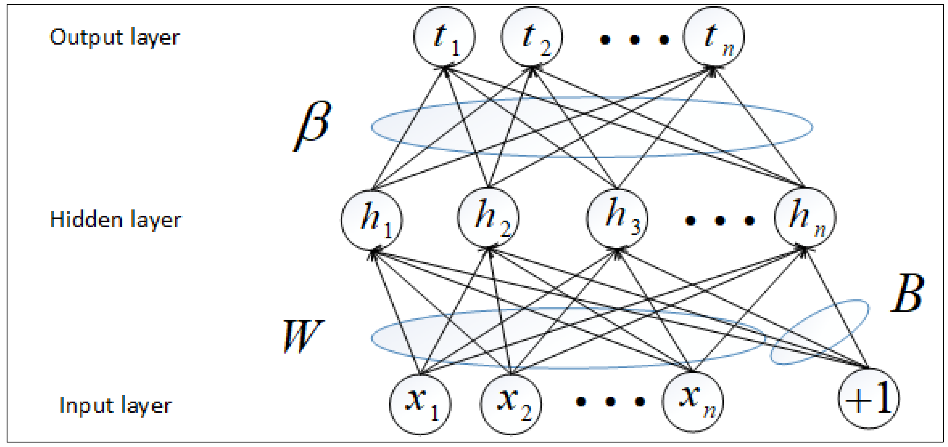
The ELM model was recently developed based on the single hidden layer with random weight configuration that was proposed by Prof. G. B. Huang et al. in 2006 and then extended to “generalized” single layer feed forward networks (SLFNs), where the hidden layer neurons need not be neuron alike [39,40]. The hidden neuron’s connection parameters are randomly generated without any iterative tuning and are independent of the data [41]. The network topology of ELM is shown in Figure 2.

Given a training set with N distinct samples $\Gamma =\left\{\left(x_j,t_j\right)|x_j\in {ℝ}^n,t_j\in {ℝ}^m,\mathrm{j}=1,\dots ,N\right\}$, where X is the predictive variable with dimension n and t is the objective variable with dimension m, the mathematical model of SLFNs with M hidden neurons and an activation function G(·) are described as:

$${\displaystyle \sum _{i=1}^n{\beta }_{i}G\left(w_i,b_i,x_j\right)},j=1,2,\dots ,N$$

(2)

where $b_i\in R$ is the randomly assigned bias of the ith hidden node and $w_i\in R$ is the randomly assigned input weight vector connecting the ith hidden node to the output node. $G\left(w_i,b_i,x_j\right)$ is the output of the ith hidden node with respect to the input sample $x_j$.

When the SLFN is completely approximating the data, that is, when the error between the output ${\widehat{t}}_o$ and the actual t_i is zero, the relationship is:

$${\displaystyle \sum _{i=1}^n{\beta }_{i}G\left(w_i,b_i,x_j\right)}={\mathrm{t}}_j,j=1,2,\dots ,N$$

(3)

The Equation (3) can be written as:

$$H\beta =T$$

(4)

where,

$$H=[{\mathrm{h}}_1^T{\mathrm{h}}_2^T\cdots {\mathrm{h}}_N^T]={\left[\begin{array}{ccc}G\left(w_1,b_1,x_1\right)& \cdots & G\left(w_n,b_n,x_1\right)\\ ⋮& \ddots & ⋮\\ G\left(w_1,b_1,x_N\right)& \cdots & G\left(w_n,b_n,x_N\right)\end{array}\right]}_{N\times n}$$

(5)

$$\beta ={\left[\begin{array}{c}{\beta }_1^T\\ {\beta }_2^T\\ ⋮\\ {\beta }_N^T\end{array}\right]}_{n\times m}T={\left[\begin{array}{c}{t}_1^T\\ t_2^T\\ ⋮\\ t_N^T\end{array}\right]}_{N\times m}$$

(6)

The output weights can be computed by finding the least-square solutions of the SLFNs in Equation (4), which is given as:

$$\beta =H^{†}T$$

(7)

where $H^{†}$ is the Moore–Penrose generalized inverse of the matrix $H$. If $H^{T}H$ is not singular matrix, then, Equation (7) can be written as:

$$\beta =H^{†}T={\left(H^{T}H\right)}^{-1}{H}^{T}T$$

(8)

In addition, we add an l − 2 regularization constraint to the loss function of ELM which can improve the generalization and robustness. equation (8) becomes the following formula:

$$\beta =\{\begin{array}{ll}{H}^T{\left(\frac{I}{C}+H^{T}H\right)}^{-1}T& ifN\le L\\ {\left(\frac{I}{C}+H^{T}H\right)}^{-1}{H}^{T}T& ifN>L\end{array}$$

(9)

where C assigns the regularization, I assigns the unit matrix, N assigns the number of samples and L assigns the number of hidden layer neurons.

Unfortunately, ELM is a batch learning algorithm. However, in practical applications such as solar radiation prediction, stock price prediction, and weather prediction, the time series data often arrives in the form of a data stream and may never end. The potential distribution and changing trend of the data continuously changes with time. When obtaining new data, traditional artificial intelligence algorithms such as artificial neural networks, support vector machines and extreme learning models, need to gather both old and new data to retrain [42]. Therefore, it is difficult to address “big data” and non-stationary and time-varying time series prediction problems.

To effectively solve the nonstationary time series problem of a data stream, the online sequential extreme learning machine (OS-ELM) was developed. The learning of OS-ELM includes a preliminary ELM batch learning process and a continuous one-by-one or block-by-block learning process.

Since OS-ELM involves the calculation of inversion during the update learning process, once the autocorrelation matrix of the hidden layer output matrix is singular or ill-conditioned, the generalization ability of OS-ELM will be severely degraded. Therefore, Huynh [16] combined Tikhonov regularization with OS-ELM and proposed a regularization of OS-ELM to improve the stability and generalization of the algorithm. To address the role of new samples in the process of online learning, the concept of the forgetting factor [43] was introduced to OS-ELM to strengthen the role of new samples by forgetting old samples, so that the updated predictive model is closer to the current state of the time-varying system.

Theoretically, the R-ELM-FF algorithm is equivalent to minimizing the following least squares loss function with FF and $l2$ regularization:

$$J_{FR}\left({\beta }_k\right)={\displaystyle \sum _{i=1}^k{\lambda }^{k-i}{\left|t_i-h_i{\beta }_k\right|}^2}+\delta {\lambda }^k{\Vert {\beta }_k\Vert }^2$$

(10)

where λ is the FF parameter with the weight of the old and new samples and δ is the regularization parameter, which can improve the stability and generalization ability of the algorithm.

Using the recursive least squares method to solve Equation (10), and the recursive calculation formula [18], ${\beta }_k$ can be deduced as:

$$\begin{array}{l}{P}_k=\frac{P_{k-1}}{\lambda }-\frac{P_{k-1}{h}_k^T{h}_k{P}_{k-1}}{\lambda \left(\lambda +h_k{P}_{k-1}{h}_k^T\right)}\\ {\beta }_k={\beta }_{k-1}+P_k{h}_k^T\left(t_k-h_k{\beta }_{k-1}\right)\end{array}$$

(11)

However, as time k increases, $\delta {\lambda }^k{\Vert {\beta }_k\Vert }^2$ decreases exponentially and trends toward zero, which will cause the regularization function to fade to failure. FOS-ELM introduces a new constant coefficient regularization term $\delta {\Vert {\beta }_k\Vert }^2$ in its cost function to replace the exponential regularization term $\delta {\lambda }^k{\Vert {\beta }_k\Vert }^2$. Its cost function is expressed as follows:

$$J_{FR}\left({\beta }_k\right)={\displaystyle \sum _{i=1}^k{\lambda }^{k-i}{\left|t_i-h_i{\beta }_k\right|}^2}+\delta {\Vert {\beta }_k\Vert }^2$$

(12)

The FOS-ELM works as follows:

Assume that the data sample arrives as a data stream; the activation function is $G\left(w,b,x\right)$, the number of hidden neurons is n, the regularization parameter is $\delta$, and the forgetting factor is $\lambda$.

Step 1: Initialization. Given the initial training subset ${\Omega }_{k-1}=\left\{\left(x_j,t_j\right)|x_j\in {ℝ}^n,t_j\in {ℝ}^m,\mathrm{j}=1,\dots ,k-1\right\}$, proceed as follows:

(1)

Generate the hidden layer neuron parameters randomly

$$\left(w_i,b_i\right),i=1,2,\cdots ,n$$

(2)

Compute the hidden layer output matrix by Equation (5)

$$H_{k-1}={[{\mathrm{h}}_1^T{\mathrm{h}}_2^T\cdots {\mathrm{h}}_{k-1}^T]}^T$$

(3)

Calculate the initial output weight matrix

$${\beta }_{k-1}=P_{k-1}{H}_{k-1}^T{T}_{k-1}$$

where

$$P_{k-1}={\left(H_{k-1}^T{H}_{k-1}+\lambda I\right)}^{-1},T_{k-1}={\left[t_1{t}_2\cdots t_{k-1}\right]}^T$$

Step 2: Online learning and prediction. Perform the following steps for the new sample $\left(x_k,t_k\right)$:

(1)

Compute the hidden layer output vector for the new sample input $x_k$: $h_k=\left[G\left(a_1,b_1,x_k\right)\cdots G\left(a_n,b_n,x_k\right)\right]$

(2)

Calculate the network output, that is, the predicted value of $t_k$: ${\widehat{t}}_k=h_k{\beta }_{k-1}$

(3)

Update the output weight by the actual label $t_k$

$$\begin{array}{l}{P}_k^{*}=\frac{1}{\lambda }{P}_{k-1}-\frac{\delta \left(1-\lambda \right)}{{\lambda }^2}{P}_{k-1}\left(I-\frac{\delta \left(1-\lambda \right)}{\lambda }{P}_{k-1}\right)P_{k-1}\\ P_k=P_k^{*}-\frac{P_k^{*}{h}_k^T{h}_k{P}_k^{*}}{1+h_k{P}_k^{*}{h}_k^T}\\ {\beta }_k={\beta }_{k-1}+P_k{h}_k^T\left(t_k-h_k{\beta }_{k-1}\right)-\delta \left(1-\lambda \right)P_k{\beta }_{k-1}\end{array}$$

(4)

Return to Step 2.

3.3. Procedures of the Methodology

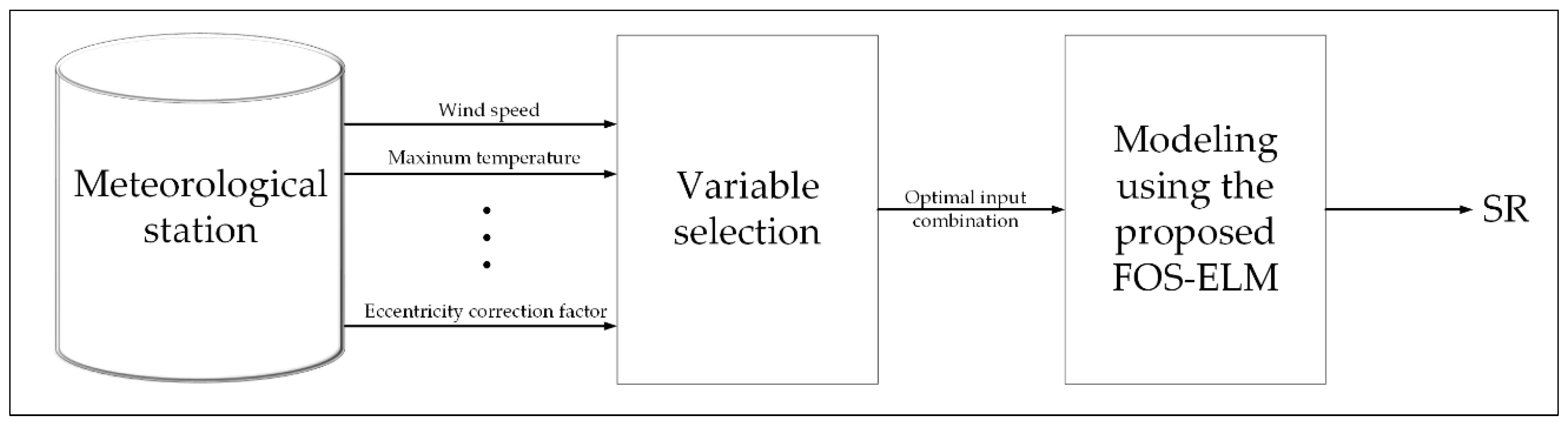
As illustrated in Figure 3, the structure of the applied methodology was reported starting with meteorological data collection, correlated input combination selection and the applied predictive model. The applied algorithm was conducted using Matlab software environment (R2017b, MathWorks, Natick, MA, USA).

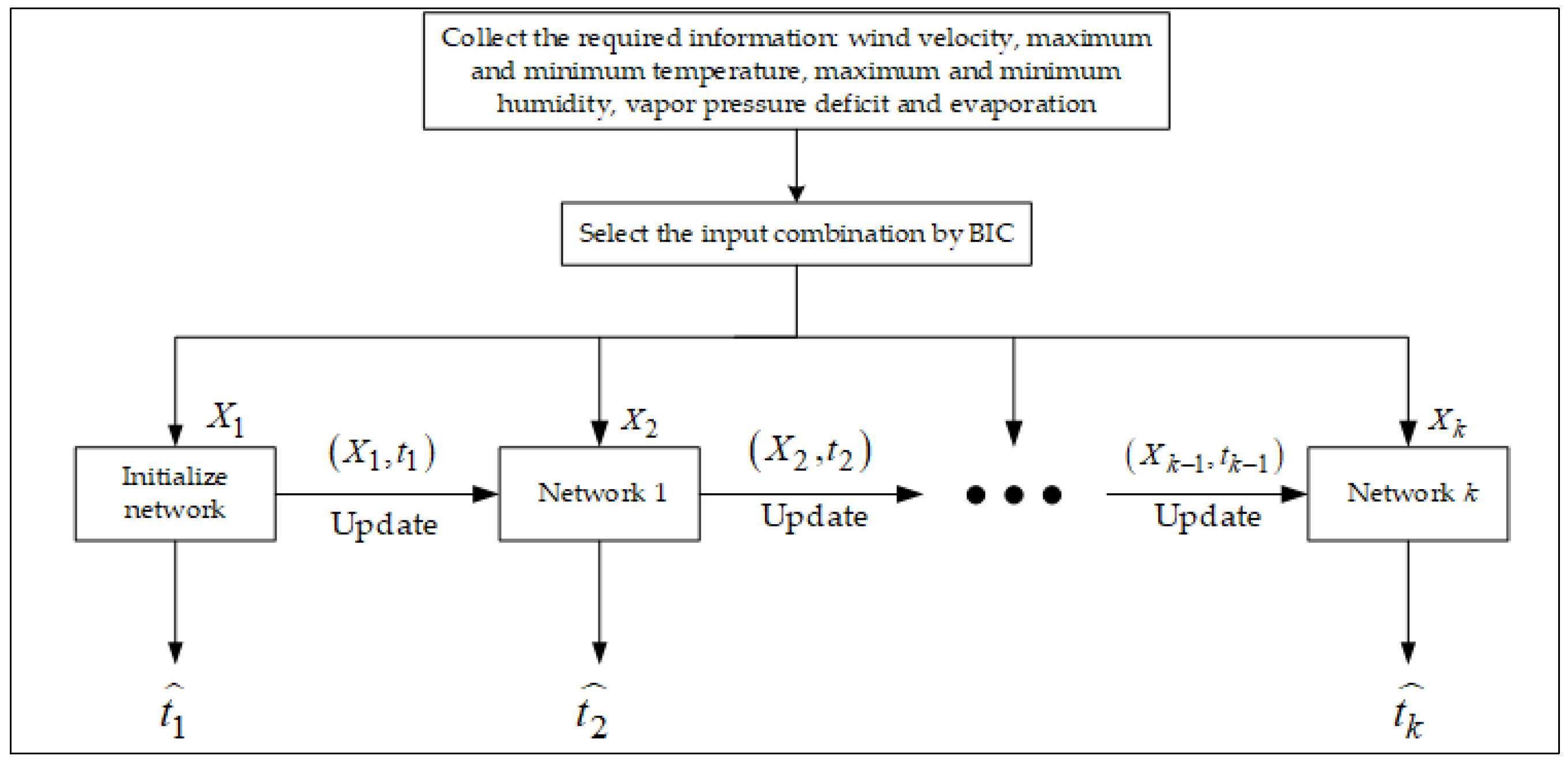
During the variable selection phase, the various input combinations were designed by calculating the BIC value. In the modeling stage, the proposed FOS-ELM algorithm was used to construct the solar radiation predictive model. Subsequently, these predictive models were trained through existing initial dataset. For each subsequent day, models predicted the solar radiation value for the next day and the model parameters were calibrated. This part of workflow and its flowchart can be seen in Figure 4.

3.4. Modeling Performance Indicators

To assess the developed FOS-ELM and the classical ELM models for the solar radiation prediction, multiple statistical indicators were examined. These performance indicators can be described mathematically as follows [44,45,46].

• The Correlation coefficient (r) is represented as:

  $$r=\left(\frac{{\displaystyle \sum _{k=1}^n\left(S{R}_{OBS,k}-{\stackrel{\_}{SR}}_{OBS,k}\right)\left(S{R}_{FOR,k}-{\stackrel{\_}{SR}}_{FOR,k}\right)}}{\sqrt{{\displaystyle \sum _{k=1}^n{\left(S{R}_{OBS,k}-{\stackrel{\_}{SR}}_{OBS,k}\right)}^2}}\sqrt{{\displaystyle \sum _{k=1}^N{\left(S{R}_{FOR,k}-{\stackrel{\_}{SR}}_{FOR,k}\right)}^2}}}\right)$$

  (13)
• The Willmott’s Index (WI) can be written as:

  $$WI=1-\left[\frac{{\displaystyle \sum _{k=1}^n{\left(S{R}_{FOR,k}-S{R}_{OBS,k}\right)}^2}}{{\displaystyle \sum _{k=1}^n{\left(\left|S{R}_{FOR,k}-{\stackrel{\_}{SR}}_{OBS,k}\right|+\left|S{R}_{OBS,k}-{\stackrel{\_}{SR}}_{OBS,k}\right|\right)}^2}}\right],0\le WI\le 1$$

  (14)
• The Nash–Sutcliffe efficiency (NS_E) is described as:

  $$N{S}_E=1-\left[\frac{{\displaystyle \sum _{k=1}^n{\left(S{R}_{OBS,k}-S{R}_{FOR,k}\right)}^2}}{{\displaystyle \sum _{k=1}^n{\left(S{R}_{OBS,k}-{\overline{SR}}_{FOR,k}\right)}^2}}\right],0\le N{S}_E\le 1$$

  (15)
• The root mean square error (RMSE) is given as:

  $$RMSE=\sqrt{\frac{1}{n}{\displaystyle \sum _{k=1}^n{\left(S{R}_{FOR,k}-S{R}_{OBS,k}\right)}^2}}$$

  (16)
• The mean absolute error (MAE) can be shown as:

  $$MAE=\frac{1}{n}{\displaystyle \sum _{k=1}^n\left|\left(S{R}_{FOR,k}-S{R}_{OBS,k}\right)\right|}$$

  (17)
• The Legates and McCabe’s (LM) agreement is stated as:

  $$LM=1-\left[\frac{{\displaystyle \sum _{k=1}^n\left|S{R}_{FOR,k}-S{R}_{OBS,k}\right|}}{{\displaystyle \sum _{k=1}^n\left|S{R}_{OBS,k}-{\stackrel{\_}{SR}}_{OBS,k}\right|}}\right],0\le LM\le 1$$

  (18)
• The relative root mean square error (RRMSE; %) is given as:

  $$RRMSE=\frac{\sqrt{\frac{1}{n}{\displaystyle \sum _{k=1}^n{\left(S{R}_{FOR,k}-S{R}_{OBS,k}\right)}^2}}}{\frac{1}{n}{\displaystyle \sum _{k=1}^n\left(S{R}_{OBS,k}\right)}}\times 100$$

  (19)
• The relative mean absolute percentage error (RMAE; %), is given as:

  $$RMAE=\frac{1}{n}{\displaystyle \sum _{k=1}^n\left|\frac{\left(S{R}_{FOR,k}-S{R}_{OBS,k}\right)}{S{R}_{OBS,k}}\right|}\times 100$$

  (20)

  where $S{R}_{OBS,k}$ and $S{R}_{FOR,k}$ are represented the observed and predicted kth data point of the solar radiation; whereas, ${\overline{SR}}_{OBS,k}$ and ${\overline{SR}}_{FOR,k}$ are the average values. n indicates the number of testing data.

4. Application, Results and Analysis

Results are presented for assessing the proposed FOS-ELM model for the solar radiation prediction. The proposed FOS-ELM model is appraised in comparison with the ELM model, using statistical metrics, diagnostic plots and error distributions between the observed and predicted solar radiation values over the testing phase.

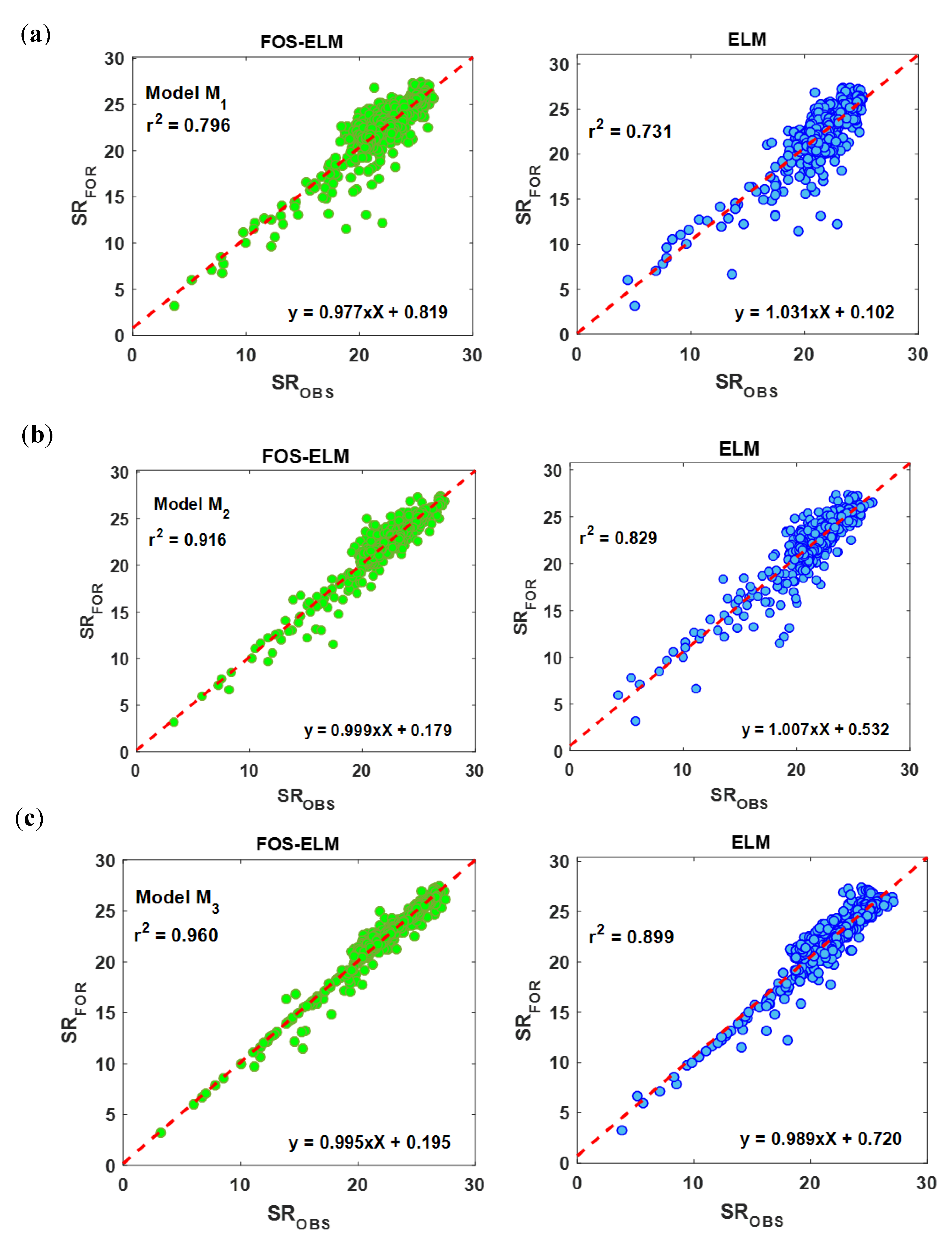
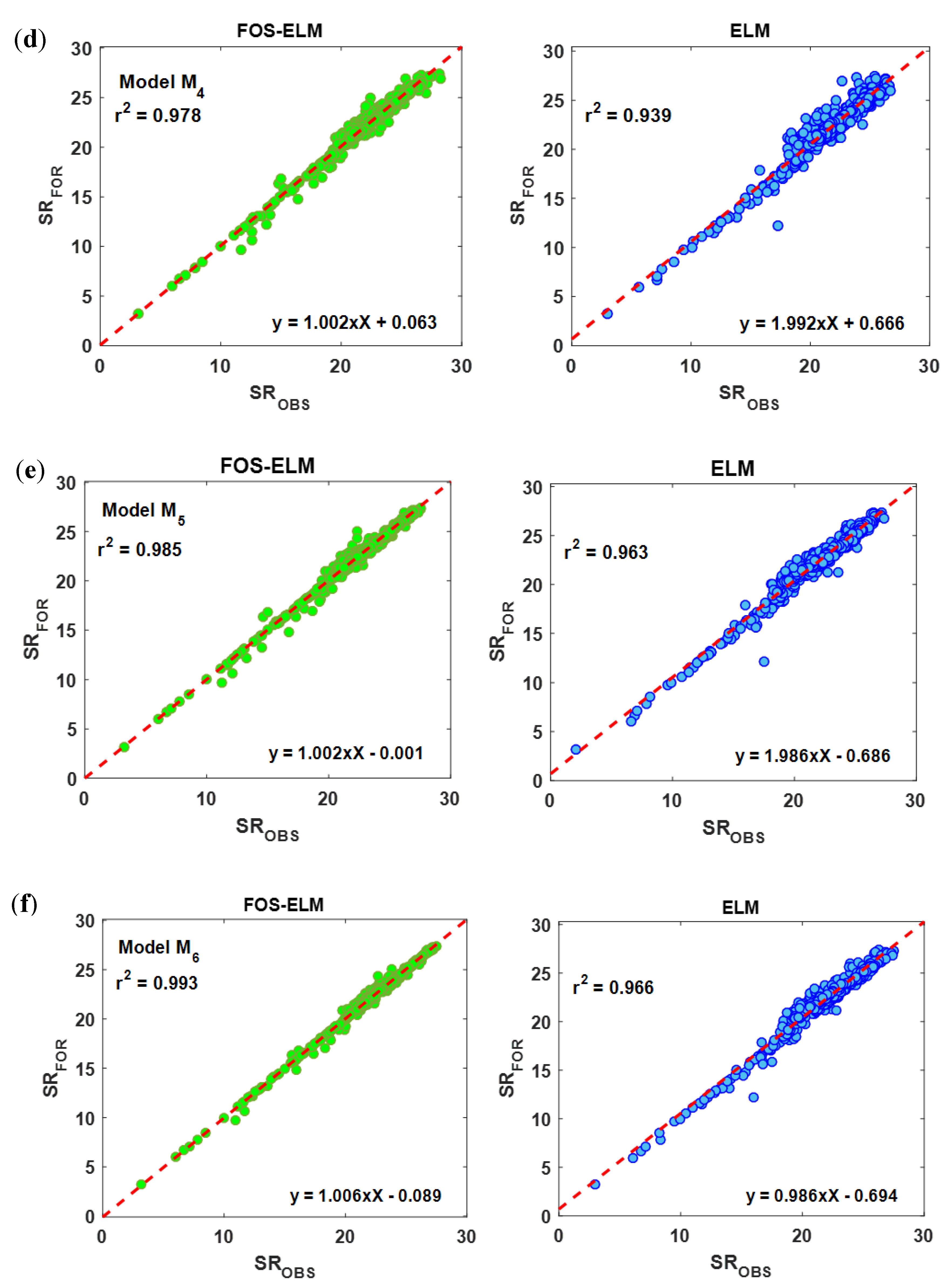
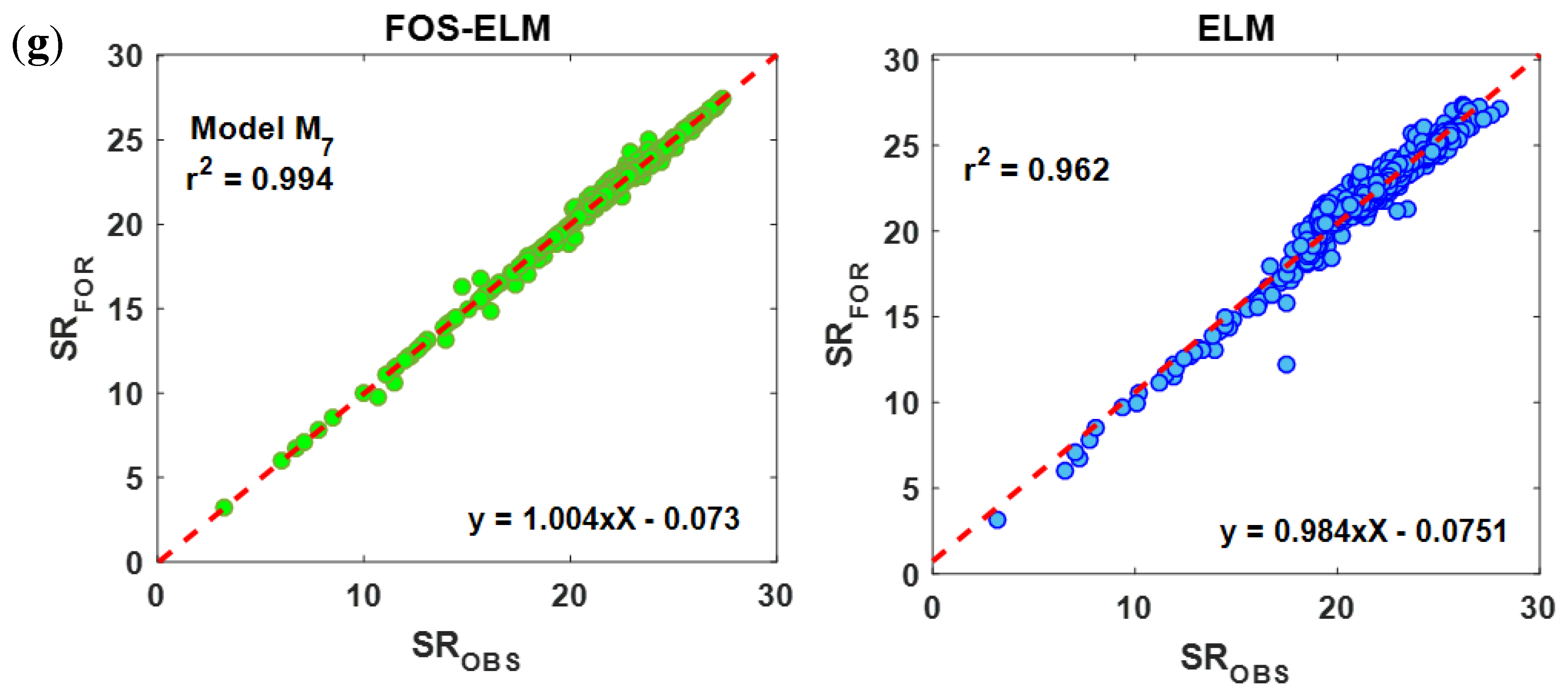
Figure 5 indicates the goodness-of-fit and correlation coefficient r² observed and predicted solar radiation through scatterplot. The proposed FOS-ELM method outperforms ELM in terms of r² (FOS-ELM ≈ 0.994, ELM ≈ 0.962) for model M₇ using all inputs. Again, the proposed FOS-ELM model is more accurate for M₆ model with input combination (W_speed, T_min, H_max, H_min, E_o, V_PD) attaining r² (FOS-ELM ≈ 0.993, ELM ≈ 0.966), followed by M₅, M₄, M₃, M₂ and M₁ models, respectively. On the basis of attaining the larger r²-value, the proposed FOS-ELM model shows better accuracy by incorporating all inputs (see; M₇) by generating the larger r²-value.

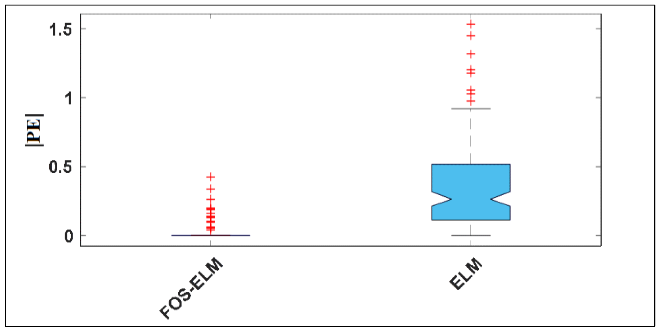
Figure 6 compares boxplots of the proposed FOS-ELM model with the ELM model for the most accurate M₇ model with all input combinations. The + denotes the outliers prediction error |PE| values together with their upper quartile, median, and lower quartile. The |PE|, confirmed with a much smaller quartile, was acquired by the FOS-ELM for M₇ model with all input utilization followed by the ELM model. By observing Figure 6, the accuracy of the proposed FOS-ELM is superior to the comparative model.

Calculating the model’s BIC value of all input variable combinations, the variable combination with the smallest BIC value is the optimal combination of variables. For different numbers of input variables, seven different models are constructed based on the optimal input combination, including the model with all input variables.

In

Table 1. The constructed seven input combination model based on the variability influential of each climate information (Several statistical metrics are computed as determination factors. Note, bold line is the best input combination.

Model	Input Combinations	Variable Forgetting Factor (FOS-ELM)			Extreme Learning Machine (ELM)
		Root Mean Square Error (RMSE)	Mean Absolute Error (MAE)	r	RMSE	MAE	r
M1	Eo	1.622	1.163	0.891	1.966	1.533	0.855
M2	Wsped + Eo	1.034	0.727	0.956	1.601	1.226	0.911
M3	Wspeed + VPD + Eo	0.707	0.449	0.979	1.227	0.875	0.947
M4	Wspeed + Tmin + Hmin + Eo	0.536	0.347	0.989	1.017	0.696	0.968
M5	Wspeed + Tmin + Hmin + VPD + Eo	0.429	0.245	0.993	0.791	0.570	0.981
M6	Wspeed + Tmin + Hmax + Hmin + VPD + Eo	0.287	0.143	0.997	0.788	0.565	0.981
M7	ALL	0.259	0.118	0.997	0.831	0.586	0.979

, the preciseness of FOS-ELM is evaluated in comparison to the ELM method for each input combination on the basis of r, RMSE and MAE. The proposed FOS-ELM model applied with all input utilization (model M₇) attained the highest correlation coefficient and smallest RMSE and MAE (r ≈ 0.997, RMSE ≈ 0.259, MAE ≈ 0.118) compared to the ELM (r ≈ 0.979, RMSE ≈ 0.831, MAE ≈ 0.586) model. Moreover, for M₆, these metrics were FOS-ELM (r ≈ 0.997, RMSE ≈ 0.287, MAE ≈ 0.143), followed ELM (r ≈ 0.981, RMSE ≈ 0.788, MAE ≈ 0.565). Similarly, the FOS-ELM model is better for (M₁, …, M₅) in terms of achieving largest magnitudes of r and smallest magnitudes of RMSE and MAE. This is a clear indication that the proposed FOS-ELM model can be considered to be a better data-intelligent tool for solar radiation prediction than the ELM model.

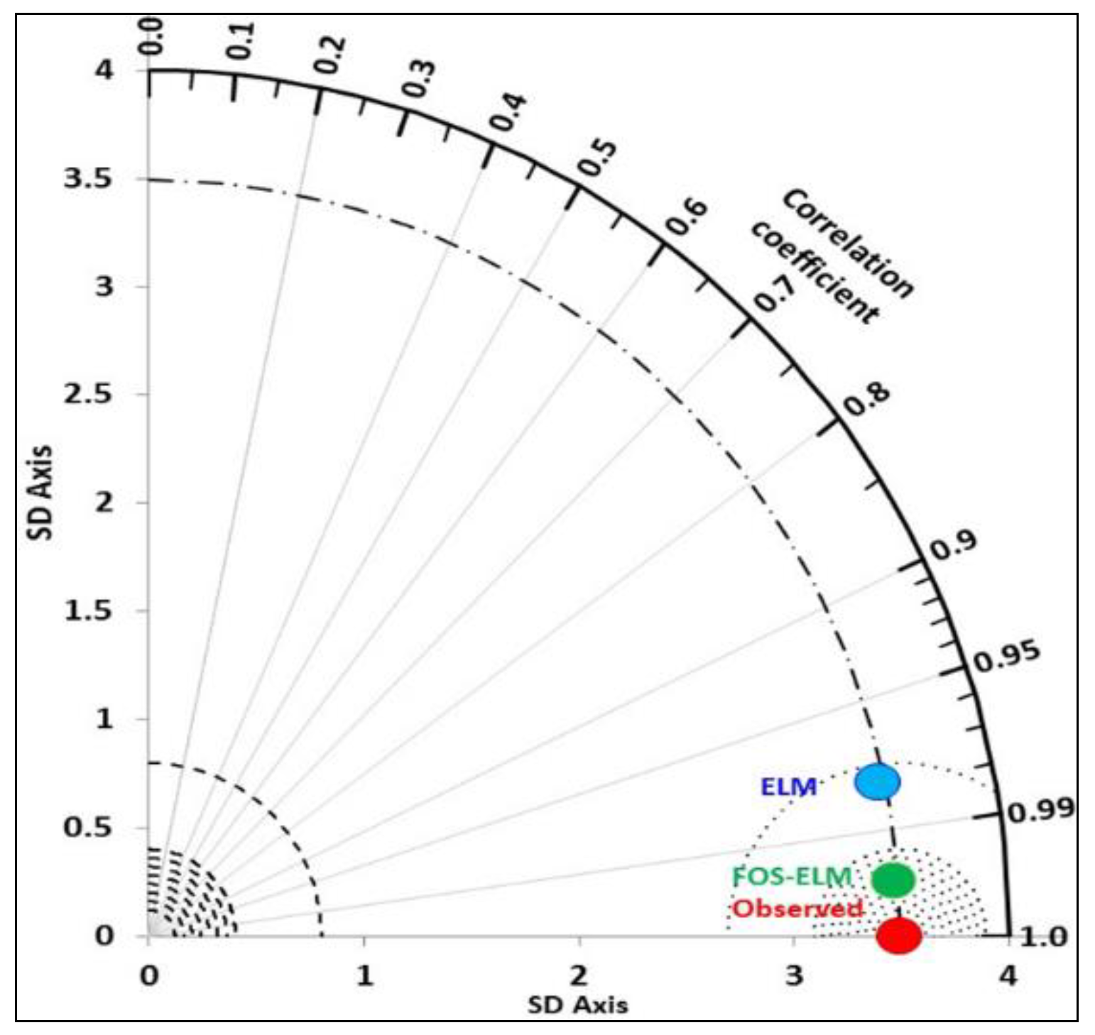
In Figure 7, the Taylor diagram presents the statistical summary of the observed and predicted solar radiation on the basis of their correlation coefficient (r). For all input combination M₇, the magnitude of r for FOS-ELM was approximately 0.997, compared to ELM ≈ 0.98. The FOS-ELM was seen closer to the observed SR, compared to ELM. Overall, the r of the proposed FOS-ELM exhibits more accuracy to the observed SR.

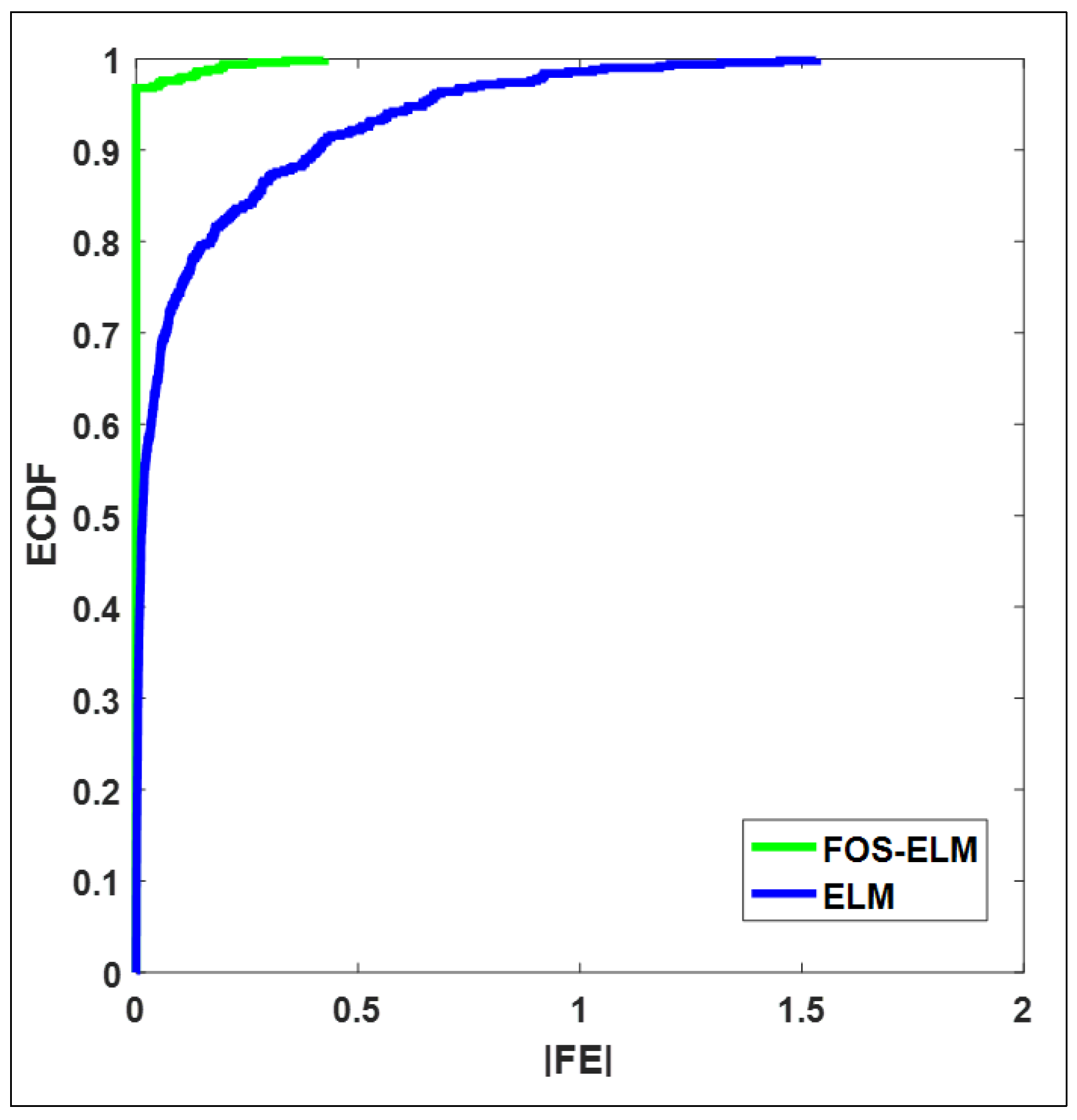
The preciseness of the FOS-ELM and ELM models is evaluated for different input combinations in terms of WI, NS_E and LM, shown in

Table 2. Test modeling phase performance of FOS-ELM and ELM models using all the reported metrics. Note, the best model is boldfaced.

Model	Input Combinations	Variable Forgetting Factor (FOS-ELM)			Extreme Learning Machine (ELM)
		NSE	WI	LM	NSE	WI	LM
M1	Eo	0.784	0.919	0.507	0.682	0.883	0.351
M2	Wsped + Eo	0.912	0.968	0.692	0.790	0.926	0.481
M3	Wspeed + VPD + Eo	0.959	0.985	0.810	0.876	0.957	0.629
M4	Wspeed + Tmin + Hmin + Eo	0.976	0.992	0.853	0.915	0.971	0.705
M5	Wspeed + Tmin + Hmin + VPD + Eo	0.985	0.995	0.896	0.949	0.982	0.759
M6	Wspeed + Tmin + Hmax + Hmin + VPD + Eo	0.993	0.998	0.939	0.949	0.982	0.761
M7	ALL	0.994	0.998	0.950	0.943	0.981	0.752

. The proposed FOS-ELM model with input combination M₇ attained the highest values of NS_E ≈ 0.994, WI ≈ 0.998, and LM ≈ 0.950, followed by ELM (NS_E ≈ 0.943, WI ≈ 0.981, and LM ≈ 0.752). For other input combinations, again the FOS-ELM model exhibited high accuracy. The proposed FOS-ELM model outperformed the ELM model. In Figure 8, the empirical cumulative distribution function (ECDF) for the best input combination M₅ depicts the different prediction skills. The proposed FOS-ELM method was reasonably superior to the ELM model. Based on the error bracket (0 to ± 2) for M₅, Figure 8 clearly proves that the FOS-ELM was the extreme accurate model.

Geographically, the FOS-ELM vs. ELM model demonstrate the magnitudes of RRMSE and RMAE metrics for all investigated input combinations (See

Table 3. Numerical comparison between FOS-ELM and ELM models based (RRMSE, %) and the (RMAE, %) computed within the test sites. Note that the best model is boldfaced.

Model	Testing Period	Variable Forgetting Factor (FOS-ELM)		Extreme Learning Machine (ELM)
	Input Combination	Relative Root Mean Square Error (RRMSE) (%)	Relative Mean Absolute Percentage Error (RMAE) (%)	RRMSE (%)	RMAE (%)
M1	Eo	7.381	5.650	8.947	7.497
M2	Wsped + Eo	4.704	3.528	7.283	6.108
M3	Wspeed + VPD + Eo	3.218	2.157	5.581	4.127
M4	Wspeed + Tmin + Hmin + Eo	2.440	1.639	4.629	3.198
M5	Wspeed + Tmin + Hmin + VPD + Eo	1.952	1.176	3.597	2.734
M6	Wspeed + Tmin + Hmax + Hmin + VPD + Eo	1.305	0.686	3.584	2.646
M7	ALL	1.179	0.574	3.780	2.748

). M₇ reported the best prediction results for the solar radiation prediction using the proposed predictive model. Quantitatively, (RRMSE ≈ 1.179%) and (RMAE ≈ 0.574%) on the basis of RRMSE and RMAE. The FOS-ELM model was seen to generate minimal values of the examined absolute error indicators. Overall, the prediction errors generated by the proposed FOS-ELM model were low in terms of their relative error values, but more importantly, they were within the recommended range of a 10% threshold for an excellent model classification [47].

5. Discussion: Limitations and Further Remarks

In this paper, the suitability of the FOS-ELM benchmarked with the ELM for daily solar radiation prediction was investigated. The FOS-ELM outperformed the ELM model for the selected region, revealing that the FOS-ELM model was efficient in utilizing the meteorological data as inputs to predict solar radiation. The FOS-ELM model, being a robust hybrid AI algorithm, is able to extract vital information from the meteorological variables, and subsequently simulates the stochastic and complex behavior of solar radiation. The FOS-ELM model has been proven to yield good performance with high prediction accuracy. The benefit of the FOS-ELM model is that it efficiently approximates numerous linear or nonlinear systems without predefining the constraints of climate input data or target solar radiation.

Coal and oil are normally considered for non-renewable energy sources of electricity generation to meet the marked demands. The intermittent availability is a challenging problem to all renewable energy sources. Solar energy in the form of solar radiation is a naturally available renewable energy resource which has the lowest environmental impact [3]. However, the solar energy is only available during daylight hours, which is aggravated by the highly variable availability owing to environmental and meteorological factors that have obvious correlations [29]. The FOS-ELM can successfully adapt to design the new smart grids to predict the demand and supply needs which can reduce the downtimes and enhance efficiency.

Moreover, the Paris climate agreement has recently urged the use of cleaner renewable energy to reduce carbon emissions. Hence, a more reliable production of electricity from these renewable energies is predetermined. Consequently, the smart grids incorporating the FOS-ELM model could handle this challenge to predict accurately in order to generate electricity from renewable energy.

6. Conclusions

In this work, a novel ELM-based model, a regularized online sequential extreme learning machine with variable forgetting factor, was proposed and first applied to daily global solar radiation prediction. Using wind speed, maximum and minimum temperature, maximum and minimum humidity vapor pressure, and the eccentricity correction factor as seven different input variables of this study, we investigated the correlation between different variables and solar radiation and the influence of different input combinations on the prediction accuracy of the model, and selected the optimal model input combination with a different number of input variables by BIC. The statistical performance evaluation indicates that global solar radiation prediction accuracy can achieve excellent prediction accuracy with wind speed, minimum temperature, maximum and minimum humidity vapor pressure and the eccentricity correction factor as input variables (RRMSE ≈ 1.305%, RMAE ≈ 0.686%, RRMSE ≈ 3.584%, RMAE ≈ 2.646%, R ≈ 0.997). Compared with ELM, the results clearly demonstrate the effectiveness and outstanding performance of the proposed FOS-ELM model. Compared with the papers mentioned in the literature, the proposed model develops a new way to deal with complex non-stationary time series. The proposed model tries to update the output weight of the network and “fix” the network model every day to achieve higher prediction accuracy. However, References [22,32] reported in the literature optimized the network structure and initialization weights through different methods, such as a genetic algorithm, etc. Therefore, for future work, we will try to develop models based on an optimal network structure of online learning, including but not limited to optimizing the number of hidden layer neurons and multiple hidden layer neural networks. We will also introduce more meteorological factors in order to improve prediction accuracy.

References

- Arto, I.; Capellán-Pérez, I.; Lago, R.; Bueno, G.; Bermejo, R. The energy requirements of a developed world. Energy Sustain. Dev. 2016, 33, 1–13. [Google Scholar] [CrossRef]
- OECD. International Energy Agency Energy Policies of IEA Countries: Sweden 2013 Review; OECD Publishing: Paris, France, 2013. [Google Scholar] [CrossRef]
- Bailis, R.; Drigo, R.; Ghilardi, A.; Masera, O. The carbon footprint of traditional woodfuels. Nat. Clim. Chang. 2015, 5, 266–272. [Google Scholar] [CrossRef]
- Brinkworth, B.J. Solar energy. Nature 1974, 249, 726–729. [Google Scholar] [CrossRef]
- Stone, K.D.; Flynn, R.W.; Cook, J.A. Post-glacial colonization of northwestern North America by the forest-associated American marten (Martes americana, Mammalia: Carnivora: Mustelidae). Mol. Ecol. 2002, 11, 2049–2063. [Google Scholar] [CrossRef] [PubMed]
- Acar, C.; Dincer, I. Comparative assessment of hydrogen production methods from renewable and non-renewable sources. Int. J. Hydrogen Energy 2014, 39, 1–12. [Google Scholar] [CrossRef]
- Samuel Chukwujindu, N. A comprehensive review of empirical models for estimating global solar radiation in Africa. Renew. Sustain. Energy Rev. 2017, 78, 955–995. [Google Scholar] [CrossRef]
- Szabó, S.; Bódis, K.; Huld, T.; Moner-Girona, M. Energy solutions in rural Africa: Mapping electrification costs of distributed solar and diesel generation versus grid extension. Environ. Res. Lett. 2011, 6. [Google Scholar] [CrossRef]
- World Energy Council World Energy Resources: 2013 Survey. World Energy Counc. 2013, 11. Available online: http://www.worldenergy.org/wp-content/uploads/2013/09/Complete_WER_2013_Survey.pdf (accessed on 15 October 2018).
- Deo, R.C.; Wen, X.; Qi, F. A wavelet-coupled support vector machine model for forecasting global incident solar radiation using limited meteorological dataset. Appl. Energy 2016, 168, 568–593. [Google Scholar] [CrossRef]
- Salcedo-Sanz, S.; Deo, R.C.; Cornejo-Bueno, L.; Camacho-Gómez, C.; Ghimire, S. An efficient neuro-evolutionary hybrid modelling mechanism for the estimation of daily global solar radiation in the Sunshine State of Australia. Appl. Energy 2018, 209, 79–94. [Google Scholar] [CrossRef]
- Al-Shamisi, M.H.; Assi, A.H.; Hejase, H.A.N. Artificial neural networks for predicting global solar radiation in Al Ain City—UAE. Int. J. Green Energy 2013, 10, 443–456. [Google Scholar] [CrossRef]
- Zhang, J.; Zhao, L.; Deng, S.; Xu, W.; Zhang, Y. A critical review of the models used to estimate solar radiation. Renew. Sustain. Energy Rev. 2017, 70, 314–329. [Google Scholar] [CrossRef]
- Mihalakakou, G.; Santamouris, M.; Asimakopoulos, D.N. The total solar radiation time series simulation in Athens, using neural networks. Architecture 2000, 197, 185–197. [Google Scholar] [CrossRef]
- Rahimikhoob, A. Estimating global solar radiation using artificial neural network and air temperature data in a semi-arid environment. Renew. Energy 2010, 35, 2131–2135. [Google Scholar] [CrossRef]
- Bou-Rabee, M.; Sulaiman, S.A.; Saleh, M.S.; Marafi, S. Using artificial neural networks to estimate solar radiation in Kuwait. Renew. Sustain. Energy Rev. 2017, 72, 434–438. [Google Scholar] [CrossRef]
- Xue, X. Prediction of daily diffuse solar radiation using artificial neural networks. Int. J. Hydrogen Energy 2017, 42, 28214–28221. [Google Scholar] [CrossRef]
- Kumar, M.; Raghuwanshi, N.; Singh, R.; Wallender, W.; Pruitt, W. Estimating Evapotranspiration using Artificial Neural Network. J. Irrig. Drain. Eng. 2002, 128, 224–233. [Google Scholar] [CrossRef]
- Citakoglu, H. Comparison of artificial intelligence techniques via empirical equations for prediction of solar radiation. Comput. Electron. Agric. 2015, 118, 28–37. [Google Scholar] [CrossRef]
- Olatomiwa, L.; Mekhilef, S.; Shamshirband, S.; Petković, D. Adaptive neuro-fuzzy approach for solar radiation prediction in Nigeria. Renew. Sustain. Energy Rev. 2015, 51, 1784–1791. [Google Scholar] [CrossRef]
- Sumithira, T.R.; Nirmal Kumar, A. Prediction of monthly global solar radiation using adaptive neuro fuzzy inference system (ANFIS) technique over the State of Tamilnadu (India): A comparative study. Appl. Sol. Energy 2012, 48, 140–145. [Google Scholar] [CrossRef]
- Aybar-Ruiz, A.; Jiménez-Fernández, S.; Cornejo-Bueno, L.; Casanova-Mateo, C.; Sanz-Justo, J.; Salvador-González, P.; Salcedo-Sanz, S. A novel Grouping Genetic Algorithm-Extreme Learning Machine approach for global solar radiation prediction from numerical weather models inputs. Sol. Energy 2016, 132, 129–142. [Google Scholar] [CrossRef]
- Jagielski, R. Genetic Programming Prediction of Solar Activity. In Proceedings of the International Conference on Intelligent Data Engineering and Automated Learning, Hong Kong, China, 13–15 December 2000. [Google Scholar]
- Shavandi, H.; Saeedi Ramyani, S. A linear genetic programming approach for the prediction of solar global radiation. Neural Comput. Appl. 2013. [Google Scholar] [CrossRef]
- Wu, J.; Chan, C.K.; Zhang, Y.; Xiong, B.Y.; Zhang, Q.H. Prediction of solar radiation with genetic approach combing multi-model framework. Renew. Energy 2014. [Google Scholar] [CrossRef]
- Mohammadi, K.; Shamshirband, S.; Tong, C.W.; Arif, M.; Petković, D.; Sudheer, C. A new hybrid support vector machine-wavelet transform approach for estimation of horizontal global solar radiation. Energy Convers. Manag. 2015, 92, 162–171. [Google Scholar] [CrossRef]
- Deo, R.C.; Şahin, M. Forecasting long-term global solar radiation with an ANN algorithm coupled with satellite-derived (MODIS) land surface temperature (LST) for regional locations in Queensland. Renew. Sustain. Energy Rev. 2017, 72, 828–848. [Google Scholar] [CrossRef]
- Wang, J.; Xie, Y.; Zhu, C.; Xu, X. Solar radiation prediction based on phase space reconstruction of wavelet neural network. Procedia Eng. 2011, 15, 4603–4607. [Google Scholar] [CrossRef]
- Zhang, P.; Takano, H.; Murata, J. Daily solar radiation prediction based on wavelet analysis. In Proceedings of the SICE Annual Conference 2011, Tokyo, Japan, 13–18 September 2011. [Google Scholar]
- Mellit, A.; Benghanem, M.; Kalogirou, S.A. An adaptive wavelet-network model for forecasting daily total solar-radiation. Appl. Energy 2006. [Google Scholar] [CrossRef]
- Olatomiwa, L.; Mekhilef, S.; Shamshirband, S.; Mohammadi, K.; Petković, D.; Sudheer, C. A support vector machine-firefly algorithm-based model for global solar radiation prediction. Sol. Energy 2015, 115, 632–644. [Google Scholar] [CrossRef]
- Salcedo-Sanz, S.; Casanova-Mateo, C.; Pastor-Sánchez, A.; Sánchez-Girón, M. Daily global solar radiation prediction based on a hybrid Coral Reefs Optimization—Extreme Learning Machine approach. Sol. Energy 2014, 105, 91–98. [Google Scholar] [CrossRef]
- Wang, R.; Li, J.; Wang, J.; Gao, C. Research and application of a hybridwind energy forecasting system based on data processing and an optimized extreme learning machine. Energies 2018, 11. [Google Scholar] [CrossRef]
- Al-Dahidi, S.; Ayadi, O.; Adeeb, J.; Alrbai, M.; Qawasmeh, R.B. Extreme Learning Machines for Solar Photovoltaic Power Predictions. Energies 2018, 11. [Google Scholar] [CrossRef]
- REN21. Renewables 2015-Global Status Report; REN21: Pairs, France, 2015; Volume 4, ISBN 978-92-4-150061-6. [Google Scholar]
- REN21. Renewables 2017: Global Status Report; REN21: Pairs, France, 2017; Volume 72, ISBN 978-3-9818107-0-7. [Google Scholar]
- Saadi, N.; Miketa, A.; Howells, M. African Clean Energy Corridor: Regional integration to promote renewable energy fueled growth. Energy Res. Soc. Sci. 2015, 5, 130–132. [Google Scholar] [CrossRef]
- Schwarz, G. Estimating the Dimension of a Model. Ann. Stat. 1978. [Google Scholar] [CrossRef]
- Huang, G.-B.; Zhu, Q.-Y.; Siew, C.-K. Extreme learning machine: Theory and applications. Neurocomputing 2006, 70, 489–501. [Google Scholar] [CrossRef] [Green Version]
- Huang, G.B.; Chen, L. Convex incremental extreme learning machine. Neurocomputing 2007, 70, 3056–3062. [Google Scholar] [CrossRef]
- Sanikhani, H.; Deo, R.C.; Yaseen, Z.M.; Eray, O.; Kisi, O. Non-tuned data intelligent model for soil temperature estimation: A new approach. Geoderma 2018, 330, 52–64. [Google Scholar] [CrossRef]
- Crisosto, C.; Hofmann, M.; Mubarak, R.; Seckmeyer, G. One-Hour Prediction of the Global Solar Irradiance from All-Sky Images Using Artificial Neural Networks. Energies 2018, 11, 2906. [Google Scholar] [CrossRef]
- Paleologu, C.; Benesty, J.; Ciochiňa, S. A robust variable forgetting factor recursive least-squares algorithm for system identification. IEEE Signal Process. Lett. 2008. [Google Scholar] [CrossRef]
- Legates, D.R.; Mccabe, G.J. Evaluating the use of “goodness-of-fit” measures in hydrologic and hydroclimatic model validation. Water Resour. Res. 1999, 35, 233–241. [Google Scholar] [CrossRef]
- Willmott, C.J.; Matsuura, K. Advantages of the mean absolute error (MAE) over the root mean square error (RMSE) in assessing average model performance. Clim. Res. 2005, 30, 79–82. [Google Scholar] [CrossRef] [Green Version]
- Chai, T.; Draxler, R.R. Root mean square error (RMSE) or mean absolute error (MAE)?—Arguments against avoiding RMSE in the literature. Geosci. Model Dev. 2014, 7, 1247–1250. [Google Scholar] [CrossRef]
- Dan Foresee, F.; Hagan, M.T. Gauss-Newton approximation to bayesian learning. In Proceedings of the 1997 International Joint Conference on Neural Networks, Houston, TX, USA, 12 June 1997. [Google Scholar]
Figure 1.
The location of the studied meteorological station Bur Dedougou in Burkina Faso, West Africa.
Figure 2.
The network topology of classical extreme learning machine (ELM).
Figure 3.
Main frame of the proposed variable forgetting factor (FOS-ELM) for solar radiation prediction.
Figure 4.
Flowchart of the proposed methodology.
Figure 5.
Scatterplots variance between the observed and predicted solar radiation over the test modeling phase, variable forgetting factor (FOS-ELM) vs. extreme learning machine (ELM) models and for all the investigated input combination panels (a) M1, (b) M2, (c) M3, (d) M4, (e) M5, (f) M6 and (g) M7.
Figure 6.
Box-plots of the prediction error |PE| of the variable forgetting factor (FOS-ELM) vs. the extreme learning machine (ELM) model between the observed and predicted solar radiation for all input combination M7. PE.
Figure 7.
Two dimensions Taylor diagram illustration for the best input combination: xvariable forgetting factor (FOS-ELM) vs. extreme learning machine (ELM).
Figure 8.
Empirical cumulative distribution function (ECDF) of the prediction error, |PE| for all input combination M7 using the variable forgetting factor (FOS-ELM) vs. the extreme learning machine (ELM) model.