Scheduling Distributed Energy Resource Operation and Daily Power Consumption for a Smart Building to Optimize Economic and Environmental Parameters


Abstract
:1. Introduction
- We present a solution to the daily power consumption scheduling problem for household tasks over a finite time horizon and DER operation scheduling in a smart building composed of multiple smart homes.
- A mathematical formulation of the scheduling problem, based on a combination of several single-objective MILP techniques, with the aim of minimizing the conflicting goals of reducing CO2 emissions and total electricity costs is presented.
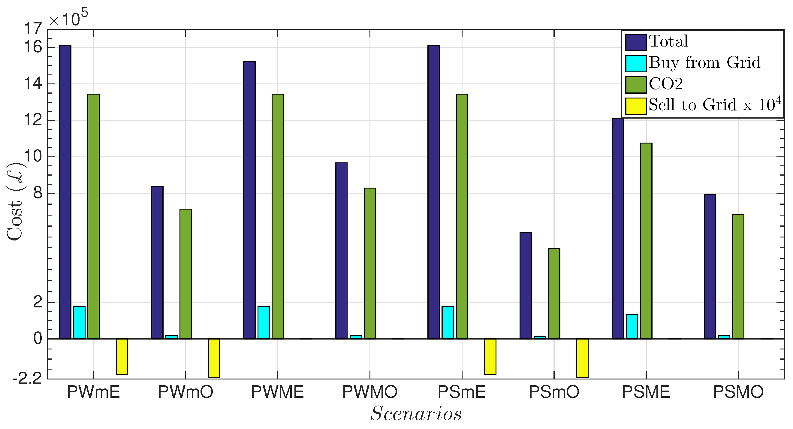
- We show that adding a DER system in a smart home environment leads to a significant reduction in electricity consumption and CO2 emissions.
- Extensive experiments to validate the efficacy of the proposed approach are presented.
2. Related Work
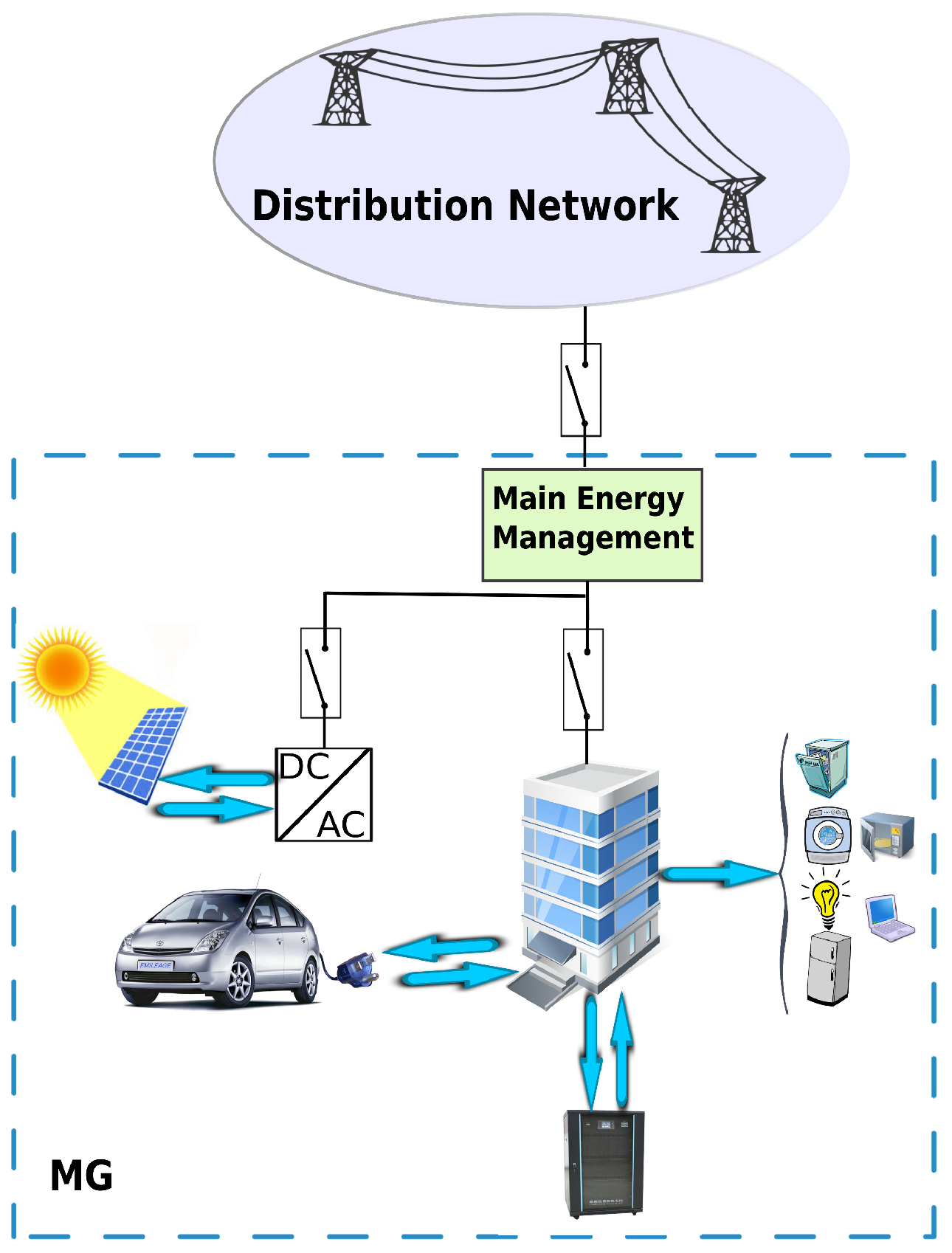
3. System Model
4. Appliance Scheduling Optimization Problem Formulation
4.1. Optimization Constraints
4.1.1. Execution Time Window for Each Appliance
4.1.2. Solar Panel
4.1.3. Energy Storage System
4.1.4. Energy Balances
4.1.5. Peak Demand Charge
4.1.6. User Time Preferences
4.2. Objective Functions
5. Performance Evaluation
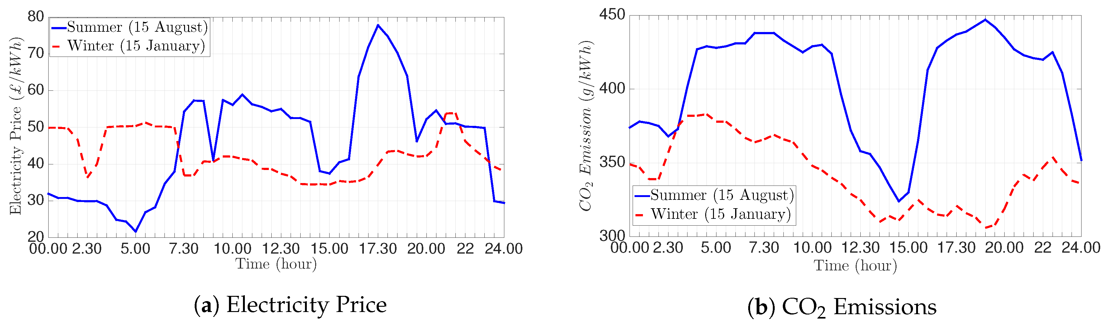
5.1. Experimental Setup
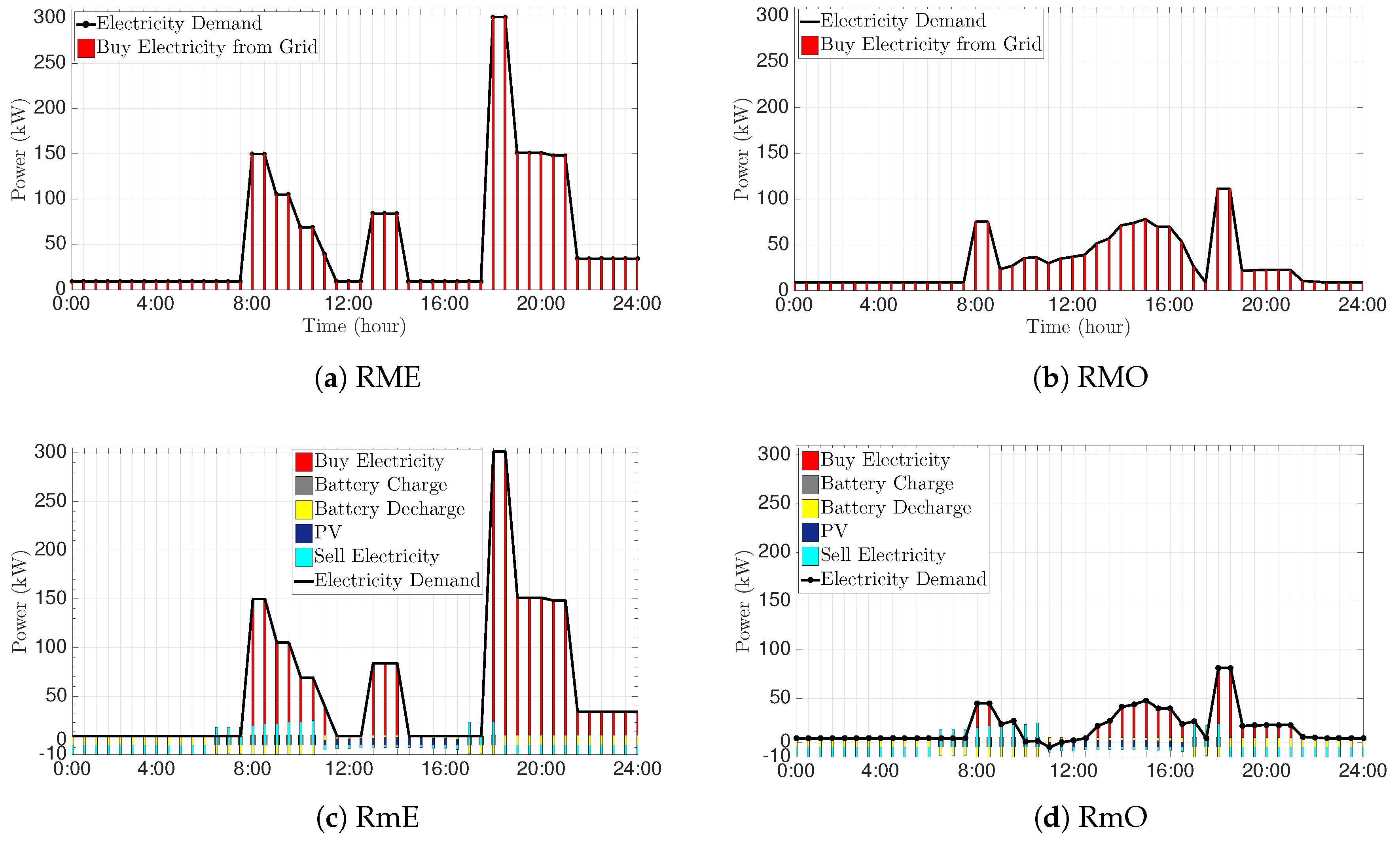
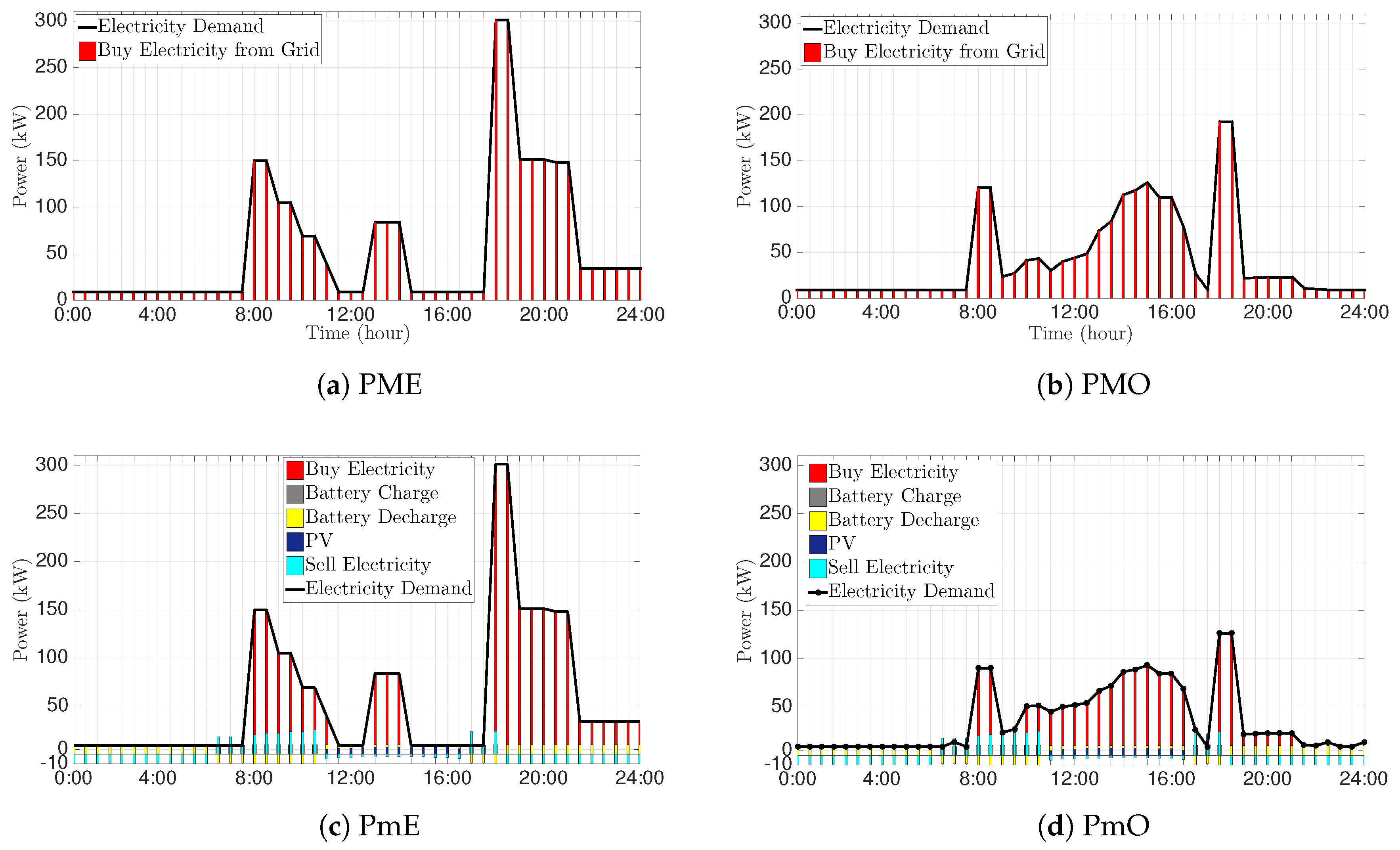
5.2. Performance Results
6. Conclusions and Future Directions
Supplementary Materials
Author Contributions
Acknowledgments
Conflicts of Interest
Nomenclature
| Binary Variables | |
| task i status of home j at time t | |
| Indices | |
| i | ask number |
| j | home number in the smart building |
| t | time interval |
| Parameters | |
| weighting factor of the multi-objective function | |
| weighting factor of the multi-objective function | |
| time interval duration h | |
| charge/discharge efficiency of the energy storage system | |
| intensity of the grid electricity at time t (kg CO/kWh) | |
| real-time price for buying electricity from the grid at time t (£/kWh) | |
| the difference between peak and base electricity demand price from the grid (£/kWh) | |
| C | operation and maintenance cost of the energy storage system (£/kWh) |
| operation and maintenance cost of photovoltaic panels (£/kWh) | |
| real-time price for selling electricity to the grid at time t (£/kWh) | |
| latest finishing time of task i in home j | |
| energy storage system capacity (kWh) | |
| energy storage system discharge limit (kW) | |
| processing time of task i in home j | |
| agreed electricity peak demand threshold from the grid (kW) | |
| earliest starting time of task i in home j | |
| Variables | |
| length of the load profile of an appliance | |
| daily electricity cost of a home (£) | |
| daily emissions (kg CO) | |
| energy storage system charge rate at time t (kW) | |
| energy storage system discharge rate at time t (kWh) | |
| electrical power bought from the grid at time t (kW) | |
| extra electrical load from the grid over the agreed threshold value (kW) | |
| initial state of the energy storage system (kW) | |
| electricity in the energy storage system at time t (kW) | |
| generated power by PV with solar irradiance R (kW) | |
| rated power of PV (kW) | |
| R | solar irradiance (W/m) |
| certain radiation point, usually set to 150 W/m | |
| solar radiation in the standard conditions, usually set to 1000 W/m |
References
- Rahimi, F.; Ipakchi, A. Demand response as a market resource under the smart grid paradigm. IEEE Trans. Smart Grid 2010, 1, 82–88. [Google Scholar] [CrossRef]
- Hajeforosh, S.F.; Pooranian, Z.; Shabani, A.; Conti, M. Evaluating the High Frequency Behavior of the Modified Grounding Scheme in Wind Farms. Appl. Sci. 2017, 7, 1323. [Google Scholar] [CrossRef]
- Katiraei, F.; Iravani, R.; Hatziargyriou, N.; Dimeas, A. Microgrids management. IEEE Power Energy Mag. 2008, 6, 54–65. [Google Scholar] [CrossRef]
- Fallah, S.N.; Deo, R.C.; Shojafar, M.; Conti, M.; Shamshirband, S. Computational Intelligence Approaches for Energy Load Forecasting in Smart Energy Management Grids: State of the Art, Future Challenges, and Research Directions. Energies 2018, 11, 596. [Google Scholar] [CrossRef]
- Moghaddam, A.A.; Rahimi-Kian, H.M. Optimal smart home energy management considering energy saving and a comfortable lifestyle. IEEE Trans. Smart Grid 2015, 6, 324–332. [Google Scholar] [CrossRef]
- Soares, A.; Álvaro Gomes, C.H.A. Categorization of residential electricity consumption as a basis for the assessment of the impacts of demand response actions. Renew. Sustain. Energy Rev. 2014, 30, 490–503. [Google Scholar] [CrossRef]
- Soares, A.; Antunes, C.H.; Gomes, C.O. A multi-objective genetic approach to domestic load scheduling in an energy management system. Energy 2014, 77, 144–152. [Google Scholar] [CrossRef]
- Kriett, P.O.; Salani, M. Optimal control of a residential microgrid. Energy 2012, 42, 321–330. [Google Scholar] [CrossRef]
- Molderink, A.; Bakker, V.; Bosman, M.G.; Hurink, J.L.; Smit, G.J. Management and control of domestic smart grid technology. IEEE Trans. Smart Grid 2010, 1, 109–119. [Google Scholar] [CrossRef]
- Wang, Z.; Wang, L.; Dounis, A.I.; Yang, R. Multi-agent control system with information fusion based comfort model for smart buildings. Appl. Energy 2012, 99, 247–254. [Google Scholar] [CrossRef]
- Širokỳ, J.; Oldewurtel, F.; Cigler, J.; Prívara, S. Experimental analysis of model predictive control for an energy efficient building heating system. Appl. Energy 2011, 88, 3079–3087. [Google Scholar] [CrossRef]
- Mohsenian-Rad, A.H.; Wong, V.W.; Jatskevich, J.; Schober, R.; Leon-Garcia, A. Autonomous demand-side management based on game-theoretic energy consumption scheduling for the future smart grid. IEEE Trans. Smart Grid 2010, 1, 320–331. [Google Scholar] [CrossRef]
- Rahmani-Andebili, M. Scheduling deferrable appliances and energy resources of a smart home applying multi-time scale stochastic model predictive control. Sustain. Cities Soc. 2017, 32, 338–347. [Google Scholar] [CrossRef]
- Liu, Y.; Hassan, N.; Huang, S.; Yuen, C. Electricity cost minimization for a residential smart grid with distributed generation and bidirectional power transactions. In Proceedings of the IEEE Innovative Smart Grid Technol (ISGT), Sao Paulo, Brazil, 15–17 April 2013; pp. 1–63. [Google Scholar]
- Kishore, S.; Snyder, L.V. Control mechanisms for residential electricity demand in smart grids. In Proceedings of the 2010 First IEEE International Conference on Smart Grid Communications (SmartGridComm), Gaithersburg, MD, USA, 4–6 October 2010; IEEE: Piscataway, NJ, USA, 2010; pp. 443–448. [Google Scholar]
- Mulder, G.; De Ridder, F.; Six, D. Electricity storage for grid-connected household dwellings with PV panels. Sol. Energy 2010, 84, 1284–1293. [Google Scholar] [CrossRef]
- Gottwalt, S.; Ketter, W.; Block, C.; Collins, J.; Weinhardt, C. Demand side management—A simulation of household behaviour under variable prices. Energy Policy 2011, 39, 8163–8174. [Google Scholar] [CrossRef]
- Matallanas, E.; Castillo-Cagigal, M.; Gutiérrez, A.; Monasterio-Huelin, F.; Caamaño-Martín, E.; Masa, D.; Jiménez-Leube, J. Neural network controller for active demand-side management with PV energy in the residential sector. Appl. Energy 2012, 91, 90–97. [Google Scholar] [CrossRef] [Green Version]
- Purvins, A.; Papaioannou, I.T.; Debarberis, L. Application of battery-based storage systems in household-demand smoothening in electricity-distribution grids. Energy Convers. Manag. 2013, 65, 272–284. [Google Scholar] [CrossRef]
- Shirazi, E.; Zakariazadeh, A.; Jadid, S. Optimal joint scheduling of electrical and thermal appliances in a smart home environment. Energy Convers. Manag. 2015, 106, 181–193. [Google Scholar] [CrossRef]
- Brandt, T.; Feuerriegel, S.; Neumann, D. Modeling interferences in information systems design for cyberphysical systems: Insights from a smart grid application. Eur. J. Inf. Syst. 2018, 1–14. [Google Scholar] [CrossRef]
- Chen, Z.; Wu, L. Residential appliance dr energy management with electric privacy protection by online stochastic optimization. IEEE Trans. Smart Grid 2013, 4, 1861–1869. [Google Scholar] [CrossRef]
- Nguyen, H.T.; Le, L.B. Energy management for households with solar assisted thermal load considering renewable energy and price uncertainty. IEEE Trans. Smart Grid 2015, 6, 301–2173. [Google Scholar] [CrossRef]
- Kanchev, H.; Lu, D.; Colas, F.; Lazarov, V.; Francois, B. Energy management and operational planning of a microgrid with a PV-based active generator for smart grid applications. IEEE Trans. Ind. Electron. 2011, 58, 4583–4592. [Google Scholar] [CrossRef] [Green Version]
- Mohsenian-Rad, A.H.; Wong, V.W.; Jatskevich, J.; Schober, R. Optimal and autonomous incentive-based energy consumption scheduling algorithm for smart grid. In Proceedings of the Innovative Smart Grid Technologies (ISGT), Gaithersburg, MD, USA, 19–21 January 2010; IEEE: Piscataway, NJ, USA, 2010; pp. 1–6. [Google Scholar]
- Logenthiran, T.; Srinivasan, D.; Shun, T.Z. Demand side management in smart grid using heuristic optimization. IEEE Trans. Smart Grid 2012, 3, 1244–1252. [Google Scholar] [CrossRef]
- Rastegar, M.; Fotuhi-Firuzabad, M.; Aminifar, F. Load commitment in a smart home. Appl. Energy 2012, 96, 45–54. [Google Scholar] [CrossRef]
- Chang, T.H.; Alizadeh, M.; Scaglione, A. Real-time power balancing via decentralized coordinated home energy scheduling. IEEE Trans. Smart Grid 2013, 4, 1490–1504. [Google Scholar] [CrossRef]
- Baraka, K.; Ghobril, M.; Malek, S.; Kanj, R.; Kayssi, A. Low cost arduino/android-based energy-efficient home automation system with smart task scheduling. In Proceedings of the 2013 Fifth International Conference on Computational Intelligence, Communication Systems and Networks (CICSyN), Madrid, Spain, 5–7 June 2013; IEEE: Piscataway, NJ, USA, 2013; pp. 296–301. [Google Scholar]
- Pooranian, Z.; Nikmehr, N.; Najafi-Ravadanegh, S.; Mahdin, H.; Abawajy, J. Economical and environmental operation of smart networked microgrids under uncertainties using NSGA-II. In Proceedings of the 2016 24th International Conference on Software, Telecommunications and Computer Networks (SoftCOM), Split, Croatia, 22–24 September 2016; IEEE: Piscataway, NJ, USA, 2016; pp. 1–6. [Google Scholar]
- Pal, S.; Singh, B.; Kumar, R.; Panigrahi, B. Consumer End Load Scheduling in DSM Using Multi-objective Genetic Algorithm Approach. In Proceedings of the 2015 IEEE International Conference on Computational Intelligence & Communication Technology (CICT), Ghaziabad, India, 13–14 February 2015; pp. 518–523. [Google Scholar]
- Zhang, D.; Evangelisti, S.; Lettieri, P.; Papageorgiou, L.G. Economic and environmental scheduling of smart homes with microgrid: DER operation and electrical tasks. Energy Convers. Manag. 2016, 110, 113–124. [Google Scholar] [CrossRef]
- Song, M.; Alvehag, K.; Widén, J.; Parisio, A. Estimating the impacts of demand response by simulating household behaviours under price and CO2 signals. Electric Power Syst. Res. 2014, 111, 103–114. [Google Scholar] [CrossRef]
- Domestic Electrical Energy Usage. Electropaedia. Available online: http://www.mpoweruk.com/electricity_demand.htm (accessed on 1 September 2015).
- Clement-Nyns, K.; Haesen, E.; Driesen, J. The impact of charging plug-in hybrid electric vehicles on a residential distribution grid. IEEE Trans. Power Syst. 2010, 25, 371–380. [Google Scholar] [CrossRef] [Green Version]
- Aien, M.; Rashidinejad, M.; Fotuhi-Firuzabad, M. On possibilistic and probabilistic uncertainty assessment of power flow problem: A review and a new approach. Renew. Sustain. Energy Rev. 2014, 37, 883–895. [Google Scholar] [CrossRef]
- Qayyum, F.; Naeem, M.; Khwaja, A.; Anpalagan, A.; Guan, L.; Venkatesh, B. Appliance Scheduling Optimization in Smart Home Networks. IEEE Access 2015, 3, 2176–2190. [Google Scholar] [CrossRef]
- Grant, M.; Boyd, S. CVX: Matlab Software for Disciplined Convex Programming; CVX Research, Inc.: Austin, TX, USA, 2014. [Google Scholar]
- Balancing Mechanism Reporting Service (BMRS). Available online: http://www.bmreports.com/bsp/SystemPricesHistoric.htm (accessed on 15 August 2016).
- UK/GB Grid Electricity CO2 Intensity with Time. Available online: http://www.earth.org.uk/note-on-UK-grid-CO2-intensity-variations.html (accessed on 15 August 2016).


| No. | Appliance Name | Power (KW) | ST (h) | ET (h) | Time Window Length (h) | Duration(h) |
|---|---|---|---|---|---|---|
| 1 | Dish Washer | 1 | 9 | 17 | 8 | 2 |
| 2 | Washing Machine | 1 | 9 | 12 | 3 | 1.5 |
| 3 | Spin Dryer | 2.5 | 13 | 18 | 5 | 1 |
| 4 | Cooker Top | 3 | 8 | 9 | 1 | 0.5 |
| 5 | Cooker Oven | 5 | 18 | 19 | 1 | 0.5 |
| 6 | Microwave | 1.7 | 8 | 9 | 1 | 0.5 |
| 7 | Interior Lighting | 0.84 | 18 | 24 | 6 | 6 |
| 8 | Laptop | 0.1 | 18 | 24 | 6 | 2 |
| 9 | Desktop | 0.3 | 18 | 24 | 6 | 3 |
| 10 | Vacuum Cleaner | 1.2 | 9 | 17 | 8 | 0.5 |
| 11 | Fridge | 0.3 | 0 | 24 | - | 24 |
| 12 | Electric Car | 3.5 | 18 | 8 | 14 | 3 |
| Scenarios | TC (£) | PD (kW) | TD (kWh) | TDo (kWh) | TDo (kWh) | TDo (kWh) | |
|---|---|---|---|---|---|---|---|
| Summer | RME | 1.021 × 10 | 302 | 3.2513 × 10 | - | - | - |
| RMO | 5.575 × 10 | 112 | 2.7216 × 10 | - | - | - | |
| RmE | 1.020 × 10 | 301.2 | 3.2513 × 10 | - | - | - | |
| RmO | 3.595 × 10 | 81.3 | 0.9616 × 10 | - | - | - | |
| PME | 1.22 × 10 | 301.2 | 3.2513 × 10 | 3.0808 × 10 | 2.6571 × 10 | 2.2084 × 10 | |
| PMO | 7.9364 × 10 | 192.6 | 2.0732 × 10 | 1.6832 × 10 | 1.4364 × 10 | 1.2016 × 10 | |
| PmE | 1.613 × 10 | 300.3 | 3.2513 × 10 | 3.0808 × 10 | 2.6571 × 10 | 2.2084 × 10 | |
| PmO | 5.861 × 10 | 126.3 | 1.5016 × 10 | 1.3816 × 10 | 1.0782 × 10 | 0.5261 × 10 | |
| Winter | RME | 1.32 × 10 | 301 | 3.2513 × 10 | - | - | - |
| RMO | 6.804 × 10 | 111 | 2.7216 × 10 | - | - | - | |
| RmE | 1.31 × 10 | 301.2 | 3.2513 × 10 | - | - | - | |
| RmO | 3.595 × 10 | 81.3 | 0.9616 × 10 | - | - | - | |
| PME | 1.622 × 10 | 300.4 | 3.2513 × 10 | 3.0808 × 10 | 2.6571 × 10 | 2.2084 × 10 | |
| PMO | 9.6703 × 10 | 192.6 | 2.0732 × 10 | 1.6832 × 10 | 1.4364 × 10 | 1.2016 × 10 | |
| PmE | 1.613 × 10 | 300.4 | 3.2513 × 10 | 3.0808 × 10 | 2.6571 × 10 | 2.2084 × 10 | |
| PmO | 8.356 × 10 | 126.3 | 1.7851 × 10 | 1.3816 × 10 | 1.0782 × 10 | 0.5261 × 10 |
| Scenarios | Cost Savings (%) | Peak Demand Savings (%) | |
|---|---|---|---|
| Summer | RM(E-O) | 45 | 62 |
| Rm(E-O) | 64 | 73 | |
| PM(E-O) | 34 | 63 | |
| Pm(E-O) | 63 | 58 | |
| Winter | RM(E-O) | 47 | 63 |
| Rm(E-O) | 72 | 73 | |
| PM(E-O) | 40 | 62 | |
| Pm(E-O) | 48 | 58 |
| Scenarios | CPU (s) | |
|---|---|---|
| Summer | RMO | 7.1 |
| RmO | 7.6 | |
| PMO | 7.4 | |
| PmO | 8.6 | |
| Winter | RMO | 8.0 |
| RmO | 9.0 | |
| PMO | 10 | |
| PmO | 8.6 |
© 2018 by the authors. Licensee MDPI, Basel, Switzerland. This article is an open access article distributed under the terms and conditions of the Creative Commons Attribution (CC BY) license (http://creativecommons.org/licenses/by/4.0/).
Share and Cite
Pooranian, Z.; Abawajy, J.H.; P, V.; Conti, M. Scheduling Distributed Energy Resource Operation and Daily Power Consumption for a Smart Building to Optimize Economic and Environmental Parameters. Energies 2018, 11, 1348. https://doi.org/10.3390/en11061348
Pooranian Z, Abawajy JH, P V, Conti M. Scheduling Distributed Energy Resource Operation and Daily Power Consumption for a Smart Building to Optimize Economic and Environmental Parameters. Energies. 2018; 11(6):1348. https://doi.org/10.3390/en11061348
Chicago/Turabian StylePooranian, Zahra, Jemal H. Abawajy, Vinod P, and Mauro Conti. 2018. "Scheduling Distributed Energy Resource Operation and Daily Power Consumption for a Smart Building to Optimize Economic and Environmental Parameters" Energies 11, no. 6: 1348. https://doi.org/10.3390/en11061348