A New Pricing Scheme for Intra-Microgrid and Inter-Microgrid Local Energy Trading

Abstract

In this paper, an optimum pricing scheme has been designed to maximize the profits earned by sellers in microgrids through intra-microgrid and inter-microgrid local energy trading. The pricing function is optimized for different priority groups of participants within the microgrid and it is represented as a linear function of the energy sold/purchased during energy trading. A non-linear optimization problem has been formulated to optimize the amount of energy sold, as well as the coefficients of pricing function with an objective to maximize the profit for the sellers at a certain time instant. The numerical simulation results demonstrate that the proposed approach can reduce energy mismatch at the participants compared to the case when different priority groups are not considered. The findings also illustrate that the optimum pricing function can achieve higher profit for the sellers when compared with existing pricing schemes.

1. Introduction

With the increasing energy demand and diminishing fossil fuel based energy sources, the distributed generation at customer premises has evolved as a widely accepted solution. The growing integration of distributed generation results into a significant uptake of renewable energy sources, for example, solar photovoltaic (PV) systems. In recent days, the concept of microgrids has also attracted a great deal of interests from the research as well as the general community. Microgrids can be useful in managing the growing energy demand by incorporating distributed energy resources along with advanced energy management tools. Moreover, they can reduce the stress on the existing power grid by balancing the energy supply and demand locally within the microgrid.

The concerns from growing energy demand and its impact on the reliable operation of power system network, have necessitated the integration of effective demand response (DR) mechanisms. Such mechanisms are designed to optimize the energy usage in a microgrid by reducing the peak demand and shifting loads from high demand periods to low demand periods (e.g., periods when sufficient solar energy generation is available) [1]. The existing research has focused on designing effective strategies for integrating demand response through renewable generation and energy storage [2]. In addition, different pricing based mechanisms have been proposed to reward the customers who forgoes energy consumption during peak hours. This allows the DR aggregator to purchase DR capabilities from individual customers for load balancing and power quality improvement of the distribution network [3]. Existing research papers in this domain have considered a range of optimization problems including mixed integer linear programming [4], non-linear programming [5], convex [6] and non-convex [7] optimization problems where the objective is to minimize energy consumption or maximize the utility of the customers. Moreover, bi-level optimization problems have been investigated in Reference [8] for cloud based demand management in two different tiers. Similarly, the authors of Reference [9] presents a two-stage hybrid optimization problem for controlling appliance operation at the first stage and and neighbourhood energy management at the second stage. Multi-criteria decision making algorithms have been used to schedule operation times for customer loads in Reference [10]. Very recently, the concept of peer-to-peer or local energy trading has emerged as an innovative strategy for DR process [11].

In a microgrid equipped with renewable energy sources, there could be excess generation or deficit due to random nature of renewable energy sources as well as diverse lifestyle patterns. As a result, the houses with excess energy will sell the amount to other houses with energy deficit. Thus, the houses will form a group of buyers and sellers in the local energy market [11] for trading energy. This can not only decrease the grid dependency but also provide investment returns for the seller houses. The authors of Reference [11] identified and implemented a number of methods for peer-to-peer energy trading that includes bill sharing, mid-market rate pricing and auction based pricing strategies.

A number of research papers adopted bi-level optimization approaches for energy trading problems in a microgrid. For example, the authors of Reference [12] have considered distributed optimization for energy management in two levels where the upper level schedules optimum energy trading among multiple houses to reduce electricity cost and the lower level schedules controllable appliances in the home according to customer preferences. Similarly, a two-stage peer-to-peer energy trading framework, where the first stage is based on constrained non-linear programming and the second stage involves rule-based control to update the operating set-points, is formulated in Reference [13]. On the other hand, the authors of Reference [14] consider unit commitment of conventional generators in the first stage and energy trading between the conventional generator, storage and the microgrids loads in the second stage.

Economic dispatch for local energy trading has been investigated in Reference [15]. The authors of Reference [16] investigated peer-to-peer energy trading based on multi-bilateral economic dispatch formulations and optimized the trade-off between social welfare and individual customer preferences. Recent research has also investigated the integration of innovative concepts like blockchains and multi-agent framework in local energy trading applications, for example consortium blockchains have been used for peer-to-peer energy trading among electric vehicles [17]. The authors utilized double auction mechanism to evaluate the optimum amount of energy along with pricing for maximizing the social welfare. A business model for smart microgrid was proposed in Reference [18], which incorporates energy trading with blockchains. A multi-agent simulation framework was developed in Reference [19] for investigating three different strategies of peer-to-peer energy trading in terms of energy balance, power flatness and self-sufficiency.

The consideration of priorities in local energy trading application is an important problem. In this regard, the authors of Reference [20] considered multiple classes in terms of type and location of generation for peer-to-peer energy trading, which allows prosumers choose from different sell/purchase options. However, the most important aspect of local energy trading is perhaps its financial effectiveness, which can make the scheme attractive for microgrid participants. Regarding this, a number of existing research papers have looked into the profit maximization problems, as well as optimum pricing signals to extract the maximum benefits for the prosumers and network service providers.

For example, the authors of Reference [21] evaluated a transactive energy trading framework where sellers can maximize their benefit from selling electricity and buyers can minimize the price they need to pay. The sensitivity analysis of peer-to-peer energy trading is conducted in Reference [22] where the energy trading mechanism is designed in such a way that the network constraints are not violated. The authors of Reference [23] solved an energy management problem for local energy trading with price responsive demands based on linear programming. A distributed convex optimization framework for energy trading between multiple microgrids is formulated in Reference [24], where individual microgrids optimize their demand locally and then submit bids from which the pricing is adjusted through a regulation phase. Since the local energy trading process is highly sensitive to the availability of energy generation and demand information, it is important to ensure the privacy and confidentiality of the mechanism. In this essence, a decentralized energy trading framework using proximal Jacobian alternating direction method of multipliers is proposed in Reference [25] to maximize the profit at the generator and the load aggregator in a privacy-preserving manner. The authors of Reference [26] investigated how attackers can optimize false data injection attacks for maximizing the financial benefits for attackers.

The authors of Reference [27] optimized the power allocation for energy trading by solving a non-linear non-convex optimization problem and then optimized the pricing using a divide-and-conquer approach. Different incentive schemes to ensure fairness among participants in the local energy market considering distributed ledger technology are presented in Reference [28]. The authors of Reference [29] considered pricing differentiation for multi-area energy markets and solved a mixed complementarity problem where production and demand are cleared at different prices. A framework for maximizing the profit through local energy trading among microgrids is proposed in Reference [30] by prioritizing participants with higher previous contributions and current energy demand. A linear programming based optimization problem to obtain marginal prices for generators is considered in Reference [31]. The authors of Reference [32] proposed an individualized pricing scheme which can vary over time to reduce the peak demand in such a way that the average price for individual customers are the same. The profit maximization problem considering different priorities in a single microgrid was considered in Reference [33] but the pricing is not optimized. A fixed profit pricing scheme is proposed in Reference [34] for electric vehicle users, which allows charging stations to earn above a profit margin while achieving a trade-off to the utility. The uncertainties in price can nullify the benefits of local energy trading operation. In this regard, uncertainties in market price, as well as renewable generation was analyzed in Reference [35] to evaluate the impact on power transfer and generator dispatch in AC/DC hybrid microgrid and a mixed integer optimization problem is solved to obtain the pricing.

Existing research has considered profit maximization or pricing scheme design for local energy trading. However, the joint consideration of pricing function design and satisfaction of different user priorities have not been undertaken. Moreover, the joint consideration of energy trading within the microgrid and between multiple microgrids, is not incorporated in the existing research. Optimizing the price signal for different groups of participants, while allocating optimum power in accordance to the priorities of the groups, is important for addressing the unique features of consumers and maximizing their participation in local energy trading. This motivates the author to consider the following research questions:

• How to maximize profits for trading within a microgrid, as well as trading among multiple microgrids through pricing design?
• How to allocate energy to different priority groups in a microgrid while maximizing the profit for the sellers?
• Does considering priorities improve energy supply/demand balance at the participants in the microgrid? Can the designed pricing scheme outperform the existing pricing strategies for local energy trading?

To address the aforementioned research questions, the author made the following contributions in this paper:

• An optimum energy trading problem is formulated for maximizing profits within the microgrid as well as between multiple microgrids through the design of optimum pricing function. The pricing is considered as a linear function of energy sold by the houses or microgrids who have excess generation. The optimization problem for each priority group is solved in a certain stage of the solution algorithm. The optimum solutions represent the pricing signals for different priority groups and the corresponding amount of energy allocated to these groups.
• The optimum energy management solutions are evaluated through numerical simulations for intra-microgrid and inter-microgrid energy trading. The results show that the proposed approach can reduce energy mismatch at the houses after each stage in the intra-microgrid energy trading. As a result, the proposed approach has lower energy mismatch compared to the case when priorities are not considered. Moreover, the inter-microgrid energy trading can also lead to a lower energy mismatch at the microgrids.
• The optimum profits obtained by the sellers are compared with the proposed pricing and other pricing schemes, for example, flat rate, time of use (ToU) and real time pricing. The numerical results demonstrate that the proposed pricing scheme outperforms flat rate and ToU pricing, whereas its performance is similar to the real time pricing in terms of maximum profit obtained by the sellers.

The rest of the paper is organized in the following manner. The system model for optimum energy trading in a microgrid is presented in Section 2. The optimization problem is formulated for intra-microgrid and inter-microgrid energy trading in Section 3. The numerical simulation results have been provided in Section 4 to illustrate the the effectiveness of the proposed approach. Finally, Section 5 concludes the paper.

2. System Model

L interconnected microgrids enabled with local energy trading features are considered. Each microgrid is comprised of three types of houses. These include houses with no solar panels or storage, houses with solar panel but no storage and houses with both solar panels and storage. These houses can sell/purchase energy among each other and reduce their dependence on the main power grid. Moreover, there can be inter-microgrid energy trading, which involves energy sell/purchases between two different microgrids directly through the dedicated power line connections between the microgrids.

The set of houses in the ${\ell }^{th}$ ($\ell \in [1,L]$) microgrid is denoted as ${\mathcal{N}}_{\ell }$ and the index of the houses as $n_{\ell }\in [1,N_{\ell }]$. The set of houses with no solar panels or storages is ${\mathcal{N}}_1$ where the houses are indexed by $n_1\in [1,N_1]$. The houses with solar panels but no storage are denoted by the set ${\mathcal{N}}_2$ with the index $n_2\in [1,N_2]$. The houses equipped with both the solar panels and storage form the set ${\mathcal{N}}_3$ with the index $n_3\in [1,N_3]$. The renewable energy generation at the ${\ell }^{th}$ household is $G_{\ell }$ and the energy demand is $D_{\ell }$ at a certain time instant. The stored energy at the $n_3^{th}$ house at a certain instant is $S_{n_3}$ and at the next instant it is $S_{n_3}^{\prime }$. The capacity of the storage is $S_{max}$ and the battery management system ensures that the stored energy does not drop below $S_{min}$. The energy storages have a charging rate of $r_{ch}$ and a discharging rate of $r_{dch}$. The charging and discharging efficiencies are ${\alpha }_{ch}$ and ${\alpha }_{dch}$, respectively.

The houses equipped with solar panels can experience intermittent renewable energy generation and as a result, some of the houses can have energy excess whereas some other houses end up with energy deficit at a certain time. Thus, the houses in a microgrid can form a local energy market where houses with energy deficit are buyers and houses with energy excess are sellers. Note that, the houses without solar panels and storage will always be buyers in this local energy market. At a certain time instant, if there are only buyers/sellers in a local energy market, the microgrid can purchase/sell energy from another nearby microgrid that has energy excess/deficit. In this paper, both the intra-microgrid (energy trading among houses within a microgrid) and inter-microgrid energy trading (energy trading among multiple microgrids) are considered.

For intra-microgrid energy trading, different priorities are considered. The renewable energy generation at any house in ${\mathcal{N}}_2$ and ${\mathcal{N}}_3$ will be used to satisfy the energy demand at the same house and then charge the storages (for houses in ${\mathcal{N}}_3$). Then the rest of the excess generation will be sold to the buyers in the microgrid using the following priority:

• Priority 1: Buyers with energy demand less than 25% of their peak demand.
• Priority 2: Buyers with energy demand between 25% to 75% of their peak demand.
• Priority 3: Buyers with energy demand more than 75% of their peak demand.
• Priority 4: Buyers in ${\mathcal{N}}_3$ who needs energy to charge their storages.

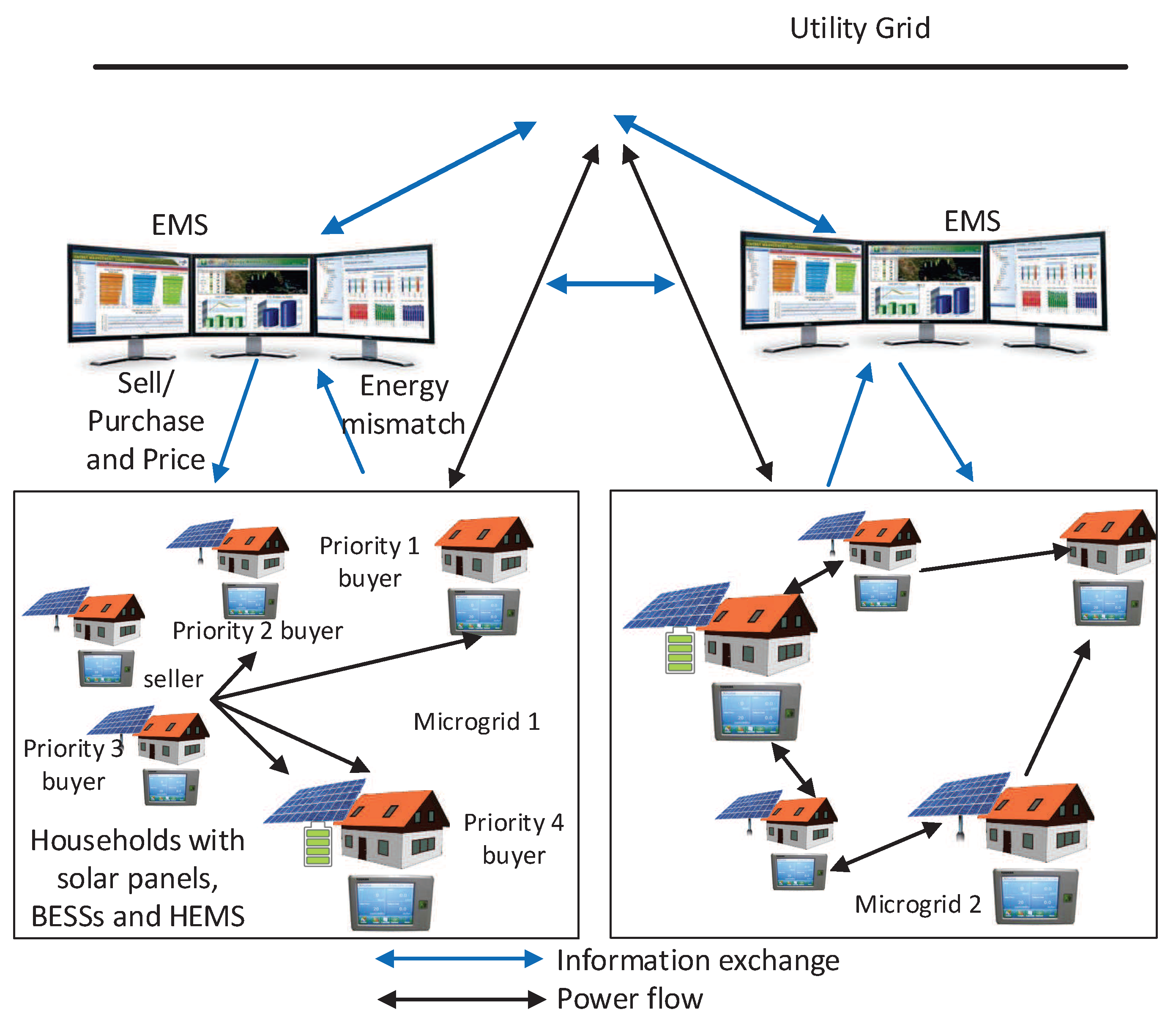
These priorities are set on the basis that buyers who need to satisfy their essential load demand (e.g., lighting, stove) are given more priority than buyers who need energy for heating/cooling, washing machine or storage. Note that the approach presented in this paper will still be applicable for priorities set in different orders. The inter-microgrid energy trading will take place if there is any excess/demand after intra-microgrid energy trading. The system model for intra-microgrid and inter-microgrid energy trading is illustrated in Figure 1.

The set of buyers and the set of sellers in the ${\ell }^{th}$ microgrid at a certain time instant are denoted by ${\mathcal{U}}_{\ell }\subseteq {\mathcal{N}}_{\ell }$ and ${\mathcal{V}}_{\ell }\subseteq {\mathcal{N}}_2+{\mathcal{N}}_3$. The buyers and sellers are denoted by the indices $u_{\ell }\in [1,U_{\ell }]$ and $v_{\ell }\in [1,V_{\ell }]$, respectively. The buyers in priority class 1, 2, 3 and 4 are denoted by ${\mathcal{U}}_1$, ${\mathcal{U}}_2$, ${\mathcal{U}}_3$ and ${\mathcal{U}}_4$, respectively. The amount of energy sold by the $v_{\ell }^{th}$ seller is $X_{v_{\ell }}$ and the amount of energy purchased by the $u_{\ell }^{th}$ buyer is $Y_{u_{\ell }}$. The energy price for purchasing $X_{u_{\ell }}$ amount of energy from the $v_{\ell }^{th}$ seller is $p\left(X_{v_{\ell }}\right)$. That is, the price is considered to be a function of the amount of sold energy.

The capital investment from the $v_{\ell }^{th}$ seller is $C_{v_{\ell }}$ and the seller expects to recover $m\%$ of the investment from profit earned by energy trading at a certain time instant. The feed-in tariff and the utility rates are denoted by $P_{feed-in}$ and $P_{util}$, respectively. The $u_{\ell }^{th}$ buyer expects to save $q\%$ of the energy bill that it would have paid to the utility if energy trading option was not available. Similarly, the energy purchased by the ${\ell }^{th}$ microgrid (when it has energy deficit) from the ${{\ell }^{\prime }}^{th}$ microgrid (when it has energy excess) is denoted by $E_{{\ell }^{\prime },\ell }$. The price for purchasing $E_{{\ell }^{\prime },\ell }$ amount of energy through inter-microgrid energy trading is $p_{inter}\left(E_{{\ell }^{\prime },\ell }\right)$.

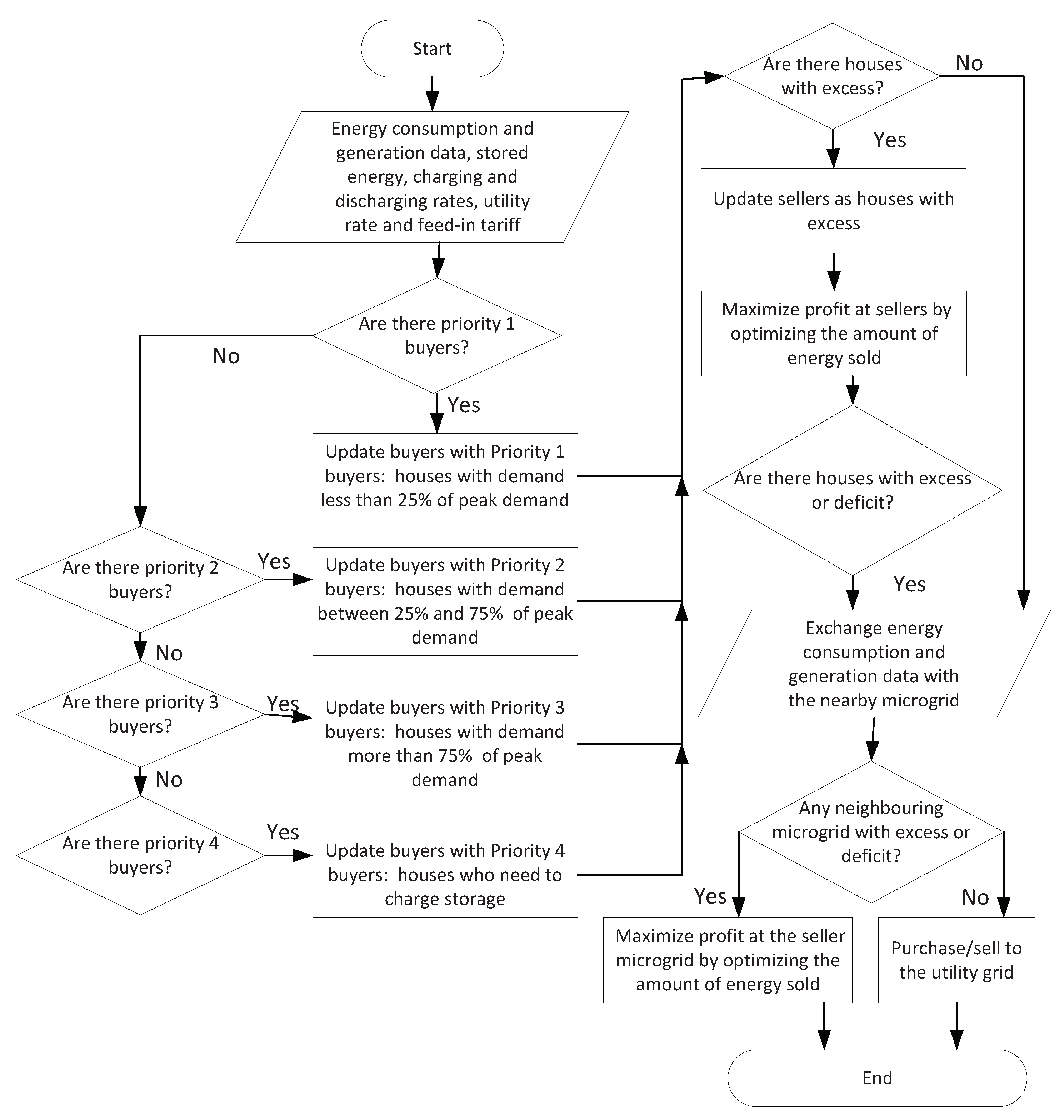
The energy trading mechanism takes place in the following manner. At a certain time instant, each house with energy excess/deficit reports to the central EMS of the microgrid and based on that, the EMS identifies the sellers and buyers. In addition, it also identifies the buyers in priority classes 1, 2, 3 and 4. If the number of sellers $V_{ell}$ and the number of buyers in priority class 1 $U_1$ are both non-zero, then the EMS performs the first stage of optimization and allocates an optimum amount of energy from the sellers to meet all or some part of the demand at the buyers in ${\mathcal{U}}_1$. Then the EMS recalculates the excess energy available at the sellers and updates the set ${\mathcal{V}}_{\ell }$. If the number of sellers and the number of buyers in ${\mathcal{U}}_2$ are both non-zero, then the EMS performs the second stage of optimization. In a similar manner, the EMS performs the third and fourth stage of optimization based on the availability of buyers and sellers for intra-microgrid energy trading.

After the fourth stage, if the number of buyers or sellers is still non-zero, the EMS at the ${\ell }^{th}$ microgrid notifies this information to the nearby microgrids. The microgrids that have energy excess/deficit responds to the ${\ell }^{th}$ microgrid and then the ${\ell }^{th}$ microgrid performs energy trading with the nearest buyer/seller. The seller optimizes the amount of energy to be sold and notifies the buyer. The remaining energy excess/deficit in any of the L microgrids are then balanced by the main power grid. The aforementioned process is illustrated in Figure 2.

3. Optimization Problem Formulation

In this section, the optimization problem is formulated for different stages of intra-microgrid energy trading, as well as inter-microgrid energy trading. For both the intra-microgrid and inter-microgrid energy trading, the sellers aim to maximize their profit while the supply-demand balance is maintained.

3.1. Intra-Microgrid Trading: Stage 1

In this stage, the sellers sell optimized amount of energy to the buyers in ${\mathcal{U}}_1$. For this, the central EMS of the ${\ell }^{th}$ microgrid solves the following optimization problem:

$$\begin{array}{c}\hfill \underset{X_{v_{\ell }},p\left(X_{v_{\ell }}\right)S_{v_{\ell }}^{\prime },S_{u_{\ell }}^{\prime },u_{\ell }\in [1,U_1],v_{\ell }\in [1,V_{\ell }]}{max}p\left(X_{v_{\ell }}\right)X_{v_{\ell }}\end{array}$$

(1)

$$\begin{array}{c}\hfill X_{v_{\ell }}\le G_{v_{\ell }}-D_{v_{\ell }}\forall v_{\ell }\in {\mathcal{N}}_2\cap {\mathcal{V}}_{\ell }\end{array}$$

(2)

$$\begin{array}{c}\hfill X_{v_{\ell }}\le G_{v_{\ell }}+\beta (S_{v_{\ell }}-S_{v_{\ell }}^{\prime })-D_{v_{\ell }}\forall v_{\ell }\in {\mathcal{N}}_3\cap {\mathcal{V}}_{\ell }\end{array}$$

(3)

$$\begin{array}{c}\hfill \sum _{v_{\ell }=1}^{V_{\ell }}{X}_{v_{\ell }}\le \sum _{u_{\ell }=1,u_{\ell }\in {\mathcal{U}}_1\cap {\mathcal{N}}_1}^{U_{\ell }}{D}_{u_{\ell }}+\sum _{u_{\ell }=1,u_{\ell }\in {\mathcal{U}}_1\cap {\mathcal{N}}_2}^{U_{\ell }}(D_{u_{\ell }}-G_{u_{\ell }})\\ \hfill +\sum _{u_{\ell }=1}^{U_{\ell },u_{\ell }\in {\mathcal{U}}_1\cap {\mathcal{N}}_3}(D_{u_{\ell }}-G_{u_{\ell }}+\frac{S_{u_{\ell }}^{\prime }-S_{u_{\ell }}}{\alpha })\end{array}$$

(4)

$$\begin{array}{c}\hfill P_{feed-in}\le p\left(X_{v_{\ell }}\right)\le P_{util}\forall v_{\ell }\in {\mathcal{V}}_{\ell }\end{array}$$

(5)

$$\begin{array}{c}\hfill p\left(X_{v_{\ell }}\right)X_{v_{\ell }}\ge \frac{m}{100}\times C_{v_{\ell }}\forall v_{\ell }\in {\mathcal{V}}_{\ell }\end{array}$$

(6)

$$\begin{array}{c}\hfill p\left(Y_{u_{\ell }}\right)Y_{u_{\ell }}\le (1-\frac{q}{100})\times P_{util}{Y}_{u_{\ell }}\forall u_{\ell }\in {\mathcal{U}}_1\end{array}$$

(7)

$$\begin{array}{c}\hfill S_{min}\le S_{\ell }^{\prime }\le S_{max}\forall \ell \in \mathcal{L}\end{array}$$

(8)

$$\begin{array}{c}\hfill S_{v_{\ell }}-S_{v_{\ell }}^{\prime }=r_{dch}{S}_{max}\forall v_{\ell }\in {\mathcal{V}}_{\ell }\end{array}$$

(9)

$$\begin{array}{c}\hfill S_{u_{\ell }}^{\prime }-S_{u_{\ell }}=r_{ch}{S}_{max}\forall u_{\ell }\in {\mathcal{U}}_1\cap {\mathcal{N}}_3\end{array}$$

(10)

where the objective function in Equation (1) indicates that the EMS is maximizing the profit at each seller when they sell energy to buyers in ${\mathcal{U}}_1$ and optimizes the amount of energy to be sold by each seller. Constraints Equations (2) and (3) ensure that the amount of sold energy is limited by the available energy at the seller. Here Equation (2) applies for houses with solar panels but no storage and Equation (3) applies for houses with both solar panels and storages. The constraint Equation (3) can be re-arranged in the following manner so that the variables are on the left hand side:

$$X_{v_{\ell }}+\beta S_{v_{\ell }}^{\prime }\le G_{v_{\ell }}+\beta S_{v_{\ell }}-D_{v_{\ell }}\forall v_{\ell }\in {\mathcal{N}}_3\cap {\mathcal{V}}_{\ell }$$

(11)

The constraint Equation (4) ensures that the amount of sold energy is limited by the total demand of the priority 1 buyers. Note that the first term in the right hand side represents buyers without solar panels or storage, the second term represents the buyers with solar panels but no storage and the third term represents the buyers with both solar panels and storage. This constraint can be re-arranged as follows:

$$\sum _{v_{\ell }=1}^{V_{\ell }}{X}_{v_{\ell }}-\frac{S_{u_{\ell }}^{\prime }}{\alpha }\le \sum _{u_{\ell }=1,u_{\ell }\in {\mathcal{U}}_1\cap {\mathcal{N}}_1}^{U_{\ell }}{D}_{u_{\ell }}+\sum _{u_{\ell }=1,u_{\ell }\in {\mathcal{U}}_1\cap {\mathcal{N}}_2}^{U_{\ell }}(D_{u_{\ell }}-G_{u_{\ell }})+\sum _{u_{\ell }=1}^{U_{\ell },u_{\ell }\in {\mathcal{U}}_1\cap {\mathcal{N}}_3}(D_{u_{\ell }}-G_{u_{\ell }}-\frac{S_{u_{\ell }}}{\alpha })$$

(12)

The constraint Equation (5) limits the price within the feed-in tariff and utility rate. The price needs to be higher than the feed-in tariff to attract the sellers for trading within the microgrid. The price needs to be lower than the utility rate to attract the buyers in the microgrid. The constraint Equation (6) ensures that the profit earned by the seller can recover at least $m\%$ of the capital cost incurred by the houses with solar panels and with/without storages. To allow the buyers save at least $q\%$ of the electricity bill that they would have to pay if the same amount of energy is purchased from the utility, constraint Equation (7) is applied. It is considered that the $u_{\ell }^{th}$ buyer is allocated ${\gamma }_{u_{\ell }}$ fraction of the sold energy, where ${\gamma }_{u_{\ell }}=\frac{D_{u_{\ell }}}{{\sum }_{i=1}^{U_1}{D}_i}$. This is chosen to allocate the buyers with the amount of energy in proportion to their energy demand at that time instant. Thus, the constraint Equation (7) can be simplified as:

$$p({\gamma }_{u_{\ell }}\sum _{v_{\ell }=1}^{V_{\ell }}{X}_{v_{\ell }})\le (1-\frac{q}{100})\times P_{util}\forall u_{\ell }\in {\mathcal{U}}_1$$

(13)

The constraint Equation (8) limits the stored energy between $S_{min}$ and $S_{max}$. To ensure that the storages are charged and discharged at the corresponding rates, constraints Equations (10) and (9) are applied.

3.2. Intra-Microgrid Trading: Stage 2

After solving the optimization problem in stage 1, the EMS re-calculates the available energy at the sellers in stage 1. Then it updates the number of sellers based on the houses that have energy excess. Next, the EMS of the ${\ell }^{th}$ microgrid solves the optimization problem as in Equation (1) where $u_{\ell }\in [1,U_2]$ and ${\gamma }_{u_{\ell }}=\frac{D_{u_{\ell }}}{{\sum }_{i=1}^{U_2}{D}_i}$. Also, the right hand side of the constraints in Equations (2), (11) and Equation (12) are updated by subtracting the amount of sold energy by the seller in stage 1. Then the EMS obtains the optimum amount of energy to be sold by the sellers in Stage 2 to the buyers in ${\mathcal{U}}_2$.

3.3. Intra-Microgrid Trading: Stage 3

Once the optimization problem in stage 2 is solved, the EMS updates the number of sellers based on the houses that have energy excess after stage 2. Next, the EMS of the ${\ell }^{th}$ microgrid solves the optimization problem as in Equation (1) where $u_{\ell }\in [1,U_3]$ and ${\gamma }_{u_{\ell }}=\frac{D_{u_{\ell }}}{{\sum }_{i=1}^{U_3}{D}_i}$. Moreover, the constraints in Equation (2), Equations (11) and (12) are updated by subtracting the amount of sold energy by the seller in stage 1 and 2 from the right hand side. Thus, the EMS optimizes the amount of energy sold by the sellers in Stage 3 to the buyers in ${\mathcal{U}}_3$.

3.4. Intra-Microgrid Trading: Stage 4

After stage 3 optimization, the EMS calculates the number of houses that have energy excess and updates the number of sellers. Next, the EMS optimizes the amount of sold energy as in Equation (1) where $u_{\ell }\in [1,U_4]$ and ${\gamma }_{u_{\ell }}=\frac{S_{u_{\ell }}+r_{ch}{S}_{max}}{{\sum }_{i=1}^{U_4}{S}_i+r_{ch}{S}_{max}}$. Then the amount of sold energy by the seller in stage 1, 2 and 3 are subtracted from the right hand side of the constraints in Equations (2) and (11). The constraint Equation (12) is updated by removing the first two terms (i.e., the buyers from ${\mathcal{N}}_1$ and ${\mathcal{N}}_2$) from the right hand side and then subtracting the amount of sold energy in the first three stages. Finally the EMS optimizes the amount of energy sold by the sellers in Stage 4 to the buyers in ${\mathcal{U}}_4$.

For intra-microgrid energy trading, the price set by the $v_{\ell }^{th}$ seller is represented by:

$$p\left(X_{v_{\ell }}\right)=a_{v_{\ell }}{X}_{v_{\ell }}+b_{v_{\ell }}$$

(14)

where the coefficients $a_{v_{\ell }}$ and $b_{v_{\ell }}$ are optimized to achieve maximum profit at the $v_{\ell }^{th}$ seller. Such linear function is widely adopted in the literature when considering energy trading applications [36]. Substituting the function into the optimization problem defined by Equations (1)–(10), the original problem can be re-written as:

$$\begin{array}{c}\hfill \underset{X_{v_{\ell }},a_{v_{\ell }},b_{v_{\ell }},S_{v_{\ell }}^{\prime },S_{u_{\ell }}^{\prime },u_{\ell }\in [1,U_1],v_{\ell }\in [1,V_{\ell }]}{max}{a}_{v_{\ell }}{X}_{v_{\ell }}^2+b_{v_{\ell }}{X}_{v_{\ell }}\end{array}$$

(15)

constraints Equations (2), (11), (12)

$$\begin{array}{c}\hfill P_{feed-in}\le a_{v_{\ell }}{X}_{v_{\ell }}+b_{v_{\ell }}\le P_{util}\forall v_{\ell }\in {\mathcal{V}}_{\ell }\end{array}$$

(16)

$$\begin{array}{c}\hfill a_{v_{\ell }}{X}_{v_{\ell }}^2+b{X}_{v_{\ell }}\ge \frac{m}{100}\times C_{v_{\ell }}\forall v_{\ell }\in {\mathcal{V}}_{\ell }\end{array}$$

(17)

$$\begin{array}{c}\hfill \sum _{v_{\ell }=1}^{V_{\ell }}{a}_{v_{\ell }}{\gamma }_{u_{\ell }}{X}_{v_{\ell }}+b_{v_{\ell }}\le (1-\frac{q}{100})\times P_{util}\forall u_{\ell }\in {\mathcal{U}}_1\end{array}$$

(18)

constraints Equations (8)–(10).

The optimization problem in Equation (15) can be represented as a quadratic programming problem with quadratic constraints and can be solved using existing solver packages like BMIBNB [37] employing branch and bound method for non-convex problems.

$$\begin{array}{c}\hfill Specialcase:a_{v_{\ell }}=0\end{array}$$

In this case, the price function for the $v_{\ell }^{th}$ seller simplifies to $b_{v_{\ell }}$. This case resembles to real time pricing, which is independent of the amount of energy sold. Here, the optimization problem defined in Equation (15) can be re-written as:

$$\begin{array}{cc}\hfill \underset{X_{v_{\ell }},b_{v_{\ell }},S_{v_{\ell }}^{\prime },S_{u_{\ell }}^{\prime },u_{\ell }\in [1,U_1],v_{\ell }\in [1,V_{\ell }]}{max}& b_{v_{\ell }}{X}_{v_{\ell }}\hfill \end{array}$$

(19)

Similarly, the constraints Equations (16)–(18) can be re-written as:

$$\begin{array}{c}\hfill P_{feed-in}\le b_{v_{\ell }}\le P_{util}\forall v_{\ell }\in {\mathcal{V}}_{\ell }\end{array}$$

(20)

$$\begin{array}{c}\hfill b{X}_{v_{\ell }}\ge \frac{m}{100}\times C_{v_{\ell }}\forall v_{\ell }\in {\mathcal{V}}_{\ell }\end{array}$$

(21)

$$\begin{array}{c}\hfill \sum _{v_{\ell }=1}^{V_{\ell }}{b}_{v_{\ell }}\le (1-\frac{q}{100})\times P_{util}\forall u_{\ell }\in {\mathcal{U}}_1\end{array}$$

(22)

The optimal values of $b_{v_{\ell }}$ can be obtained by solving the aforementioned optimization problem. The optimal values for different time instants can be averaged to calculate a flat rate or they can be averaged over the peak, off-peak and shoulder usage periods separately to calculate the different price levels for time of use tariff structure.

3.5. Inter-Microgrid Energy Trading

Once the intra-microgrid energy trading is complete in the ${\ell }^{th}$ microgrid and there is excess energy or deficit, the EMS of the ${\ell }^{th}$ microgrid performs inter-microgrid energy trading with the ${{\ell }^{\prime }}^{th}$ microgrid. The ${{\ell }^{\prime }}^{th}$ microgrid is the closest microgrid from the ${\ell }^{th}$ microgrid that has the ability to reduce the mismatch between supply and demand at the ${\ell }^{th}$ microgrid. The optimization problem for inter-microgrid energy trading where ${\ell }^{th}$ microgrid is a seller and the ${{\ell }^{\prime }}^{th}$ microgrid is a buyer can be formulated as:

$$\begin{array}{c}\hfill \underset{E_{\ell ,{\ell }^{\prime }},p_{inter}\left(E_{\ell ,{\ell }^{\prime }}\right)S_{n_{\ell }}^{\prime },S_{n_{{\ell }^{\prime }}}^{\prime },n_{\ell }\in [1,N_{\ell }]}{max}{p}_{inter}\left(E_{\ell ,{\ell }^{\prime }}\right)E_{\ell ,{\ell }^{\prime }}\end{array}$$

(23)

$$\begin{array}{c}\hfill E_{\ell ,{\ell }^{\prime }}\le \sum _{n_{\ell }=1}^{N_2}{G}_{n_{\ell }}+\sum _{n_{\ell }=1}^{N_3}{G}_{n_{\ell }}+\sum _{n_{\ell }=1}^{N_3}\beta (S_{n_{\ell }}-S_{n_{\ell }}^{\prime })-\sum _{n_{\ell }=1}^{N_1}{D}_{n_{\ell }}-\sum _{n_{\ell }=1}^{N_2}{D}_{n_{\ell }}-\sum _{n_{\ell }=1}^{N_3}{D}_{n_{\ell }}\end{array}$$

(24)

$$\begin{array}{c}\hfill E_{\ell ,{\ell }^{\prime }}\le \sum _{n_{{\ell }^{\prime }}=1}^{N_2}{G}_{n_{{\ell }^{\prime }}}+\sum _{n_{{\ell }^{\prime }}=1}^{N_3}{G}_{n_{{\ell }^{\prime }}}+\sum _{n_{{\ell }^{\prime }}=1}^{N_3}\frac{S_{n_{{\ell }^{\prime }}}^{\prime }-S_{n_{{\ell }^{\prime }}}}{\alpha }-\sum _{n_{{\ell }^{\prime }}=1}^{N_1}{D}_{n_{{\ell }^{\prime }}}-\sum _{n_{{\ell }^{\prime }}=1}^{N_2}{D}_{n_{{\ell }^{\prime }}}-\sum _{n_{{\ell }^{\prime }}=1}^{N_3}{D}_{n_{{\ell }^{\prime }}}\end{array}$$

(25)

$$\begin{array}{c}\hfill P_{feed-in}\le p_{inter}\left(E_{\ell ,{\ell }^{\prime }}\right)\le P_{util}\end{array}$$

(26)

$$\begin{array}{c}\hfill S_{min}\le S_{n_{\ell }}^{\prime },S_{n_{\ell }^{\prime }}^{\prime }\le S_{max}\forall n_{\ell }\in {\mathcal{N}}_{\ell }\end{array}$$

(27)

$$\begin{array}{c}\hfill S_{n_{\ell }}-S_{n_{\ell }}^{\prime }=r_{dch}{S}_{max}\forall n_{\ell }\in {\mathcal{N}}_3\end{array}$$

(28)

$$\begin{array}{c}\hfill S_{n_{{\ell }^{\prime }}}^{\prime }-S_{n_{{\ell }^{\prime }}}=r_{ch}{S}_{max}\forall n_{{\ell }^{\prime }}\in {\mathcal{N}}_3\end{array}$$

(29)

where Equation (23) represents the objective function which obtains the optimum amount of energy to be sold so that the profit at the ${\ell }^{th}$ seller can be maximized. The constraints Equations (24) and (25) limit the amount of energy sold by the available energy at the seller microgrid and the demand at the buyer microgrid. The price for inter-microgrid energy trading is limited between feed-in tariff and utility rate according to the constraint in Equation (26). The constraint Equation (27) indicates that the stored energy at all the houses in the ${\ell }^{th}$ and the ${{\ell }^{\prime }}^{th}$ microgrid is limited between the minimum and maximum values.

Similar to intra-microgrid energy trading, the pricing function considered for inter-microgrid energy trading is a linear function of the amount of energy sold. That is,

$$p\left(E_{\ell ,{\ell }^{\prime }}\right)=a_{\ell ,{\ell }^{\prime }}{E}_{\ell ,{\ell }^{\prime }}+b_{\ell ,{\ell }^{\prime }}$$

(30)

where $a_{\ell ,{\ell }^{\prime }}$ and $b_{\ell ,{\ell }^{\prime }}$ are the coefficients optimized by the ${\ell }^{th}$ microgrid when it sells excess energy to the ${{\ell }^{\prime }}^{th}$ microgrid. The optimization problem for inter-microgrid energy trading can be re-written after substituting the pricing function in the following manner:

$$\begin{array}{c}\hfill \underset{E_{\ell ,{\ell }^{\prime }},a_{\ell ,{\ell }^{\prime }},b_{\ell ,{\ell }^{\prime }}{S}_{n_{\ell }}^{\prime },S_{n_{{\ell }^{\prime }}}^{\prime },n_{\ell }\in [1,N_{\ell }]}{max}{a}_{\ell ,{\ell }^{\prime }}{E}_{\ell ,{\ell }^{\prime }}^2+b{E}_{\ell ,{\ell }^{\prime }}\end{array}$$

(31)

constraints Equations (24), (25)

$$\begin{array}{c}\hfill P_{feed-in}\le a_{\ell ,{\ell }^{\prime }}{E}_{\ell ,{\ell }^{\prime }}+b_{\ell ,{\ell }^{\prime }}\le P_{util}\end{array}$$

(32)

constraints Equations (27)–(29).

The optimization problem in Equation (15) can be represented as a quadratic programming problem with quadratic constraints and can be solved using existing solver packages like BMIBNB [37] employing the branch and bound method for non-convex problems. Similar to intra-microgrid energy trading, the pricing function coefficient $b_{\ell ,{\ell }^{\prime }}$ can be optimized for real time pricing, flat rate pricing and time of use pricing structures when $a_{\ell ,{\ell }^{\prime }}=0$.

4. Numerical Results

In this section, the impact of optimum energy trading on the energy supply/demand balance and profit earned by the sellers are evaluated numerically and compared with the no energy trading scenarios, as well as a different pricing structure.

4.1. Materials and Data

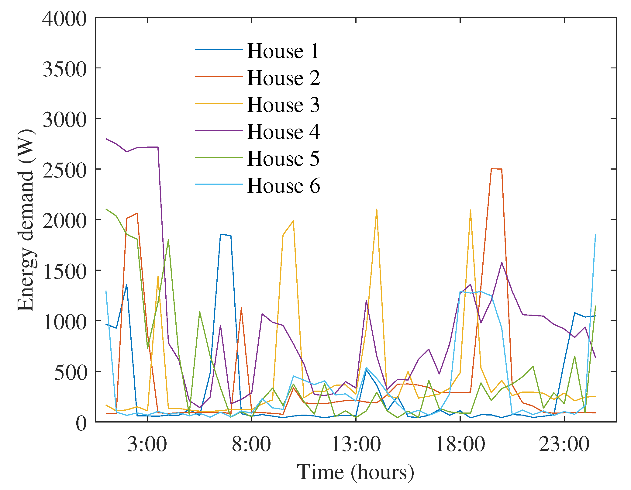
The author has considered $L=2$ microgrids where each microgrid has $N_{\ell }$ = 6 houses with $N_1=2$, $N_2=2$ and $N_3=2$. Among these six houses, House 1 and 2 are not equipped with solar panels or storages, House 3 and 4 are equipped with solar panels only and House 5 and 6 have both solar panels and storages. The installed capacity of the solar panels at Houses 3, 4, 5 and 6 are 2, 1.62, 3.78 and 2.16 kW, respectively. The storage capacity of the batteries at Houses 5 and 6 are 1.5 and 1 kW, respectively. The charging and discharging efficiencies are 0.7 and 0.5, respectively. The discharging and charging rates are 0.5 and 0.2, respectively. The utility rate and feed-in-tariff are considered as 30 cents/kWh and 5 cents/kWh, respectively. The capital investment at Houses 3, 4, 5 and 6 are $5000, $3000, $10,000 and $8000, respectively. Here, $q=0.2$ and $m=0.1$ has been considered. The energy generation and consumption data is obtained for each 30 min interval from 12:30 a.m. on 1 July 2012 to 12:00 a.m. on 2 July 2012 for NSW, Australia from [38]. The demand profiles of the 6 houses in microgrid 1 are shown in Figure 3. Note that the optimization problem is solved only for the time intervals when the number of sellers and buyers are non-zero, typically each 30 min interval from 10:30 a.m. to 4:30 p.m. The solution algorithm is implemented in MATLAB 2018b using the ‘bmibnb’ solver from ‘YALMIP’ package [37]. The overall computation time is 25 s for an Intel Core i5-6300U CPU with 2.4 GHz processing speed.

4.2. Energy Mismatch with Optimum Energy Trading

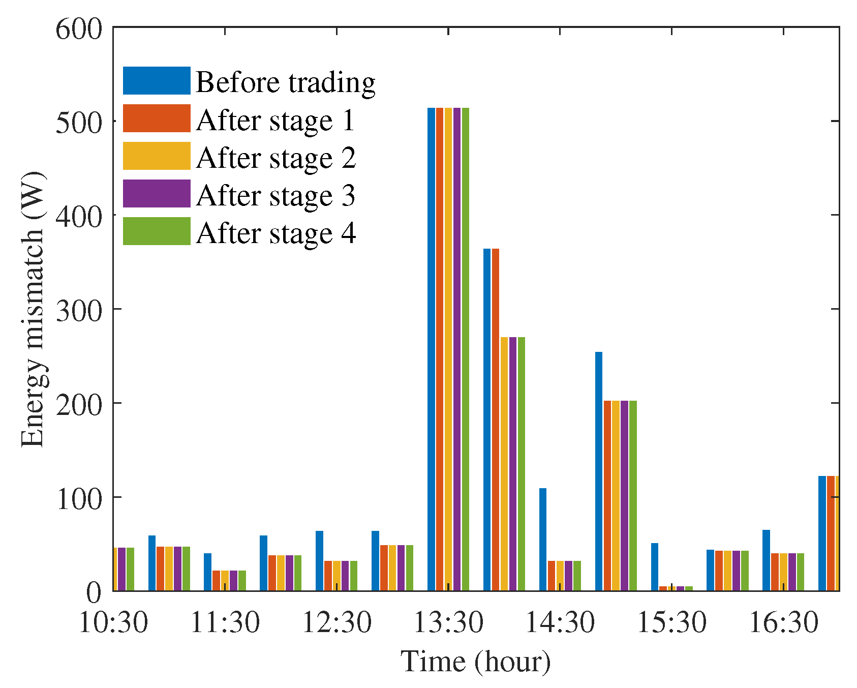
Figure 4a–e demonstrate the energy mismatch before and after energy trading when multiple stages are present, corresponding to different priorities. Here, positive energy mismatch represents energy deficit, whereas negative energy mismatch denotes energy excess. Comparing Figure 4e and Figure 4a, it can be seen that after stage 1 (when only houses with demand less than $25\%$ of the peak demand are considered as buyers), the energy deficit decreases for Houses 1 and 3 during hours 10:00 a.m.–1:00 p.m., when there is enough solar generation. Similarly, the energy excess at Houses 5 and 6 also decreases, as this energy is used by other houses. Comparing Figure 4a and Figure 4b, it can be seen that the energy deficit at House 2 further decreases during 12.30 p.m.–3.00 p.m. (as indicated in the zoomed sections). From Figure 4b,c, the energy deficit at House 6 decreases during 10.00 a.m.– 12.30 p.m. Also, the energy excess at house 4 decreases during 11.00–11.30 a.m. as it is being used by other houses (as indicated by the zoomed sections). Finally, from Figure 4d, it can be seen that the excess energy at House 4 is completely utilized by Houses 5 and 6 to charge their storages. So, Houses 5 and 6 now have stored energy to utilize in the following time instants, as well as to sell to the other microgrid.

Figure 5 shows the energy mismatch at house 1 before energy trading and after each stage of energy trading. It can be seen that the energy mismatch decreases mostly after stage 1, because house 1 has priority 1 demand (demand less than 25% of the peak demand) for most of the times during 10:30 a.m. to 4:30 p.m. However, at 2 p.m., the energy mismatch decreases after stage 2, indicating that house 1 has a priority 2 demand (demand between 25–50% of the peak demand). The energy mismatch at 1:30 p.m. did not decrease due to insufficient generation to meet house 1’s priority 2 demand. The available generation is utilized by other houses who had priority 1 demand.

Figure 6 shows how the energy mismatch at different houses change when no priorities are considered for allocating the energy from the sellers and, as a result, energy trading optimization problem is solved in a single stage. Comparing Figure 6 with Figure 4d, it can be seen that the energy mismatch can be minimized to zero for more houses when priorities are considered. For example, the energy deficit at House 3 and energy excess at House 4 is less in Figure 4d during 10–10.30 a.m. Moreover, the energy excess at houses 5 and 6 decrease as well when priorities are considered. Since the proposed approach prioritizes buyers with lower energy demand, this might lead to higher energy mismatch at buyers with higher energy demand compared to the single stage energy trading optimization (with no priorities) at certain hours when the generation is not sufficient.

4.3. Profit Earned with Different Pricing Structures

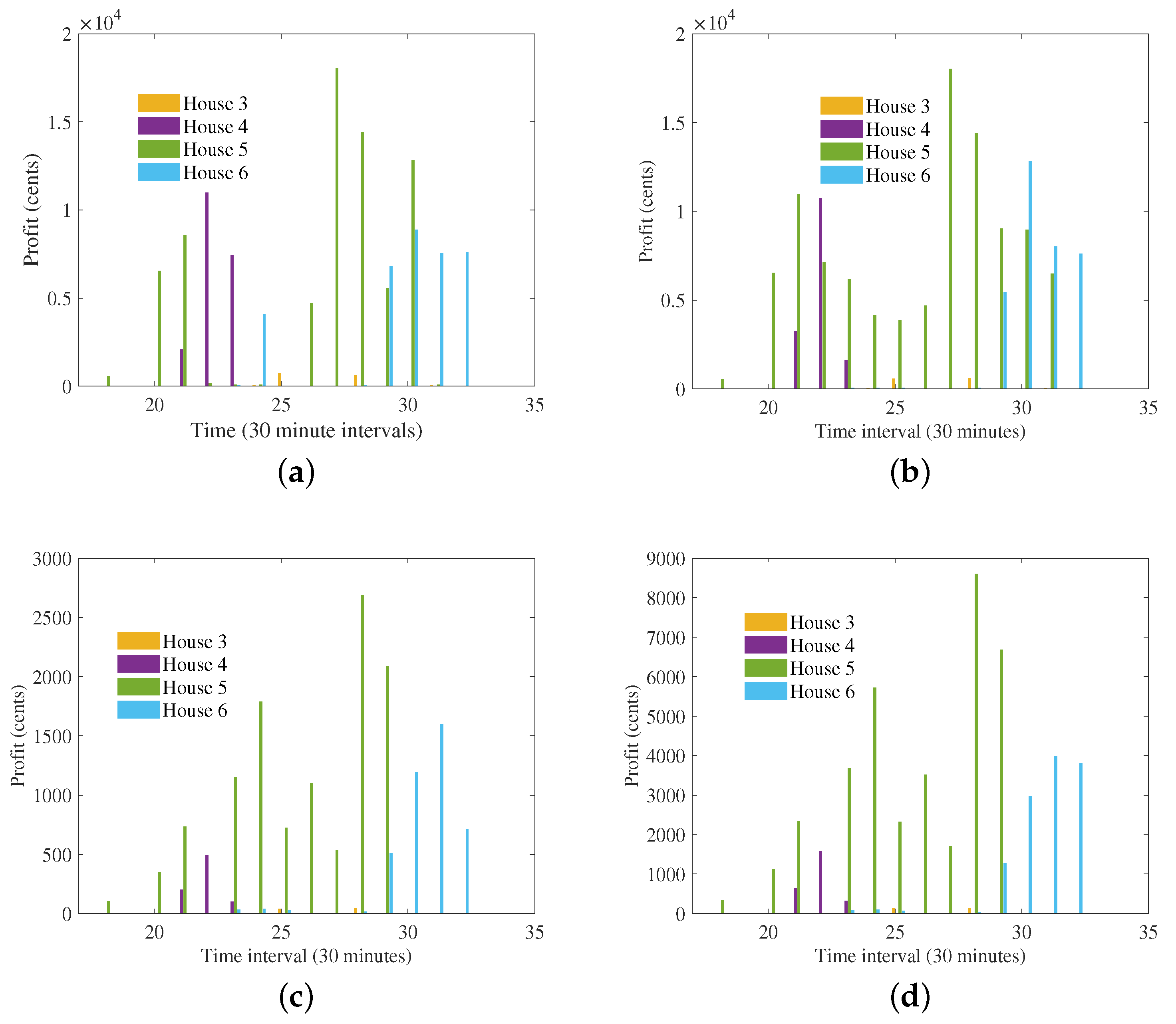
Figure 7a–d demonstrate the maximum profits earned by the sellers during different time intervals of the day when different pricing structures are considered. Here the results are shown from 9 a.m.–5 p.m., as the solar energy generation occupy this time period primarily. Figure 7a plots the solution of Equation (15), whereas Figure 7b represents the solution of Equation (19). The results in Figure 7c is based on the solution of Equation (19) but the optimum price vector is averaged over the day to obtain a flat pricing. Similarly, for Figure 7d is plotted by averaging the pricing for 9 a.m.– 4 p.m. for off-peak and 4 p.m.–5p.m. for peak rate. It can be seen that House 5 earns the maximum profit among all houses and for more hours in the day, since it has larger solar panel and storage. House 6 earns profits mostly during 2.30–4.00 p.m. From the aforementioned figures, it is clear that the maximum profit earned with pricing as a function of energy is larger than the profit earned with other pricing structure. The maximum profit earned at House 2 with both the proposed and real-time pricing structures are the same. However, Houses 4 and 6 earn more profit with the proposed pricing structure during 11.30 a.m. and 12.00 p.m. With flat rate and time of use pricing, the profits earned are significantly less than the proposed and real time pricing structures.

4.4. Impact of Feed-in-Tariff and Energy Savings Threshold at the Buyers

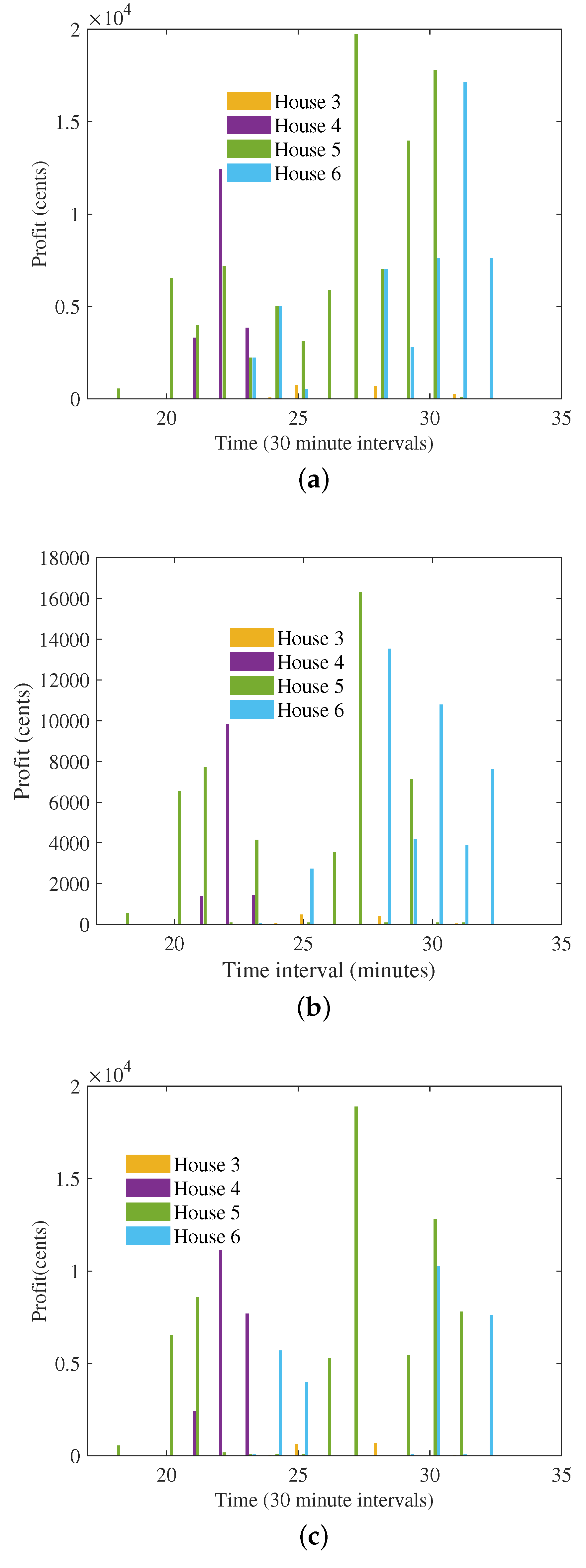
Figure 8a demonstrates the profit earned by the sellers when feed-in tariff is selected as 11 cents. This changes the constraint in Equation (16) in such a way that the resulting pricing will need to exceed a larger threshold. As a result, the profit earned by the sellers increases when $P_f$ is set to a larger value, which can be seen by comparing Figure 7a and Figure 8a. Figure 8b,c show the impact of different values of q on the maximum profit earned by the sellers. A higher value of q represents a greater savings for the buyer, indicating the energy price will be lower. This results into a lower profit for the sellers. As a result, it can be seen from Figure 8b and Figure 7a that the profit earned by sellers decreases when q increases from 0.2 to 0.4. On the other hand, comparing Figure 7a and Figure 8b, it can be seen that the profits increase slightly when q decreases from 0.2 to 0.1.

4.5. Inter-Microgrid Energy Trading

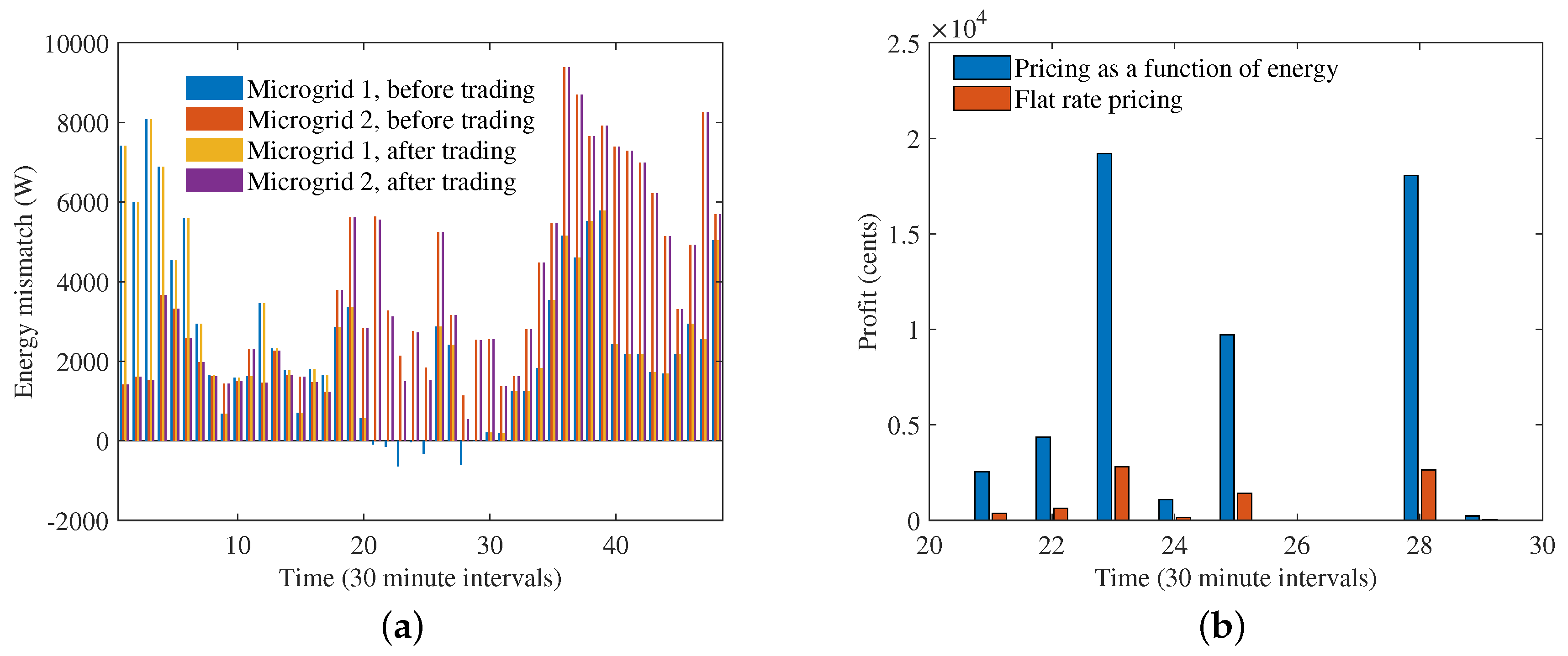
Figure 9a shows the energy mismatch before and after inter-microgrid energy trading at the two microgrids. It can be seen that the energy mismatch at both microgrids decreases between 10.00 a.m.–2.30 p.m. For microgrid 1, the energy excess is completely minimized, whereas for microgrid 2, the energy deficit is reduced during this time period. Figure 9b shows the profit earned by the seller microgrid with the proposed pricing structure as well as flat rate pricing. Note that the real time pricing structure results into same profit as the proposed pricing structure. Thus, it can be concluded that the amount of profits increase significantly when variable hourly pricing is considered.

5. Conclusions

In this paper, research questions on how to maximize profits for local energy trading within a microgrid, as well as among multiple microgrids, are considered. Moreover, the research also considered how energy can be allocated to different priority groups, while maximizing profit for the sellers. In addition, the proposed pricing scheme is compared with existing schemes in terms of profit maximization for the sellers. To address the aforementioned research questions, a pricing scheme was designed as a linear function of the amount of energy sold and the pricing was optimized to achieve maximum profits for the sellers. It has been observed that the proposed approach can reduce energy mismatch at the participants more than that achieved without considering priority groups, under similar generation and demand characteristics. The optimum pricing function is shown to increase the profits for the sellers compared to the flat rate and ToU pricing schemes. The limitations of the proposed scheme are the requirements of a central controller/aggregator to compute the optimization outcomes and the assumption of the availability of accurate information about energy mismatch at the participants. Thus, future work will be based on optimizing the pricing signal for decentralized energy trading operations and investigating the impact of communication impairments on the profit obtained by participants in local energy trading.

References

- Deng, R.; Yang, Z.; Chow, M.; Chen, J. A survey on demand response in smart grids: Mathematical models and approaches. IEEE Trans. Ind. Inform. 2015, 11, 570–582. [Google Scholar] [CrossRef]
- Tronchina, L.; Manfrenb, M.; Nastasic, B. Energy efficiency, demand side management and energy storage technologies—A critical analysis of possible paths of integration in the built environment. Renew. Sustain. Energy Rev. 2018, 95, 341–353. [Google Scholar] [CrossRef]
- Reihani, E.; Motalleb, M.; Thornton, M.; Ghorbani, R. A novel approach using flexible scheduling and aggregation to optimize demand response in the developing interactive grid market architecture. Appl. Energy 2016, 183, 445–455. [Google Scholar] [CrossRef] [Green Version]
- Sousa, T.; Morais, H.; Vale, Z.; Faria, P.; Soares, J. Intelligent energy resource management considering vehicle-to-grid: A simulated annealing approach. IEEE Trans. Smart Grid 2012, 3, 535–542. [Google Scholar] [CrossRef]
- Doostizadeh, M.; Ghasemi, H. A day-ahead electricity pricing model based on smart metering and demand-side management. Energy 2012, 46, 221–230. [Google Scholar] [CrossRef]
- Mohsenian-Rad, A.; Leon-Garcia, A. Optimal residential load control with price prediction in real-time electricity pricing environments. IEEE Trans. Smart Grid 2010, 1, 120–133. [Google Scholar] [CrossRef]
- Qian, L.P.; Zhang, Y.J.A.; Huang, J.; Wu, Y. Demand response management via real-time electricity price control in smart grids. IEEE J. Sel. Areas Commun. 2013, 31, 1268–1280. [Google Scholar] [CrossRef]
- Yaghmaee, M.H.; Moghaddassian, M.; Leon-Garcia, A. Autonomous two-tier cloud-based demand side management approach with microgrid. IEEE Trans. Ind. Inform. 2017, 13, 1109–1120. [Google Scholar] [CrossRef]
- Tezde, E.I.; Okumus, H.I.; Savran, I. Two-Stage Energy Management of Multi-Smart Homes With Distributed Generation and Storage. Electronics 2019, 19, 512. [Google Scholar] [CrossRef]
- Muhsen, D.H.; Haider, H.T.; Al-Nidawi, Y.; Khatib, T. Optimal Home Energy Demand Management Based Multi-Criteria Decision Making Methods. Electronics 2019, 8, 524. [Google Scholar] [CrossRef]
- Long, C.; Wu, J.; Zhang, C.; Thomas, L.; Cheng, M.; Jenkins, N. Peer-to-peer energy trading in a community microgrid. In Proceedings of the 2017 IEEE Power & Energy Society General Meeting, Chicago, IL, USA, 16–20 July 2017; pp. 1–5. [Google Scholar]
- Joo, I.; Choi, D. Distributed optimization framework for energy management of multiple smart homes with distributed energy resources. IEEE Access 2017, 5, 15551–15560. [Google Scholar] [CrossRef]
- Long, C.; Wu, J.; Zhou, Y.; Jenkins, N. Peer-to-peer energy sharing through a two-stage aggregated battery control in a community microgrid. Appl. Energy 2018, 226, 261–276. [Google Scholar] [CrossRef]
- Hu, W.; Wang, P.; Gooi, H.B. Toward optimal energy management of microgrids via robust two-stage optimization. IEEE Trans. Smart Grid 2018, 9, 1161–1174. [Google Scholar] [CrossRef]
- Shamsi, P.; Xie, H.; Longe, A.; Joo, J. Economic dispatch for an agent-based community microgrid. IEEE Trans. Smart Grid 2016, 7, 2317–2324. [Google Scholar] [CrossRef]
- Sorin, E.; Bobo, L.; Pinson, P. Consensus-based approach to peer-to-peer electricity markets with product differentiation. IEEE Trans. Power Syst. 2019, 34, 994–1004. [Google Scholar] [CrossRef]
- Kang, J.; Yu, R.; Huang, X.; Maharjan, S.; Zhang, Y.; Hossain, E. Enabling localized peer-to-peer electricity trading among plug-in hybrid electric vehicles using consortium blockchains. IEEE Trans. Ind. Inform. 2017, 13, 3154–3164. [Google Scholar] [CrossRef]
- Kim, Y.-M.; Jung, D.; Chang, Y.; Choi, D.-H. Intelligent Micro Energy Grid in 5G Era: Platforms, Business Cases, Testbeds, and Next Generation Applications. Electronics 2019, 8, 468. [Google Scholar] [CrossRef]
- Zhou, Y.; Wu, J.; Long, C. Evaluation of peer-to-peer energy sharing mechanisms based on a multiagent simulation framework. Appl. Energy 2018, 222, 993–1022. [Google Scholar] [CrossRef]
- Morstyn, T.; McCulloch, M. Multi-class energy management for peer-to-peer energy trading driven by prosumer preferences. IEEE Trans. Power Syst. 2018, 1. [Google Scholar] [CrossRef]
- Opadokun, F.; Roy, T.K.; Akter, M.N.; Mahmud, M.A. Prioritizing customers for neighborhood energy sharing in residential microgrids with a transactive energy market. In Proceedings of the 2017 IEEE Power & Energy Society General Meeting, Chicago, IL, USA, 16–20 July 2017; pp. 1–5. [Google Scholar]
- Guerrero, J.; Chapman, A.C.; Verbič, G. Decentralized p2p energy trading under network constraints in a low-voltage network. IEEE Trans. Smart Grid 2018, 1. [Google Scholar] [CrossRef]
- Rahimiyan, M.; Baringo, L.; Conejo, A.J. Energy management of a cluster of interconnected price-responsive demands. IEEE Trans. Power Syst. 2014, 29, 645–655. [Google Scholar] [CrossRef]
- Gregoratti, D.; Matamoros, J. Distributed energy trading: The multiple-microgrid case. IEEE Trans. Ind. Electron. 2015, 62, 2551–2559. [Google Scholar] [CrossRef]
- Bahrami, S.; Amini, M.H.; Shafie-Khah, M.; Catalão, J.P.S. A decentralized renewable generation management and demand response in power distribution networks. IEEE Trans. Sustain. Energy 2018, 9, 1783–1797. [Google Scholar] [CrossRef]
- Islam, S.N.; Mahmud, M.; Oo, A. Impact of optimal false data injection attacks on local energy trading in a residential microgrid. ICT Express 2018, 4, 30–34. [Google Scholar] [CrossRef]
- Tushar, M.H.K.; Assi, C. Optimal energy management and marginal-cost electricity pricing in microgrid network. IEEE Trans. Ind. Inform. 2017, 13, 3286–3298. [Google Scholar] [CrossRef]
- Cali, U.; Çakir, O. Energy Policy Instruments for Distributed Ledger Technology Empowered Peer-to-Peer Local Energy Markets. IEEE Access 2019, 7, 82888–82900. [Google Scholar] [CrossRef]
- Vlachos, A.G.; Biskas, P.N. Balancing supply and demand under mixed pricing rules in multi-area electricity markets. IEEE Trans. Power Syst. 2011, 26, 1444–1453. [Google Scholar] [CrossRef]
- Lahon, R.; Gupta, C.P.; Fernandez, E. Priority-Based Scheduling of Energy Exchanges Between Cooperative Microgrids in Risk-Averse Environment. IEEE Syst. J. 2019. [Google Scholar] [CrossRef]
- Ruiz, C.; Conejo, A.J.; Gabriel, S.A. Pricing non-convexities in an electricity pool. IEEE Trans. Power Syst. 2012, 27, 1334–1342. [Google Scholar] [CrossRef]
- Hayes, B.; Melatti, I.; Mancini, T.; Prodanovic, M.; Tronci, E. Residential demand management using individualized demand aware price policies. IEEE Trans. Smart Grid 2017, 8, 1284–1294. [Google Scholar] [CrossRef]
- Sebastian, A.J.; Islam, S.N.; Mahmud, A.; Oo, A.M.T. Optimum Local Energy Trading considering Priorities in a Microgrid. In Proceedings of the 10th IEEE International Conference on Communications, Control, and Computing Technologies for Smart Grids (SmartGridComm 2019), Beijing, China, 21–24 October 2019. [Google Scholar]
- Ghosh, A.; Aggarwal, V. Control of charging of electric vehicles through menu-based pricing. IEEE Trans. Smart Grid 2018, 9, 5918–5929. [Google Scholar] [CrossRef]
- Hussain, A.; Bui, V.; Kim, H. Robust optimal operation of ac/dc hybrid microgrids under market price uncertainties. IEEE Access 2018, 6, 2654–2667. [Google Scholar] [CrossRef]
- Sanchez, S.; Molinas, M. Degree of influence of system states transition on the stability of a DC microgrid. IEEE Trans. Smart Grid 2014, 5, 2535–2542. [Google Scholar] [CrossRef]
- YALMIP. Bmibnb. Available online: https://yalmip.github.io/solver/bmibnb/ (accessed on 6 July 2019).
- Ausgrid. Solar Home Electricity Data. Available online: https://www.ausgrid.com.au/Industry/Innovation-and-research/Data-to-share/Solar-home-electricity-data (accessed on 6 July 2019).
Figure 1.
Local energy trading within a microgrid, as well as multiple microgrids. The microgrid 1 on the left hand side shows the different priority classes for buyers. Note that the priorities of the houses can be different based on the energy deficit and the thresholds. Each microgrid has a central EMS which coordinates the energy trading with another microgrid.
Figure 2.
Flowchart illustrating intra-microgrid and inter-microgrid energy trading optimization stages for different priority levels.
Figure 3.
Demand profile of the 6 houses under microgrid 1.
Figure 4.
Energy mismatch at the 6 houses in the microgrid before and after energy trading considering different priorities. (a) After stage 1, zoomed section indicates the energy mismatch at house 2 during 12:30–3:00 p.m.; (b) After stage 2, zoomed section indicates the energy mismatch at house 2 during 12:30–3:00 p.m.; (c) After stage 3, zoomed section indicates the energy mismatch at house 4 during 11:00–11:30 a.m.; (d) After stage 4, zoomed section indicates the energy mismatch at house 4 during 11:00–11:30 a.m.; (e) Without energy trading.
Figure 5.
Energy mismatch at house 1 in the microgrid with no energy trading and after different stages of energy trading.
Figure 6.
Energy mismatch at the 6 houses in the microgrid with energy trading when priorities are not considered.
Figure 7.
Hourly profit for the sellers in the microgrid considering different pricing structure. (a) Pricing as a function of energy; (b) Real time pricing; (c) Flat rate pricing; (d) Time of use pricing.
Figure 8.
Hourly profit for the sellers in the microgrid with different feed-in tariff and different thresholds for energy saving at the buyers. (a) cents; (b) ; (c) .
Figure 9.
Energy mismatch before and after inter-microgrid energy trading at the two microgrids and hourly profit. (a) Energy mismatch; (b) Profit.
© 2019 by the author. Licensee MDPI, Basel, Switzerland. This article is an open access article distributed under the terms and conditions of the Creative Commons Attribution (CC BY) license (http://creativecommons.org/licenses/by/4.0/).
Share and Cite
MDPI and ACS Style
Islam, S.N. A New Pricing Scheme for Intra-Microgrid and Inter-Microgrid Local Energy Trading. Electronics 2019, 8, 898. https://doi.org/10.3390/electronics8080898
AMA Style
Islam SN. A New Pricing Scheme for Intra-Microgrid and Inter-Microgrid Local Energy Trading. Electronics. 2019; 8(8):898. https://doi.org/10.3390/electronics8080898
Chicago/Turabian StyleIslam, Shama Naz. 2019. "A New Pricing Scheme for Intra-Microgrid and Inter-Microgrid Local Energy Trading" Electronics 8, no. 8: 898. https://doi.org/10.3390/electronics8080898
Note that from the first issue of 2016, this journal uses article numbers instead of page numbers. See further details here.