Partial Feedback Linearizing Model Predictive Controllers for Multiple Photovoltaic Units Connected to Grids through a Point of Common Coupling

Abstract

In this paper, partial feedback linearizing model predictive controllers are designed for grid-connected systems comprising multiple photovoltaic (PV) units where these units are connected through a point of common coupling (PCC). The proposed controllers are designed for voltage source inverters (VSIs) based on comprehensive dynamical models of grid-connected PV systems with the proposed topology. The proposed partial feedback linearization scheme decouples multiple PV units in the forms of several reduced-order subsystems and enables linear controller design through the linear continuous-time receding horizon model predictive control scheme. The proposed partial feedback linearization scheme also considers dynamic interactions among multiple PV units as external noises or disturbances and decouples these noises. This paper includes the noise decoupling capability of the partial feedback linearization for grid-connected PV systems with multiple PV units which are connected through a PCC. Simulation results clearly demonstrate the effectiveness of the proposed scheme under different operating conditions as compared to an existing proportional integral controller.

1. Introduction

Solar photovoltaic (PV) systems are considered as one of the most promising renewable energy sources (RESs) and the constructions of large-scale grid-connected solar PV systems are increasing around the world as these provide several benefits [1]. Most of these large-scale PV units are connected to a common bus which is often called as the point of common coupling (PCC) and then transmitted as well as distributed the power over large geographical areas. However, there are some technical issues due to the integration of solar PV systems and the power quality with desired tracking performances (i.e., voltage and frequency regulations) is considered as the major issue. Moreover, there are strong dynamic interactions as these PV units are located close to each other, i.e., their closed geographical locations within the network [2]. Therefore, it is essential to design controllers for such grid-connected PV systems that can tackle the aforementioned issues.

Dynamical models of grid-connected PV systems include the meaningful voltage-current relationships in order to represent the characteristics of the whole system and the dynamics of grid-connected PV systems abruptly changes with changes in atmospheric conditions [3,4]. Different maximum power point tracking (MPPT) techniques are employed to capture the maximum power from PV units under changing atmospheric conditions [5,6,7,8]. In this work, the main emphasis is given on the control of the voltage source inverter (VSI) instead of the maximum power point tracking. Since the dynamical models capture the useful characteristics, model-based control schemes are widely used to overcome the challenges in grid-connected PV systems [9,10,11].

Proportional integral (PI) controllers have been widely adopted for controlling VSIs in grid-connected PV systems which usually minimize the tracking errors [12]. A distributed volt-var control scheme is presented in [13] where var injection and absorption capabilities of smart inverters with PV systems are investigated using PI controllers. However, these PI controllers do not require the exact dynamic characteristics of grid-connected PV systems and the performances of these controllers slow down. Sometimes, the convergence of tracking errors with PI controllers takes longer time than the pre-defined time for preserving the stability of grid-connected PV systems. In [14,15], a hysteresis controller is used for grid-connected PV systems to improve the convergence speed of tracking errors. However, the designers of hysteresis controllers need to deal with variable switching frequencies and this requires more efforts for the appropriate filter design. Moreover, these controllers suffer from robustness with changes in atmospheric conditions. Some advanced linear control techniques are used in [16,17,18] to design controllers for VSIs in grid-connected PV systems and these controllers ensure robustness to some extent as these are designed based on the state-space models of grid-connected PV systems. However, the operating points of these controllers limited to some specific operating conditions as these are designed based on the linearized models of grid-connected PV systems.

PV systems exhibit nonlinear characteristics which can be made evident from the nonlinear voltage–current relationships under both standard and changes in atmospheric conditions. Therefore, the controllers need to designed in such a way that these nonlinearities can be tackled through appropriate control actions. In [19,20,21,22], nonlinear backstepping and adaptive backstepping controllers are designed for grid-connected PV systems that use all nonlinearities in the system during the controller design process. However, the design and implementation of these nonlinear backstepping and adaptive backstepping controllers involve with different gain parameters. It is quite hard to determine these gain parameters unless the designers have expert knowledge about grid-connected PV systems. Nonlinear sliding mode controllers are designed in [23,24] to control the VSI for grid-connected PV systems. However, the sliding mode controller is sensitive to unmodeled dynamics of the system. The feedback linearization scheme is considered as a systematic approach to design controllers for grid-connected PV systems [25,26]. In [27], the feedback linearization scheme is employed for a grid-connected PV system that exactly linearizes the system. However, grid-connected PV systems are partially linearized in most of the cases [28]. Moreover, the partial feedback linearization scheme reduces the order of the system, which also enhances the computational efficiency, i.e., the faster convergence speed of tracking errors as compared to the exact feedback linearization approach [29,30].

The controller design techniques so far discussed in this paper consider that the PV units are directly connected to the grid connection point. The main problem with such consideration is that the dynamic interactions among multiple PV units are not captured appropriately as these models are exactly similar to that of grid-connected systems with a single PV unit [31]. Most of the existing linear and nonlinear control techniques cannot easily be employed when the configurations of grid-connected systems with multiple PV units are considered with a PCC. The main reason behind this is the interconnections among different PV units. By considering this fact, a nonlinear dynamical model of a grid-connected PV system with such a configuration is developed in [2]. However, no controllers are designed in [2] and it would be worth designing nonlinear controllers that would have the capability to tackle the problems associated with interconnections as well as to maintain the stability over wide operating conditions.

This paper aims to design partial feedback linearizing model predictive controllers for VSIs in large-scale grid-connected PV systems where multiple PV units are connected to the grid through a PCC. The partial feedback linearization scheme is first employed to linearize the proposed grid-connected configuration in the form of several reduced-order decoupled linear subsystems and the model predictive control scheme is then employed to design linear controllers for partially linearized subsystems. Since the proposed partial feedback linearization scheme linearizes the nonlinear grid-connected PV system through nonlinear coordinate transformations, i.e., by canceling nonlinearities; the partially linearized systems are independent of operating point. Moreover, the effects of interconnections are also decoupled as external disturbances or noises and the noise decoupling capability is also discussed in this paper. Finally, simulation studies are carried out to validate the performance of the proposed scheme over a PI controller.

2. Dynamical Model of Multiple PV Units Connected to Grids through a PCC

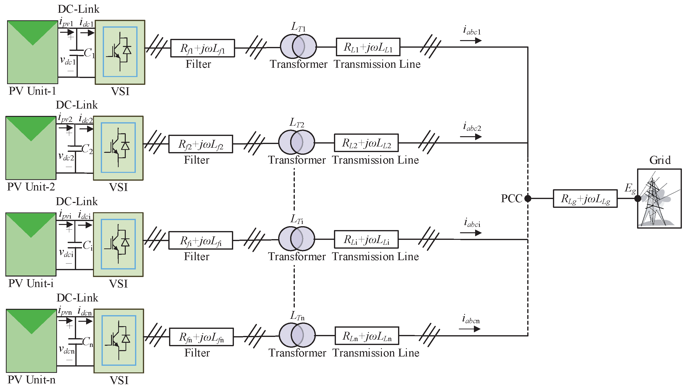
In this paper, it is considered that multiple PV units are connected to the grid through a PCC as shown in Figure 1. In this section, a generalized case is considered where n numbers of PV units are connected together. In Figure 1, each PV unit is first connected to the PCC via the VSI, filter, transformer, and connecting lines. The PCC then connects all PV units to the grid through another connecting line. The detailed dynamical model of grid-connected PV systems with such a configuration is developed in [2] and, for ${\mathrm{i}}^{\mathrm{th}}$ PV unit, it can be summarized through the following equations:

$$\begin{array}{cc}\hfill {\dot{I}}_{d\mathrm{i}}& =-\frac{R_{\mathrm{i}}^{\prime }}{L_{\mathrm{i}}^{\prime }}{I}_{d\mathrm{i}}+\omega I_{q\mathrm{i}}-\frac{E_d}{L_{\mathrm{i}}^{\prime }}+\frac{v_{dc\mathrm{i}}}{L_{\mathrm{i}}^{\prime }}{K}_{d\mathrm{i}}+{\zeta }_{d\mathrm{i}},\hfill \\ \hfill {\dot{I}}_{q\mathrm{i}}& =-\frac{R_{\mathrm{i}}^{\prime }}{L_{\mathrm{i}}^{\prime }}{I}_{q\mathrm{i}}-\omega I_{d\mathrm{i}}-\frac{E_q}{L_{\mathrm{i}}^{\prime }}+\frac{v_{dc\mathrm{i}}}{L_{\mathrm{i}}^{\prime }}{K}_{q\mathrm{i}}+{\zeta }_{q\mathrm{i}},\hfill \\ \hfill {\dot{v}}_{dc\mathrm{i}}& =\frac{1}{C_{\mathrm{i}}}{i}_{pv\mathrm{i}}-\frac{1}{C_{\mathrm{i}}}{I}_{d\mathrm{i}}{K}_{d\mathrm{i}}-\frac{1}{C_{\mathrm{i}}}{I}_{q\mathrm{i}}{K}_{q\mathrm{i}},\hfill \end{array}$$

(1)

where $I_{d\mathrm{i}}$ is the d-axis current of ${\mathrm{i}}^{\mathrm{th}}$ PV unit; $I_{q\mathrm{i}}$ is the q-axis current of ${\mathrm{i}}^{\mathrm{th}}$ PV unit; $E_d$ is the d-axis grid voltage which is actually the d-axis component of the PCC voltage; $E_q$ is the q-axis grid voltage, which is actually the q-axis component of the PCC voltage; $K_{d\mathrm{i}}$ is the d-axis switching control input of the VSI in ${\mathrm{i}}^{\mathrm{th}}$ PV unit which is the d-axis component of the control input; $K_{q\mathrm{i}}$ is the q-axis switching control input of the VSI in ${\mathrm{i}}^{\mathrm{th}}$ PV unit which is the q-axis component of the control input; $R_{\mathrm{i}}^{\prime }=R_{f\mathrm{i}}+R_{L\mathrm{i}}+R_g$ is the total resistance with $R_{f\mathrm{i}}$ as the resistance of the filter in ${\mathrm{i}}^{\mathrm{th}}$ PV unit, $R_{L\mathrm{i}}$ as the resistance of the line in ${\mathrm{i}}^{\mathrm{th}}$ PV unit, and $R_g$ as the resistance of the line connecting the PCC to the grid; $L_{\mathrm{i}}^{\prime }=L_{f\mathrm{i}}+L_{L\mathrm{i}}+L_g$ is the total inductance with $R_{f\mathrm{i}}$ as the inductance of the filter in ${\mathrm{i}}^{\mathrm{th}}$ PV unit, $L_{L\mathrm{i}}$ as the inductance of the line in ${\mathrm{i}}^{\mathrm{th}}$ PV unit, and $L_g$ as the inductance of the line connecting the PCC to the grid; $v_{dc\mathrm{i}}$ is the DC-link voltage of ${\mathrm{i}}^{\mathrm{th}}$ PV unit; ${\zeta }_{d\mathrm{i}}=-\frac{1}{L_{\mathrm{i}}^{\prime }}{\sum }_{\begin{array}{c}\mathrm{k}=1\\ \mathrm{k}\ne \mathrm{i}\end{array}}^{\mathrm{n}}{V}_{gd\mathrm{k}}$ represents d-axis interactions among different PV units; and ${\zeta }_{q\mathrm{i}}=-\frac{1}{L_{\mathrm{i}}^{\prime }}{\sum }_{\begin{array}{c}\mathrm{k}=1\\ \mathrm{k}\ne \mathrm{i}\end{array}}^{\mathrm{n}}{V}_{gq\mathrm{k}}$ represents q-axis interactions among different PV units.

The terms ${\zeta }_{d\mathrm{i}}$ and ${\zeta }_{q\mathrm{i}}$ represent the interactions of other PV units within the system that can be considered as external disturbances or noises. In this paper, the proposed partial feedback linearizing controller is designed based on the dynamical model in Equation (1). In this work, the control objectives are selected as $I_{q\mathrm{i}}$ and $v_{dc\mathrm{i}}$ by considering the maximum power extraction from the PV unit as well as the unity power factor operation and there are two control inputs $K_{d\mathrm{i}}$ and $K_{q\mathrm{i}}$. With these control objectives and inputs, the generalized nonlinear system corresponding to Equation (1) can be written as follows:

$$\begin{array}{cc}\hfill {\dot{x}}_{\mathrm{i}}& =f_{\mathrm{i}}\left(x_{\mathrm{i}}\right)+g_{\mathrm{i}}\left(x_{\mathrm{i}}\right)u_{\mathrm{i}},\hfill \\ \hfill y_{\mathrm{i}}& =h_{\mathrm{i}}\left(x_{\mathrm{i}}\right),\hfill \end{array}$$

(2)

with

$$x_{\mathrm{i}}={\left[\begin{array}{ccc}{I}_{d\mathrm{i}}& I_{q\mathrm{i}}& v_{dc\mathrm{i}}\end{array}\right]}^T,$$

$$f_{\mathrm{i}}\left(x_{\mathrm{i}}\right)=\left[\begin{array}{c}-\frac{R_{\mathrm{i}}^{\prime }}{L_{\mathrm{i}}^{\prime }}{I}_{d\mathrm{i}}+\omega I_{q\mathrm{i}}-\frac{E_d}{L_{\mathrm{i}}^{\prime }}+{\zeta }_{d\mathrm{i}}\\ -\frac{R_{\mathrm{i}}^{\prime }}{L_{\mathrm{i}}^{\prime }}{I}_{q\mathrm{i}}-\omega I_{d\mathrm{i}}-\frac{E_q}{L_{\mathrm{i}}^{\prime }}+{\zeta }_{q\mathrm{i}}\\ \frac{1}{C_{\mathrm{i}}}{i}_{pv\mathrm{i}}\end{array}\right],$$

$$g_{\mathrm{i}}\left(x_{\mathrm{i}}\right)={\left[\begin{array}{cc}\frac{v_{dc\mathrm{i}}}{L_{\mathrm{i}}^{\prime }}& 0\\ 0& \frac{v_{dc\mathrm{i}}}{L_{\mathrm{i}}^{\prime }}\\ -\frac{1}{C_{\mathrm{i}}}{I}_{d\mathrm{i}}& -\frac{1}{C_{\mathrm{i}}}{I}_{q\mathrm{i}}\end{array}\right]}^T,$$

$$u_{\mathrm{i}}={\left[\begin{array}{cc}{K}_{d\mathrm{i}}& K_{q\mathrm{i}}\end{array}\right]}^T,$$

and

$$h_{\mathrm{i}}(x_{\mathrm{i}})={\left[\begin{array}{cc}{I}_{q\mathrm{i}}& v_{dc\mathrm{i}}\end{array}\right]}^T.$$

The design of a partial feedback linearizing controller for ${\mathrm{i}}^{\mathrm{th}}$ PV unit is discussed in the following section.

3. Partial Feedback Linearizing Model Predictive Controller Design for Multiple PV Units Connected to Grids through a PCC

Different steps to design partial feedback linearizing model predictive controllers for ${\mathrm{i}}^{\mathrm{th}}$ PV unit in a grid-connected system with multiple PV units as shown in Figure 1 are discussed in the following:

• Step 1: Calculation of relative degree for $I_{q\mathrm{i}}$ and $v_{dc\mathrm{i}}$

As there are two outputs, the relative degree needs to be calculated for each output. The relative degree ($r_{1\mathrm{i}}$) for the first output function ($I_{q\mathrm{i}}$) will be 1 as the following condition is satisfied:

$$\begin{array}{cc}\hfill L_{g_i}{L}_{f_i}^{1-1}{h}_{1i}\left(x_i\right)& =L_{g_i}{h}_{1i}\left(x_i\right)=\frac{\partial h_{1i}}{\partial x_i}{g}_i=[010]g_i=\frac{v_{dc\mathrm{i}}}{L_{\mathrm{i}}^{\prime }}\ne 0,\hfill \end{array}$$

(3)

where the term $L_{g_i}{h}_{1i}$ defines the Lie derivative of $h_{1i}$ along the vector field $g_i$.

In a similar way, the relative degree ($r_{2i}$) for the second output function ($v_{dc\mathrm{i}}$) will be 1 as the following condition holds:

$$\begin{array}{cc}\hfill L_{g_i}{L}_{f_i}^{1-1}{h}_{2i}\left(x_i\right)& =\frac{v_{dc\mathrm{i}}}{L_{\mathrm{i}}^{\prime }}\ne 0.\hfill \end{array}$$

(4)

Thus, ${\mathrm{i}}^{\mathrm{th}}$ PV unit will have a total relative degree of 2, i.e., $r_{\mathrm{i}}=r_{1\mathrm{i}}+r_{2\mathrm{i}}=2$ though the order of each PV unit is 3, i.e., $n_{\mathrm{i}}=3$. This clearly indicates that the system is partially linearized and the dynamics of the partially linearized system are represented in the following step:

• Step 2: Dynamics of ${\mathrm{i}}^{\mathrm{th}}$ partially linearized PV unit

The dynamic for the nonlinear coordinate transformation corresponding the first output ($I_{q\mathrm{i}}$) can be written as follows:

$$\begin{array}{cc}\hfill {\dot{\tilde{z}}}_{1\mathrm{i}}& =L_{f_{\mathrm{i}}}(I_{q\mathrm{i}})={\tilde{v}}_{1\mathrm{i}},\hfill \end{array}$$

(5)

where

$$\begin{array}{cc}\hfill {\tilde{v}}_{1\mathrm{i}}& =-\frac{R_{\mathrm{i}}^{\prime }}{L_{\mathrm{i}}^{\prime }}{I}_{q\mathrm{i}}-\omega I_{d\mathrm{i}}-\frac{E_q}{L_{\mathrm{i}}^{\prime }}+{\zeta }_{q\mathrm{i}}.\hfill \end{array}$$

(6)

Similarly, the dynamic for the nonlinear coordinate transformation corresponding to the second output ($v_{dc\mathrm{i}}$) can be written as follows:

$$\begin{array}{cc}\hfill {\dot{\tilde{z}}}_{2\mathrm{i}}& =L_{f_{\mathrm{i}}}(v_{dc\mathrm{i}})={\tilde{v}}_{2\mathrm{i}},\hfill \end{array}$$

(7)

where

$$\begin{array}{cc}\hfill {\tilde{v}}_{2\mathrm{i}}& =\frac{1}{C_{\mathrm{i}}}{i}_{pv\mathrm{i}}-\frac{1}{C_{\mathrm{i}}}{I}_{d\mathrm{i}}{K}_{d\mathrm{i}}-\frac{1}{C_{\mathrm{i}}}{I}_{q\mathrm{i}}{K}_{q\mathrm{i}}.\hfill \end{array}$$

(8)

Equations (5) and (7) represent two decoupled linear subsystems for ${\mathrm{i}}^{\mathrm{th}}$ PV unit with $A_{p\mathrm{i}}=\left[0\right]$, $B_{p\mathrm{i}}=\left[1\right]$, and $C_{p\mathrm{i}}=\left[1\right]$ for both subsystems. These equations are actually first-order linear equations, which are obtained from the nonlinear coordinate transformations and independent of operating points. If linear controllers are designed for these linear subsystems using any linear control technique, these will be able to provide stable operation under any operating condition. Thus, linear controllers need to be designed for these two subsystem while the original control inputs $M_{d\mathrm{i}}$ and $M_{q\mathrm{i}}$ can be obtained using Equations (6) and (8). Since the total relative degree is 2 and the order is 3, it is essential to analyze the effects of the remaining dynamic on the stability of the system, which is discussed in the following step.

• Step 3: Dynamical stability analysis of the remaining dynamic

Since the controllers need to be designed in such a way that $\tilde{z}=0$ as $t\to \infty$, the control actions will steer the transformed states, i.e., ${\tilde{z}}_{1\mathrm{i}}$ and ${\tilde{z}}_{2\mathrm{i}}$ towards the desired trajectory. This clearly indicates that ${\tilde{z}}_{1\mathrm{i}}={\tilde{z}}_{2\mathrm{i}}=0$ and thus, ${\dot{\tilde{z}}}_{1\mathrm{i}}={\dot{\tilde{z}}}_{2\mathrm{i}}=0$.

The nonlinear coordinate transformation (${\widehat{\varphi }}_{\mathrm{i}}$) of the remaining dynamic will satisfy $L_{g_i}{\widehat{\varphi }}_{\mathrm{i}}=0$ if it is selected as follows:

$$\begin{array}{cc}\hfill {\widehat{\varphi }}_{\mathrm{i}}& ={\widehat{z}}_{3\mathrm{i}}=\frac{1}{2}{L}_{\mathrm{i}}^{\prime }{I}_{d\mathrm{i}}^2+\frac{1}{2}{L}_{\mathrm{i}}^{\prime }{I}_{q\mathrm{i}}^2+\frac{1}{2}{C}_{\mathrm{i}}{v}_{dc\mathrm{i}}^2.\hfill \end{array}$$

(9)

The remaining dynamic of ${\mathrm{i}}^{\mathrm{th}}$ PV unit can be written as follows:

$$\begin{array}{cc}\hfill {\dot{\widehat{z}}}_{3\mathrm{i}}& =L_{f_{\mathrm{i}}}{\widehat{\varphi }}_{\mathrm{i}}=L_{\mathrm{i}}^{\prime }{I}_{d\mathrm{i}}{f}_{1\mathrm{i}}+L_{\mathrm{i}}^{\prime }{I}_{q\mathrm{i}}{f}_{2\mathrm{i}}+C_{\mathrm{i}}{v}_{dc\mathrm{i}}{f}_{3\mathrm{i}}.\hfill \end{array}$$

(10)

Using $I_{q\mathrm{i}}={\tilde{z}}_{1\mathrm{i}}=0$ and $v_{dc\mathrm{i}}={\tilde{z}}_{2\mathrm{i}}=0$ as well as considering $E_{d\mathrm{i}}=0$, Equation (10) can finally be simplified as follows [28]:

$$\begin{array}{cc}\hfill {\dot{\widehat{z}}}_{3\mathrm{i}}& =-\frac{2R_{\mathrm{i}}^{\prime }}{L_{\mathrm{i}}^{\prime }}{\widehat{z}}_{3\mathrm{i}}+L_{\mathrm{i}}^{\prime }{I}_{q\mathrm{i}}{\zeta }_{q\mathrm{i}}.\hfill \end{array}$$

(11)

The term that includes external disturbance on the right-side of Equation (11) will be vanished individual control actions of other PV units as this is related to the dynamics of q-axis currents of all PV units except ${\mathrm{i}}^{\mathrm{th}}$ PV unit. For this reason, Equation (11) can be simplified as follows:

$$\begin{array}{cc}\hfill {\dot{\widehat{z}}}_{3\mathrm{i}}& =-\frac{2R_{\mathrm{i}}^{\prime }}{L_{\mathrm{i}}^{\prime }}{\widehat{z}}_{3\mathrm{i}}.\hfill \end{array}$$

(12)

Since the values of $R_{\mathrm{i}}$ and $L_{\mathrm{i}}$ are always positive, Equation (12) represents a stable dynamical system. Thus, it can be said that the remaining dynamic of ${\mathrm{i}}^{\mathrm{th}}$ PV unit is stable and the proposed partial feedback linearizing control scheme can employed for the grid-connected system with multiple PV units. At this point, it is essential to design linear controllers for each feedback linearized subsystem of ${\mathrm{i}}^{\mathrm{th}}$ PV unit as discussed in the following step.

• Step 4: Linear model predictive controller design for ${\mathrm{i}}^{\mathrm{th}}$ feedback linearized PV units

For each feedback linearized subsystem of ${\mathrm{i}}^{\mathrm{th}}$ PV unit as represented by Equations (5) and (7), the augmented matrices in the form of the triplet (A, B, C) can be written as follows:

$$A=\left[\begin{array}{cc}0& 0\\ 1& 0\end{array}\right],B=\left[\begin{array}{c}1\\ 0\end{array}\right],\mathrm{and}C={\left[\begin{array}{c}0\\ 1\end{array}\right]}^T.$$

The gains can be calculated by employing continuous-time model predictive control scheme and for each subsystem, the values of these gains will be similar as the order of these subsystems is same. Applying the model predictive control scheme as presented in [32], the linear control input can be written as follows:

$$\begin{array}{cc}\hfill {\dot{\tilde{v}}}_{\mathrm{i}}& =-K_{mpc\mathrm{i}}{\tilde{z}}_{\mathrm{i}}\hfill \end{array}$$

(13)

with ${\tilde{v}}_{\mathrm{i}}={[{\tilde{v}}_{1\mathrm{i}}{\tilde{v}}_{2\mathrm{i}}]}^T$, $K_{mpc\mathrm{i}}={[K_{1mpc\mathrm{i}}{K}_{2mpc\mathrm{i}}]}^T$, and ${\tilde{z}}_{\mathrm{i}}={[{\tilde{z}}_{1\mathrm{i}}{\tilde{z}}_{2\mathrm{i}}]}^T$. Using a receding horizon model predictive control scheme, the value of the gain ($K_{mpc\mathrm{i}}$) for the first-order linear system can be calculated as follows [33]:

$$\begin{array}{cc}\hfill K_{mpc\mathrm{i}}& =L_{\mathrm{i}}{\left(0\right)}^T{\mathsf{\Omega }}_{\mathrm{i}}^{-1}{\mathsf{\Psi }}_{\mathrm{i}},\hfill \end{array}$$

(14)

where $L_{\mathrm{i}}{\left(0\right)}^T={[L_{1\mathrm{i}}{\left(0\right)}^T{L}_{2\mathrm{i}}{\left(0\right)}^T]}^T$, ${\mathsf{\Omega }}_{\mathrm{i}}^{-1}={[{\mathsf{\Omega }}_{1\mathrm{i}}^{-1}{\mathsf{\Omega }}_{2\mathrm{i}}^{-1}]}^T$, and ${\mathsf{\Psi }}_{\mathrm{i}}={[{\mathsf{\Psi }}_{1\mathrm{i}}{\mathsf{\Psi }}_{2\mathrm{i}}]}^T$. Now, it is essential to calculate the values of $L_1\left(0\right)$, ${\mathsf{\Omega }}_1$, and ${\mathsf{\Psi }}_1$ as these values will be used to determine the gains. The values of $L_1\left(0\right)$, ${\mathsf{\Omega }}_1$, and ${\mathsf{\Psi }}_1$ are presented in the following:

$$\begin{array}{c}\hfill L_1\left(0\right)=\left[\begin{array}{cc}1.7321& 0\end{array}\right],\end{array}$$

$$\begin{array}{c}\hfill {\mathsf{\Omega }}_1=\left[\begin{array}{cc}0.201& 0\\ 0& 1\end{array}\right],\mathrm{and}\end{array}$$

$$\begin{array}{c}\hfill {\mathsf{\Psi }}_1=\left[\begin{array}{cc}0.1478& 0.0277\\ 0& 0\end{array}\right].\end{array}$$

With these values of $L_1\left(0\right)$, ${\mathsf{\Omega }}_1$, and ${\mathsf{\Psi }}_1$; the gains ($K_{1mpc\mathrm{i}}$ and $K_{1mpc\mathrm{i}}$) can be calculated as follows:

$$\begin{array}{c}\hfill K_{1mpc\mathrm{i}}=K_{2mpc\mathrm{i}}=\left[\begin{array}{cc}1.2788& 0.2398\end{array}\right].\end{array}$$

(15)

Finally, these values can be used to calculate the linear control inputs ${\tilde{v}}_{1i}$ and ${\tilde{v}}_{2\mathrm{i}}$ for subsystems in ${\mathrm{i}}^{\mathrm{th}}$ PV unit. With these linear control inputs, the design of partial feedback linearizing model predictive control scheme is discussed in the following step:

• Step 5: Design of partial feedback linearizing model predictive controllers for two subsystems in ${\mathrm{i}}^{\mathrm{th}}$ PV unit.

Equation (6) can be used to obtain the control input $K_{q\mathrm{i}}$ while using the value of ${\tilde{v}}_{1\mathrm{i}}$ from the previous step. At this point, it is assumed that the external disturbance (${\zeta }_{q\mathrm{i}}$) will not have any impact on the overall performance of the systems, i.e., ${\zeta }_{q\mathrm{i}}=0$. With this assumption, the control input $K_{q\mathrm{i}}$ can be written as follows:

$$\begin{array}{cc}\hfill K_{q\mathrm{i}}& =\frac{L_{\mathrm{i}}^{\prime }}{v_{dc\mathrm{i}}}\left({\tilde{v}}_{1\mathrm{i}}+\omega I_{d\mathrm{i}}+\frac{R_{\mathrm{i}}^{\prime }}{L_{\mathrm{i}}^{\prime }}{I}_{q\mathrm{i}}+\frac{E_q}{L_{\mathrm{i}}^{\prime }}\right).\hfill \end{array}$$

(16)

Similarly, Equation (8) can be used to obtain the control input $K_{d\mathrm{i}}$ while using the value of ${\tilde{v}}_{1\mathrm{i}}$ from the previous step and $K_{q\mathrm{i}}$ from Equation (16). The control input $K_{d\mathrm{i}}$ can be written as follows:

$$\begin{array}{cc}\hfill K_{d\mathrm{i}}& =-\frac{C_{\mathrm{i}}}{I_{q\mathrm{i}}}\left[{\tilde{v}}_{2\mathrm{i}}+\frac{i_{pv\mathrm{i}}}{C_{\mathrm{i}}}+\frac{L_{\mathrm{i}}^{\prime }{I}_{d\mathrm{i}}}{v_{dc\mathrm{i}}{C}_{\mathrm{i}}}\left({\tilde{v}}_{1\mathrm{i}}+\omega I_{d\mathrm{i}}+\frac{R_{\mathrm{i}}^{\prime }}{L_{\mathrm{i}}^{\prime }}{I}_{q\mathrm{i}}+\frac{E_q}{L_{\mathrm{i}}^{\prime }}\right)\right].\hfill \end{array}$$

(17)

In this paper, the performance of the designed feedback linearizing model predictive controllers is evaluated based on the control inputs represented by Equations (16) and (17). However, it is essential to validate the assumption of ${\zeta }_{q\mathrm{i}}=0$, i.e., the noise or disturbance decoupling capability of the proposed scheme, which is done in the following section.

4. Noise Decoupling Capability of Partial Feedback Linearizing Controllers

If $D_{\mathrm{i}}$ represents the vector related to the external noises and $p_{\mathrm{i}}$ is the noise input, the nonlinear dynamical equation of $i^{th}$ PV unit in a grid-connected PV system as represented by Equation (2) can be rewritten as follows:

$$\begin{array}{cc}\hfill {\dot{x}}_{\mathrm{i}}& =f_{\mathrm{i}}(x_{\mathrm{i}})+g_{\mathrm{i}}(x_{\mathrm{i}})u_{\mathrm{i}}+D_{\mathrm{i}}{p}_{\mathrm{i}},\hfill \\ \hfill y_{\mathrm{i}}& =h_{\mathrm{i}}(x_{\mathrm{i}}).\hfill \end{array}$$

(18)

Since the total relative degree of $i^{th}$ PV unit is ($r_{\mathrm{i}}$), the external noises will be decoupled with the following control input:

$$\begin{array}{cc}\hfill u_{\mathrm{i}}& =a_{\mathrm{i}}(x_{\mathrm{i}})+b_{\mathrm{i}}(x_{\mathrm{i}})v_{\mathrm{i}}\hfill \end{array}$$

(19)

iff the following condition is satisfied:

$$\begin{array}{c}\hfill L_{D_{\mathrm{i}}}{L}_{f_{\mathrm{i}}}^{\mathrm{j}}{h}_{\mathrm{i}}\left(x_{\mathrm{i}}\right)=0\mathrm{for}0\le \mathrm{j}\le r_{\mathrm{i}}-1,\end{array}$$

(20)

where $a_{\mathrm{i}}\left(x_{\mathrm{i}}\right)=L_{f_{\mathrm{i}}}^{r_{\mathrm{i}}}{h}_{\mathrm{i}}(x_{\mathrm{i}})$ and $b_{\mathrm{i}}(x_{\mathrm{i}})=L_{g_{\mathrm{i}}}{L}_{f_{\mathrm{i}}}^{r_{\mathrm{i}}-1}{h}_{\mathrm{i}}(x_{\mathrm{i}})$.

In order to justify the noise decoupling capability of the control input (19), it is essential to substitute this control input into Equation (18) and, by doing this, it can be written as follows:

$$\begin{array}{cc}\hfill {\dot{x}}_{\mathrm{i}}& =f_{\mathrm{i}}\left(x_{\mathrm{i}}\right)+g_{\mathrm{i}}\left(x_{\mathrm{i}}\right)a_{\mathrm{i}}\left(x_{\mathrm{i}}\right)+g_{\mathrm{i}}\left(x_{\mathrm{i}}\right)b_{\mathrm{i}}\left(x_{\mathrm{i}}\right)v_{\mathrm{i}}+D_{\mathrm{i}}{p}_{\mathrm{i}},\hfill \\ \hfill y_{\mathrm{i}}& =h_{\mathrm{i}}\left(x_{\mathrm{i}}\right).\hfill \end{array}$$

(21)

From Equation (21), it can be seen that the output variable $y_{\mathrm{i}}$ does not depend on the external disturbances even for the case when $v_{\mathrm{i}}=0$. By considering this situation, i.e., $v_{\mathrm{i}}=0$, Equation (21) can be simplified as follows:

$$\begin{array}{cc}\hfill {\dot{x}}_{\mathrm{i}}& ={\overline{f}}_{\mathrm{i}}\left(x_{\mathrm{i}}\right)+{\overline{g}}_{\mathrm{i}}\left(x_{\mathrm{i}}\right){\overline{u}}_{\mathrm{i}},\hfill \\ \hfill y_{\mathrm{i}}& =h_{\mathrm{i}}\left(x_{\mathrm{i}}\right),\hfill \end{array}$$

(22)

where ${\overline{f}}_{\mathrm{i}}\left(x_{\mathrm{i}}\right)=f_{\mathrm{i}}\left(x_{\mathrm{i}}\right)+g_{\mathrm{i}}\left(x_{\mathrm{i}}\right)a_{\mathrm{i}}\left(x_{\mathrm{i}}\right)$, ${\overline{g}}_{\mathrm{i}}\left(x_{\mathrm{i}}\right)=D_{\mathrm{i}}\left(x_{\mathrm{i}}\right)$, and ${\overline{u}}_{\mathrm{i}}=p_{\mathrm{i}}$.

Equation (22) has the similar form of a nonlinear system and the first nonlinear coordinate transformation for this system can be written as follows:

$$\begin{array}{cc}\hfill {\dot{y}}_{\mathrm{i}}& =\frac{\partial h_{\mathrm{i}}\left(x_{\mathrm{i}}\right)}{\partial x_{\mathrm{i}}}{\dot{x}}_{\mathrm{i}}=\frac{\partial h_{\mathrm{i}}\left(x_{\mathrm{i}}\right)}{\partial x_{\mathrm{i}}}\left[{\overline{f}}_{\mathrm{i}}\left(x_{\mathrm{i}}\right)+{\overline{g}}_{\mathrm{i}}\left(x_{\mathrm{i}}\right){\overline{u}}_{\mathrm{i}}\right]=L_{{\overline{f}}_{\mathrm{i}}}{h}_{\mathrm{i}}\left(x_{\mathrm{i}}\right)+L_{{\overline{g}}_{\mathrm{i}}}{h}_{\mathrm{i}}\left(x_{\mathrm{i}}\right){\overline{u}}_{\mathrm{i}}.\hfill \end{array}$$

(23)

Equation (23) clearly indicates that the output will be decoupled from the noise (${\overline{u}}_{\mathrm{i}}=p_{\mathrm{i}}$) if $L_{{\overline{g}}_{\mathrm{i}}}{h}_{\mathrm{i}}\left(x_{\mathrm{i}}\right)=0$.

Similarly, the second nonlinear coordinate transformation can be written as follows:

$$\begin{array}{cc}\hfill {\ddot{y}}_{\mathrm{i}}& =L_{{\overline{f}}_{\mathrm{i}}}^2{h}_{\mathrm{i}}\left(x_{\mathrm{i}}\right)+L_{{\overline{g}}_{\mathrm{i}}}{L}_{{\overline{f}}_{\mathrm{i}}}{h}_{\mathrm{i}}\left(x_{\mathrm{i}}\right){\overline{u}}_{\mathrm{i}}\hfill \end{array}$$

(24)

for which the output will be independent of noises if $L_{{\overline{g}}_{\mathrm{i}}}{L}_{{\overline{f}}_{\mathrm{i}}}{h}_{\mathrm{i}}\left(x_{\mathrm{i}}\right)=0$.

Finally, $r_{\mathrm{i}}^{th}$ nonlinear coordinate transformation can be written as follows:

$$\begin{array}{cc}\hfill {\dot{y}}_{\mathrm{i}}^{r_{\mathrm{i}}}& =L_{{\overline{f}}_{\mathrm{i}}}^{r_{\mathrm{i}}}{h}_{\mathrm{i}}\left(x_{\mathrm{i}}\right)+L_{{\overline{g}}_{\mathrm{i}}}{L}_{{\overline{f}}_{\mathrm{i}}}^{r_{\mathrm{i}}-1}{h}_{\mathrm{i}}\left(x_{\mathrm{i}}\right){\overline{u}}_{\mathrm{i}},\hfill \end{array}$$

(25)

where the noise decoupled output can be obtained if the following condition holds:

$$\begin{array}{c}\hfill L_{{\overline{g}}_{\mathrm{i}}}{L}_{{\overline{f}}_{\mathrm{i}}}^{r_{\mathrm{i}}-1}{h}_{\mathrm{i}}\left(x_{\mathrm{i}}\right)=0.\end{array}$$

(26)

Finally, Equation (26) can be represented in the following generalized form:

$$\begin{array}{c}\hfill L_{{\overline{g}}_{\mathrm{i}}}{L}_{{\overline{f}}_{\mathrm{i}}}^{\mathrm{j}}{h}_{\mathrm{i}}\left(x_{\mathrm{i}}\right)=0\mathrm{for}0\le \mathrm{j}\le r_{\mathrm{i}}-1,\end{array}$$

(27)

which can actually be rewritten as

$$\begin{array}{c}\hfill L_{D_{\mathrm{i}}}{L}_{(f_{\mathrm{i}}+g_{\mathrm{i}}{a}_{\mathrm{i}})}^{\mathrm{j}}{h}_{\mathrm{i}}\left(x_{\mathrm{i}}\right)=0\mathrm{for}0\le \mathrm{j}\le r_{\mathrm{i}}-1.\end{array}$$

(28)

Using the definition of relative degree, it can be written as follows:

$$\begin{array}{c}\hfill L_{(f_{\mathrm{i}}+g_{\mathrm{i}}{a}_{\mathrm{i}})}^{\mathrm{j}}{h}_{\mathrm{i}}\left(x_{\mathrm{i}}\right)=L_{f_{\mathrm{i}}}^{\mathrm{j}}{h}_{\mathrm{i}}\left(x_{\mathrm{i}}\right)\mathrm{for}0\le \mathrm{j}\le r_{\mathrm{i}}-1.\end{array}$$

(29)

Finally, using Equation (29), Equation (28) can be simplified as follows:

$$\begin{array}{c}\hfill L_{D_{\mathrm{i}}}{L}_{f_{\mathrm{i}}}^{\mathrm{j}}{h}_{\mathrm{i}}\left(x_{\mathrm{i}}\right)=0\mathrm{for}0\le \mathrm{j}\le r_{\mathrm{i}}-1.\end{array}$$

(30)

Therefore, the assumption made in Equation (20) stands in relation to the noise decoupling capability of partial feedback linearizing controllers. This also clearly indicates the applicability of the designed controller in the previous section. The performance of the designed partial feedback linearizing controller is evaluated in the following section.

5. Controller Performance Evaluation

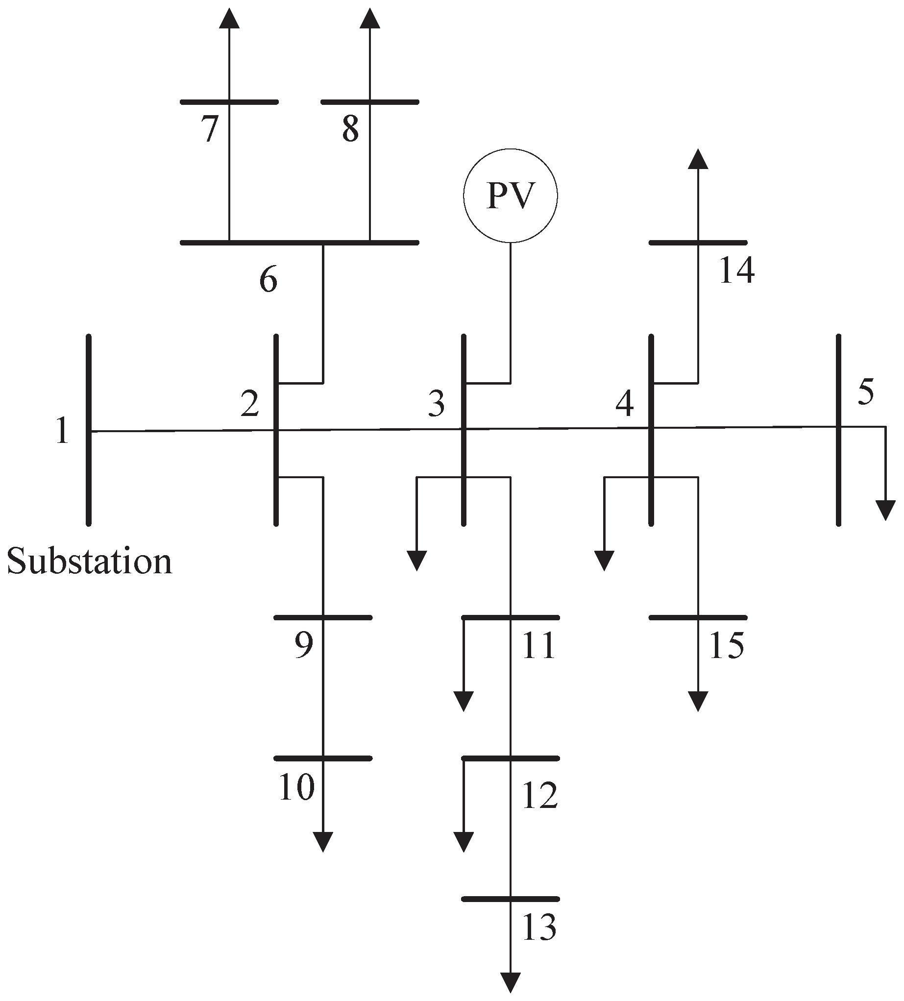
The performance of designed controllers is evaluated on an IEEE 15-bus radial distribution network as shown in Figure 2. The detailed line and load parameters of this 15-bus network can be found in [34]. In this paper, the test system is modified by connected three solar PV units (PV-1, PV-2, and PV-3) at bus-3. The capacities of PV-1, PV-2, and PV-3 are 6.1 kW, 9.5 kW, and 3.29 kW, respectively, while the load demand in the system is 18.903 MW. These PV units are connected at bus-3 with the configuration as shown in Figure 1. The detailed parameters for this configurations with these three PV units can be found in [2]. The PV units in this system supplies only a small portion of the network and the remaining power is supplied from the slack bus. The inclusions of these small-scale PV units might not have significant effects on the overall performance of the system. However, there will be significant deteriorations of the power quality in the currents injected into the bus at which all these PV units are connected. In this paper, the designed controller is employed with each PV unit and the performances of these controllers are evaluated through simulation studies by considering the following three case studies:

• Controller performance evaluation under standard atmospheric conditions,
• Controller performance evaluation under changing atmospheric conditions, and
• Controller performance evaluation under a single-phase to ground fault.

The simulation studies are carried out in MATLAB/SIMULINK and the detailed discussions are provided in the following. The performances are also compared with an existing PI controller.

● Case 1: Controller performance evaluation under standard atmospheric conditions

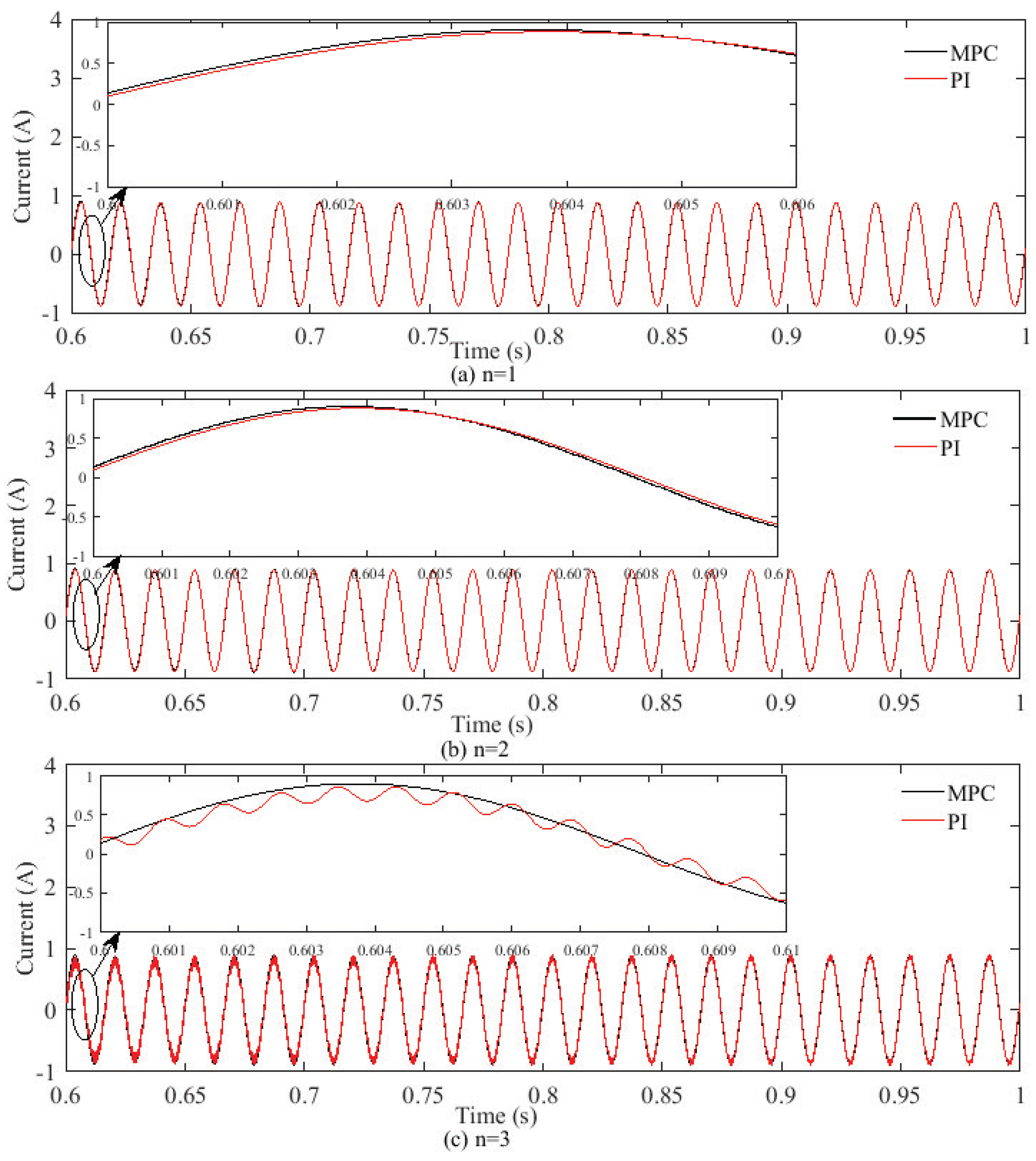
When the standard atmospheric conditions are considered, the solar irradiation (which is related to the solar insolation) is generally considered as 1000 Wm${}^{-2}$ and the environmental temperature as 298 K. In this work, the plane of array model is used during the simulation to calculate the available energy from the sun for a particular time on a surface with fixed-tilt and azimuth. At this condition, the module temperature is considered as 306 K. Under this condition, the output current of PV-2 is continuously monitored with increases in the number of PV units. Figure 3a shows the current of PV-2 when no other PV units are integrated with the grid while Figure 3b,c show the current responses with $n=2$ and $n=3$, respectively, where the values of n indicate the total number of PV units. From Figure 3, it can be seen that the current responses are distorted with the increases in PV units. However, these distortions are more when the PI controllers are used while comparing with these responses with designed partial feedback linearizing model predictive controllers (shortly, MPC in all figures). This clearly indicates that the power quality of the system degrades due to the inclusions of more PV units into existing power grids.

Under this operating condition, the output current responses of other PV units, i.e., PV-1 and PV-3 are also monitored to investigate the dynamic interactions among multiple PV units. However, these responses are not presented here; instead, the power quality is investigated. The power quality issues can be discussed in terms of total harmonic distortions (THDs). The THD is generally defined as the ratio of the root mean square (RMS) amplitude for a waveform having a number of higher harmonic frequencies other than the fundamental frequency and the RMS of the same waveform at the fundamental frequency [35]. Practically, the acceptable limits of THDs due to the integration of distributed generation is 5%. The values of THDs under this standard atmospheric condition are shown in

Table 1. The values of THDs with the PI controller for the output currents of PV-1, PV-2, and PV-3 along with the current injected into the grid.

Controller	Current	Standard Condition (THD in %)			Environmental Change (THD in %)
		n = 1	n = 2	n = 3	n = 1	n = 2	n = 3
PI	PV-1	-	-	8.27	-	-	9.03
	PV-2	0.14	0.84	2.81	0.23	2.07	2.98
	PV-3	-	1.77	3.42	-	2.93	3.04

and

Table 2. The values of THDs with the designed controller for the output currents of PV-1, PV-2, and PV-3.

Controller	Current	Standard Condition (THD in %)			Environmental Change (THD in %)
		n = 1	n = 2	n = 3	n = 1	n = 2	n = 3
MPC	PV-1	-	-	1.51	-	-	2.87
	PV-2	0.14	0.45	0.93	0.27	0.88	1.27
	PV-3	-	0.89	1.03	-	1.04	1.14
	Grid	0.14	0.23	0.55	0.14	0.77	0.90

for PI and designed controllers, respectively. From Table 1, it can be seen that the value of the THD is 8.27%, i.e., more than 5% for the output current response of PV-1 when all three PV units are connected together and PI controllers are used with these PV units. On the other hand, Table 2 clearly shows that the values of all THDs under standard atmospheric conditions when the designed controllers are used for all three PV units. Therefore, it can be summarized that existing PI controllers are unable to maintain the desired power quality due to the increases in the PV integration. It is also worth noting that the fluctuations in power, voltage at the PCC, and frequency are not significant under the standard atmospheric conditions when both the designed and PI controllers are used. However, these fluctuations are visible when under changes in atmospheric conditions as well as during the fault conditions, which will be discussed in the following two case studies.

● Case 2: Controller performance evaluation under changing atmospheric conditions

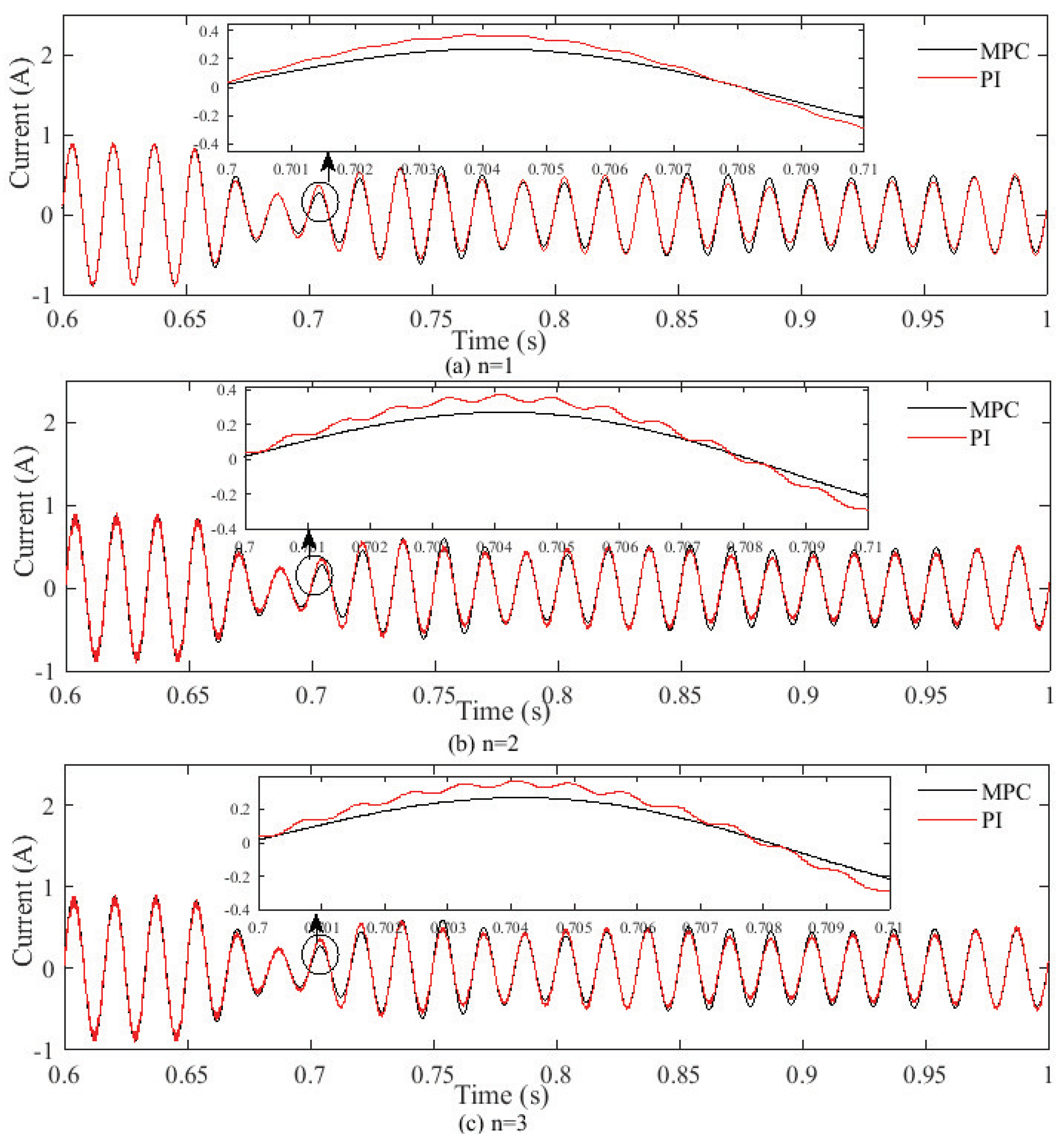
The solar irradiations and environmental temperatures change continuously. In this case study, the changes in solar irradiations are considered as 40% from the nominal value, i.e., the value in the standard atmospheric conditions while all other parameters remain unchanged. In this case study, it is considered that such changes occur at t = 0.65 s. In this situation, the output current responses of PV-2 are again monitored to investigate the performances of both PI and designed model predictive controllers with the increases in the number of PV units within the system. Figure 4 shows these current responses when $n=1$, $n=2$, and $n=3$. The current responses in Figure 4 clearly show that the designed controllers modulate the switching control actions in such a way that there are less distortions as compared to the PI controllers. The DC-link voltage and the output power responses of all PV units are also monitored during the simulations and in all cases, and it is found that the designed controllers perform in a much better way as compared to the existing PI controller.

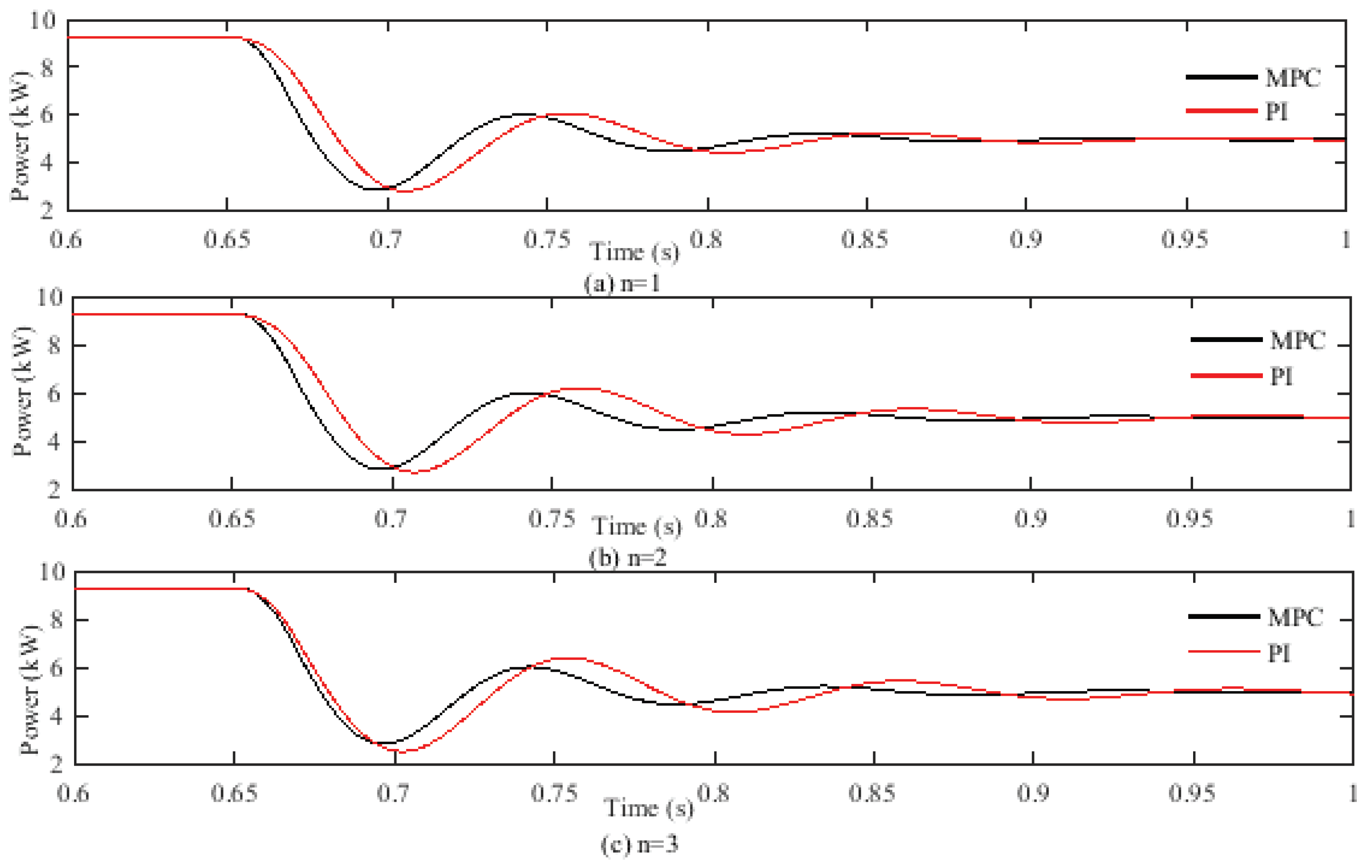
Under this changing atmospheric condition, the output power responses of PV-2 are observed with the increases in PV units. This means that the output power of PV-2 is first observed with $n=1$, i.e., only with PV-2 and then PV-1 and PV-2 are gradually put in service. All these power responses are shown in Figure 5 from where it can be seen that there are more fluctuations with the increases in the number of PV units. 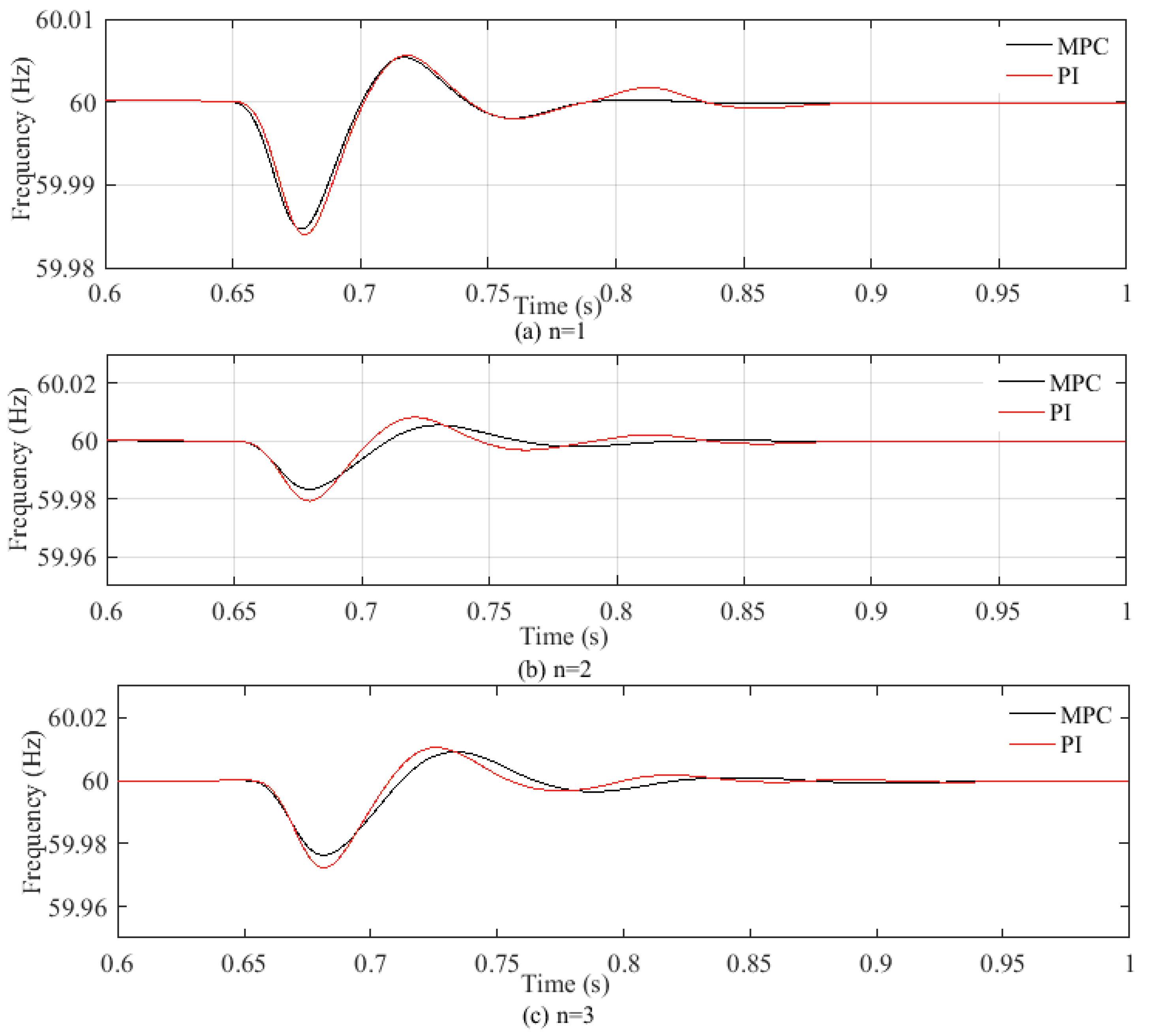However, the designed partial feedback linearizing model predictive controllers tackle these challenges in oscillations in a better way as compared to the PI controller, which can also be seen from Figure 5. At the same time, the voltage at the PCC is also monitored and this voltage is not affected much as the PCC is considered as the reference bus. However, there are variations in the grid frequency due to the variations in the active power, which can be seen from Figure 6. The frequency responses in Figure 5 exhibit similar fluctuation patterns to that of the active power responses where the designed controller acts in a much better way as compared to the PI controller. Therefore, it is clear that the designed partial feedback linearizing controller outperforms the PI controller even under changing atmospheric conditions.

The output current responses of PV-1 and PV-3 are also monitored under changing atmospheric conditions and presented in Table 1 and Table 2 for PI and designed controllers, respectively. Table 1 clearly demonstrates that the values of THDs have further increased due to changes in atmospheric conditions as compared to standard atmospheric condition. The value of the THD for the output current of PV-1 with all PV units (i.e., $n=3$) is now increased to 9.03% when the PI controllers are used. However, the designed controllers still maintain the values of THDs well below the acceptable limit, which can easily be seen from Table 2.

● Case 3: Controller performance evaluation under a single-phase to ground fault

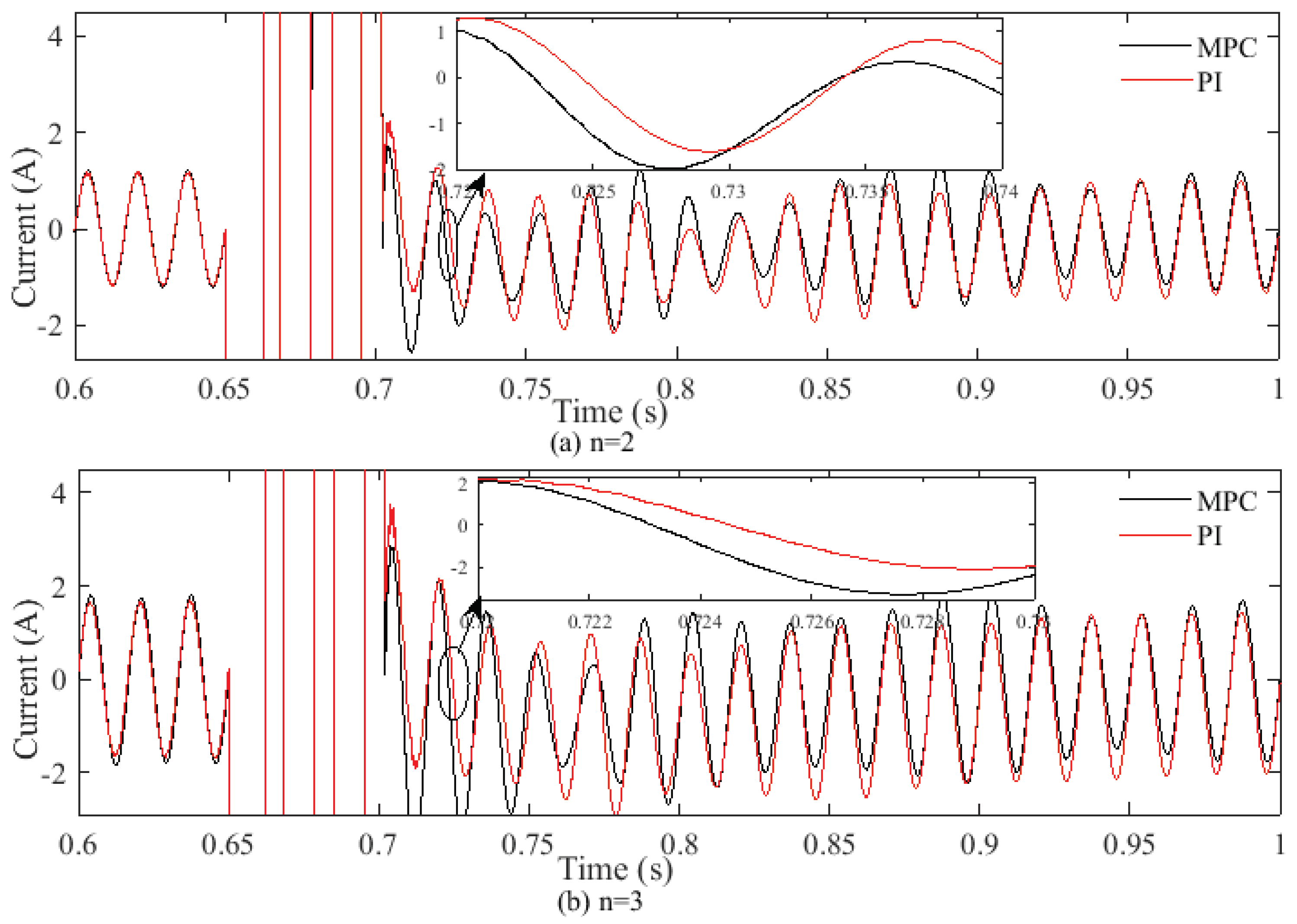
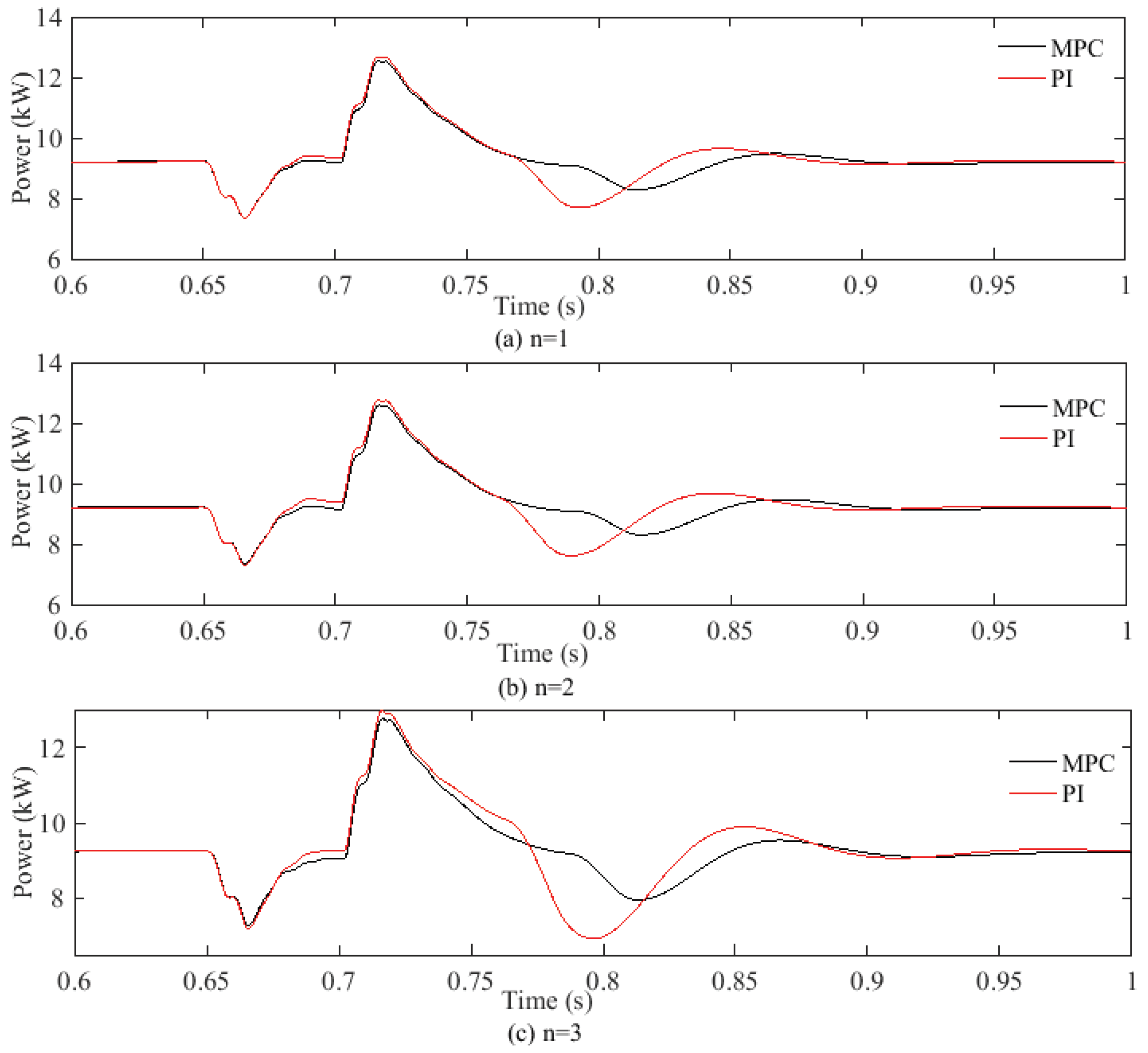
In this case study, a single-phase to ground fault is applied at bus-3 at t = 0.65 s and cleared at 0.70 s under standard atmospheric conditions. In this situation, the grid currents for $n=2$ and $n=3$ are represented in Figure 7a,b, respectively, when both PI and the designed partial feedback linearizing model predictive controllers are used. It is clear that the current increases than the standard condition at the time of contingency. After clearance of the fault, the PI controller takes a longer time to stabilize the output current than the designed controller. 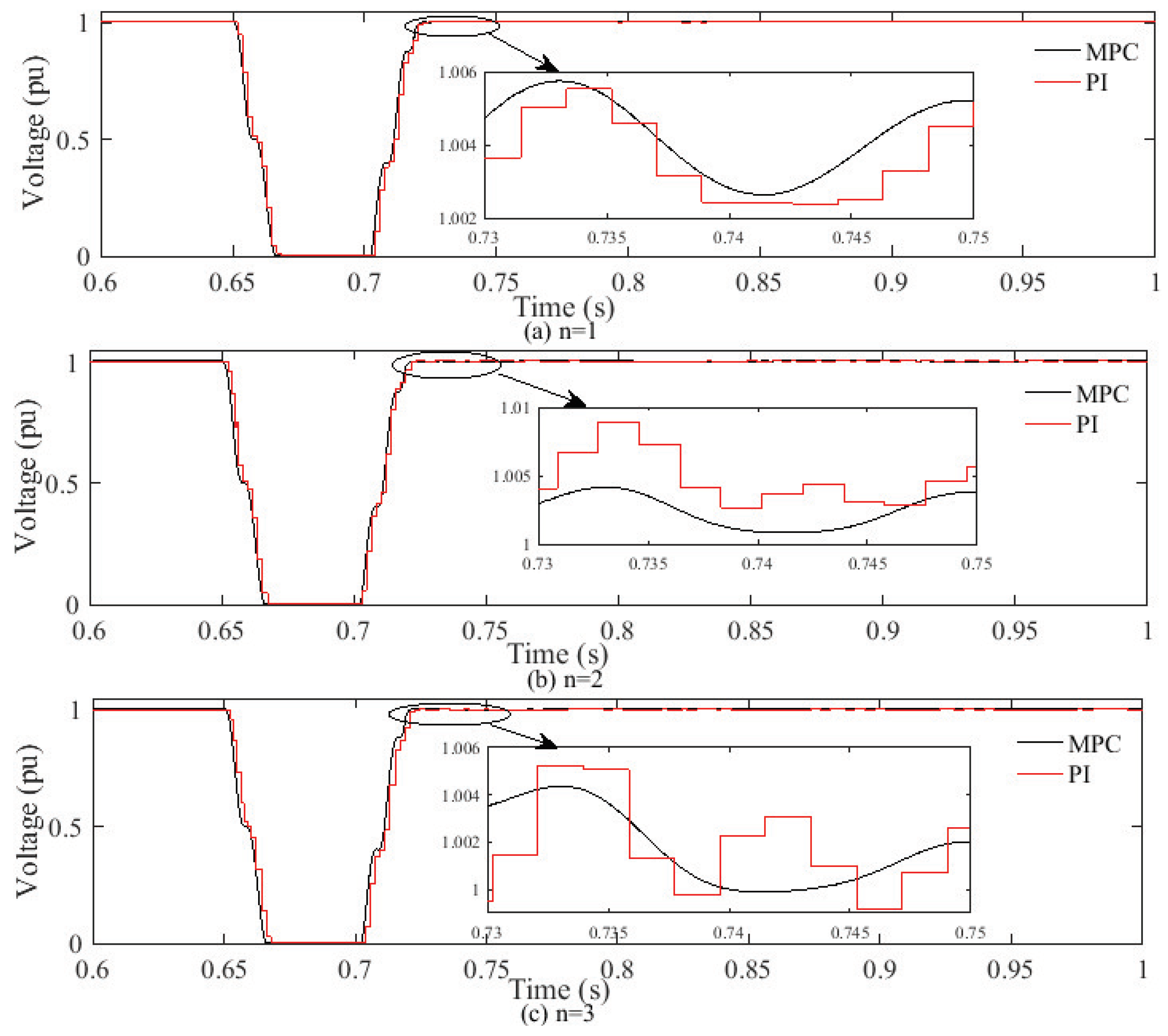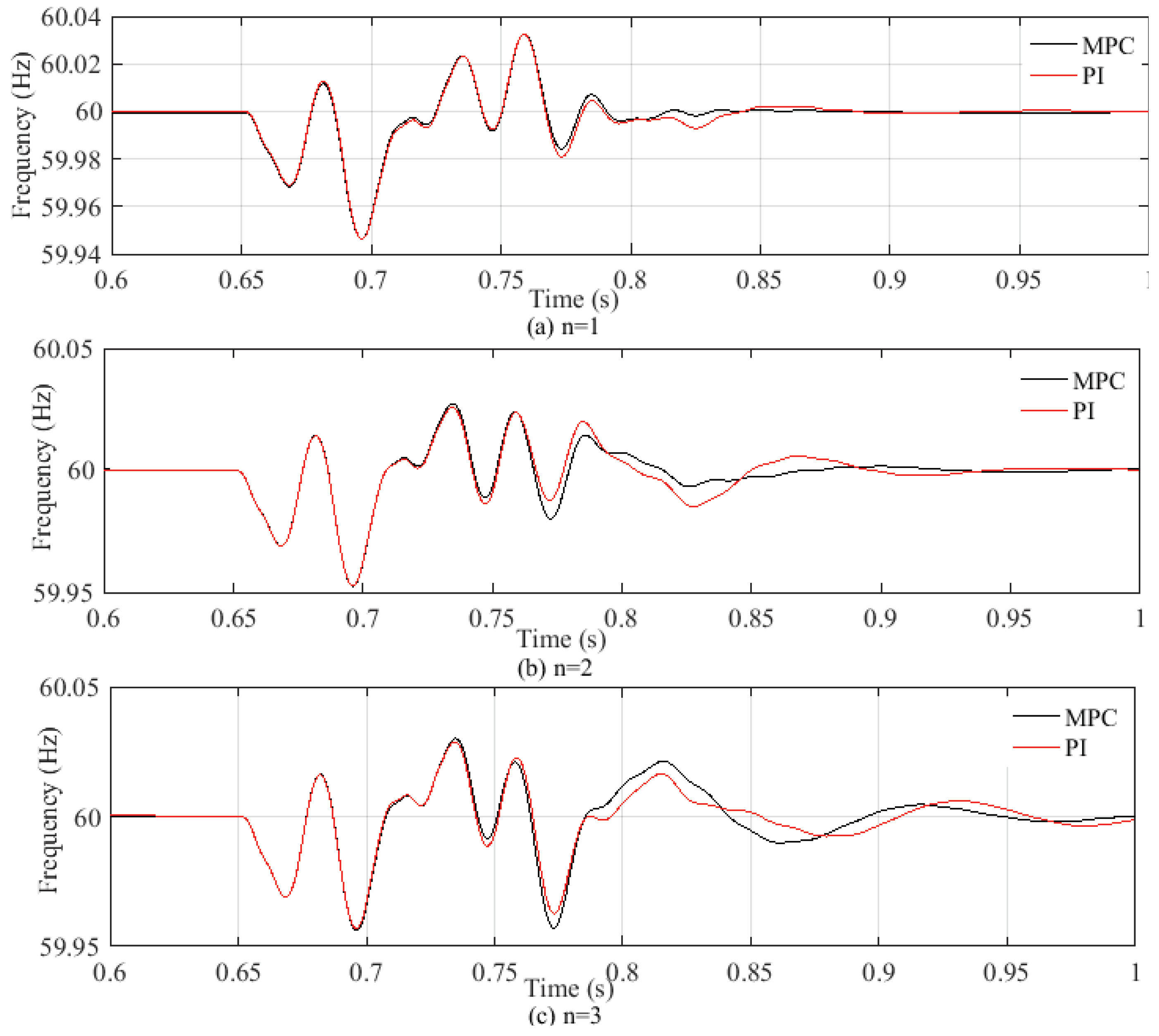Under this condition, the output power of PV-2 is shown in Figure 8 from where it can be seen that the transients are more severe with the increases in the number of PV units. During the faulted period, the voltage at the PCC will be zero and, after the clearance of the fault, the fluctuations in this voltage will be more with the increases in the PV unit, which can be seen from Figure 9 and the frequency responses will also experience similar fluctuations as shown in Figure 10. From these figures, it can be seen that there are less fluctuations when the designed partial feedback linearizing controllers are used with all PV units. Hence, the designed controllers exhibit faster responses and better noise or disturbance decoupling capabilities as compared to PI controllers. Furthermore, these results clearly indicate the fault-ride through capability of the PV system with the designed feedback linearizing model predictive controller.

6. Conclusions

Partial feedback linearizing model predictive controllers are designed for grid-connected systems with multiple PV units where these PV units are connected through the point of common coupling. The designed control scheme simplifies the dynamical models of multiple PV units and eliminates the dynamic interactions among different PV units. Since the designed control scheme reduces the order of the partially linearized system, it becomes faster, which is also made evident from the simulation results. Moreover, the designed controller cancels nonlinearities using nonlinear terms and thus the linearized system is independent of operating points. Simulation results under different operating conditions clearly depict the performance of the controller in terms of maintaining the desired current injection into the grid with the improved power quality. Simulation results under both standard and changing atmospheric conditions demonstrate that existing PI controllers are unable to maintain the acceptable power quality which are not the cases for designed controllers. Future works will deal with the design of robust controllers for based similar models of grid-connected PV systems.