Ice-Crystal Nucleation in Water: Thermodynamic Driving Force and Surface Tension. Part I: Theoretical Foundation


1
Leibniz Institute for Tropospheric Research (TROPOS), Permoserstraße 15, D-04318 Leipzig, Germany
2
Institute of Physics, University of Rostock, Albert-Einstein-Straße 23-25, D-18059 Rostock, Germany
3
Leibniz Institute for Baltic Research (IOW), Seestraße 15, D-18119 Rostock-Warnemünde, Germany
*
Author to whom correspondence should be addressed.
Entropy 2020, 22(1), 50; https://doi.org/10.3390/e22010050
Submission received: 15 September 2019
/
Revised: 17 December 2019
/
Accepted: 19 December 2019
/
Published: 30 December 2019
(This article belongs to the Special Issue Crystallization Thermodynamics)
Abstract
:A recently developed thermodynamic theory for the determination of the driving force of crystallization and the crystal–melt surface tension is applied to the ice-water system employing the new Thermodynamic Equation of Seawater TEOS-10. The deviations of approximative formulations of the driving force and the surface tension from the exact reference properties are quantified, showing that the proposed simplifications are applicable for low to moderate undercooling and pressure differences to the respective equilibrium state of water. The TEOS-10-based predictions of the ice crystallization rate revealed pressure-induced deceleration of ice nucleation with an increasing pressure, and acceleration of ice nucleation by pressure decrease. This result is in, at least, qualitative agreement with laboratory experiments and computer simulations. Both the temperature and pressure dependencies of the ice-water surface tension were found to be in line with the le Chatelier–Braun principle, in that the surface tension decreases upon increasing degree of metastability of water (by decreasing temperature and pressure), which favors nucleation to move the system back to a stable state. The reason for this behavior is discussed. Finally, the Kauzmann temperature of the ice-water system was found to amount , which is far below the temperature of homogeneous freezing. The Kauzmann pressure was found to amount to , suggesting favor of homogeneous freezing on exerting a negative pressure on the liquid. In terms of thermodynamic properties entering the theory, the reason for the negative Kauzmann pressure is the higher mass density of water in comparison to ice at the melting point.
1. Introduction
1.1. Motivation
The outstanding importance of homogeneous freezing for a variety of natural and technical processes such as the microphysical evolution of atmospheric clouds (e.g., Meyers et al. [1], Khvorostyanov and Sassen [2], Lohmann and Kärcher [3], Lohmann et al. [4], Pruppacher and Klett [5], Heymsfield et al. [6], Jensen and Ackerman [7], Barahona and Nenes [8], Jensen et al. [9], Zasetsky et al. [10], Khvorostyanov and Curry [11], Khvorostyanov and Curry [12], Hellmuth et al. [13], Khvorostyanov and Curry [14], Lohmann et al. [15]), the cryopreservation of organelles, cells, tissues, extracellular matrices, organs, and foods (e.g., Pegg [16], Espinosa et al. [17], Espinosa et al. [18], see also https://en.wikipedia.org/wiki/Cryopreservation, visited on December 29, 2019), and water vitrification (e.g., Debenedetti and Stanley [19], Bhat et al. [20], Zobrist et al. [21]) stimulated a highly visible number of investigations on the thermophysical behavior of undercooled and deeply undercooled water
- within the framework of laboratory studies and evaluation of experimental data (e.g., McDonald [22], Butorin and Skripov [23], Hagen et al. [24], Hare and Sorensen [25], Henderson and Speedy [26], Speedy [27], Bartell and Huang [28], Gránásy [29], Huang and Bartell [30], Jeffery and Austin [31], Benz et al. [32], Holten et al. [33], Stöckel et al. [34], Souda [35], Tabazadeh et al. [36], Vortisch et al. [37], Malila and Laaksonen [38], Atkinson et al. [39]),
- by computer simulations (e.g., Gránásy [29,40], Matsumoto et al. [41], Oxtoby [42], Nada et al. [43], Laird and Davidchack [44], Vega and Abascal [45], Bai and Li [46], Bartell and Wu [47], Hernández de la Peña and Kusalik [48], Vega et al. [49], Vrbka and Jungwirth [50], Espinosa et al. [17,18], Moore and Molinero [51], Tanaka and Kimura [52]),
Comprehensive overviews on the fundamental thermodynamic and molecular properties of water and the transition from clusters to liquid are given, e.g., by Ludwig [56], on undercooled and glassy water by Debenedetti [55], and on the notions, methods, and challenges to determine the crystal–melt interfacial free energy by Gránásy [29] and Laird and Davidchack [44]. Basic studies on the thermodynamic behavior of metastable liquids were performed, e.g., by Skripov [57], Skripov and Baidakov [58], Skripov and Koverda [59], Debenedetti et al. [60], Baidakov [61], Baidakov [62], Baidakov [63,64], Baidakov and Protsenko [65,66], Skripov and Faizullin [67], Baidakov et al. [68], Bartell and Wu [69]. In the last decade highly accurate equations of state (EoS) for water and ice became available, which are based on data from the experimentally accessible parts of the phase diagram of water: (i) for stable water (Wagner and Pruß [70], Wagner et al. [71], Guder [72]); (ii) for seawater (Feistel and Hagen [73], Feistel [74,75], Feistel et al. [76]) (iii) for hexagonal ice (Feistel and Hagen [77,78], Feistel and Wagner [79,80,81,82], IAPWS R10-06 [83]), (iii) for undercooled water (Holten et al. [84,85,86]). The application of these EoS’ is supported by the availability of international guidelines and standards for execution (Feistel et al. [87], Wright et al. [88], Feistel [89,90], IAPWS R6-95 [91], IAPWS R10-06 [83], IAPWS [92], IAPWS R13-08 [93], IAPWS [94,95], IAPWS G12-15 [96], IOC, SCOR, and IAPSO [97]). The aforementioned list of works contributing to water-to-ice crystallization, however, must inevitably remain incomplete and can be further extended.
The classical theory of nucleation (CNT) and growth processes is till now the major tool in the interpretation of experimental data on crystal nucleation and growth (e.g., Skripov [57], Skripov and Koverda [59], Skripov and Faizullin [67], Gutzow and Schmelzer [98], Gutzow and Schmelzer [99], Debenedetti [100], Kelton and Greer [101], Herlach et al. [102]). In its physical ingredients it is based on the thermodynamic theory of heterogeneous systems as developed by Josiah W. Gibbs (Gibbs [103,104]). Following Gibbs’ method in the specification of the properties of the critical clusters, it turns out that they correspond widely to the properties of the newly evolving macroscopic phases. This consequence of Gibbs’ theory gives the foundation of one of the main approximations of CNT in application to crystal nucleation, namely the identification of the bulk properties of the critical crystallites with the properties of the evolving macroscopic crystalline phase (Schmelzer and Abyzov [105]).
In line with such approximation, the surface tension in between melt and critical crystal can be identified with the respective value for a planar equilibrium coexistence of the respective liquid and crystalline phases. The latter assumption is denoted commonly as capillarity approximation. In the framework of CNT, frequently a curvature dependence of the surface tension is introduced in order to reconcile theory with experiment while the bulk properties of the critical clusters are assumed to be more or less defined as described above. Moreover, the introduction of a curvature dependence of the surface tension is the major tool to arrive at a correct description of nucleation rates measured experimentally. Alternatively, the theoretical expressions for the kinetic pre-factor in the expression for the steady-state nucleation rate can be modified. However, this approach results as a rule only in minor changes of the theoretical predictions (Gutzow and Schmelzer [98], Gutzow and Schmelzer [99], Skripov and Koverda [59]).
Alternative approaches have been advanced in recent decades based on generalizations of the classical Gibbs’ approach going beyond these simplest approximations (Gutzow and Schmelzer [99], Schmelzer et al. [106], Schmelzer and Abyzov [107]). These methods allow one to describe and in this way also to account for variations of the bulk properties of critical clusters in dependence on the degree of deviation from equilibrium. They are, however, much more complex and not as easily applicable as classical theory. Consequently, at least as a first estimate, CNT based on Gibbs’ classical method of description will also be retained in future to serve as a valuable tool in treating experimental data.
1.2. Rationale of the Present Study
Based on such considerations, in recent papers by Schmelzer and Abyzov [105,108] and Schmelzer et al. [109,110] two of the basic ingredients of CNT were revisited: the methods of specification of the thermodynamic driving force of nucleation and the dependence of the surface tension on the degree of deviation from equilibrium (i.e., the degree of metastability) or, equivalently, on the size of the critical clusters (Schmelzer et al. [111,112]). This analysis was performed for crystal nucleation caused by both variations of temperature and pressure. In particular, it was shown there that for both cases, the Tolman equation can be employed as an appropriate approximation for the description of the curvature dependence of the surface tension and not only for variations of external pressure at isothermal conditions as studied by Tolman [113]. Moreover, also going beyond Tolman’s analysis it is shown that Tolman’s approach can be employed also for multi-component systems provided the composition of the crystal phase (as employed as the basic assumption in CNT) and the composition of the liquid (as it is most frequently studied in crystallization) are considered as or kept constant. Consequences from the basic equations derived were discussed in the cited papers mainly for the most frequently occurring situation that the mass-specific volume of the crystal phase is smaller as compared to the respective value of the liquid phase.
Here, we will discuss the following aspects of ice nucleation in water as a very important example in many respects, wherein the opposite condition is fulfilled, i.e., where the mass-specific volume of the crystal phase is larger as compared to the respective value for the liquid phase:
- (i)
- As the first topic of the analysis, we will explore which qualitative differences arise in the water–ice system in comparison to other systems discussed earlier. Since we restrict the analysis here to a one-component case, it is also reasonable to expect that the basic assumptions of CNT may be fulfilled in a good approximation. At least, such conclusion was drawn quite recently based on molecular dynamics studies of melt crystallization for Lennard–Jones systems (Baidakov [64]). Possible generalizations of the theory in terms of the generalized Gibbs’ approach accounting for variations of density of the critical crystallites (as performed by some of us for the description of condensation and boiling (Schmelzer and Schmelzer Jr. [114,115], Schmelzer and Baidakov [116]), or segregation in solutions (Schmelzer et al. [117], Abyzov and Schmelzer [118], Schmelzer and Abyzov [119])) will not be discussed here. Having in mind the aforementioned importance of ice–crystal nucleation in a variety of processes in nature, we will further analyze in detail the degree of quantitative accuracy in the application of the general relations, derived in the mentioned papers, to this particular realization of crystal nucleation. This concerns the expressions for the temperature and pressure dependencies of the thermodynamic driving force of crystallization and the ice–water surface tension.
- (ii)
- A second aspect of the analysis is the application of the advanced Thermodynamic Equation of Seawater TEOS-10 for the calculation of the thermodynamic properties, which determine the temperature and pressure dependencies of the thermodynamic driving force of crystallization and the ice–water surface tension.
- (iii)
- Finally, the third question of interest is related to a problem already studied by Kauzmann [120], who asked for the behavior of a liquid at very low temperatures if experimental measurements were conducted sufficiently slowly to avoid glass formation, i.e., upon cooling the system slowly enough to ensure thermodynamic equilibrium of the liquid structure with the surroundings, but fast enough to avoid homogeneous crystallization. Kauzmann expected information about this behavior from the extrapolation of the known properties of supercooled liquids at temperatures above their glass-transformation temperature to low temperatures. The application of such extrapolation to plots of observed entropy vs. temperature for several substances (moist strikingly for glucose and lactic acid) revealed that below the glass-transition temperature (but still far above absolute zero) the extrapolated entropy of the liquid becomes less than that of the crystalline solid (Kauzmann [120] (Figure 4)). Similar tendencies were found for the extrapolated enthalpy vs. temperature and the specific volume vs. temperature, i.e., the liquid exhibits a tendency for lower enthalpy and smaller specific volume than the crystal well above absolute zero (Kauzmann [120], (Figures 3 and 6)). Such extrapolated behavior, however, is in contradiction with the lower entropy of the crystalline phase (in comparison with the liquid), which is expectable from the higher structural order of the crystalline phase. This contradiction became known as the Kauzmann paradox. Kauzmann concluded that the proposed extrapolation is not applicable. In order to solve this paradox, Kauzmann [120] argued that there must be a phase transition before the entropy of the liquid decreases. The exact wording of Kauzmann [120] (p. 224) reads: “This peculiar result can only mean that somehow the above ’reasonable’ extrapolation is not permissible. The following resolution of the paradox is proposed: There is reason to believe that as the temperature is lowered the ’ambigious’ regions of the phase space intermediate between the definitely crystalline and definitely liquid regions begin to be able to contribute significantly to the partition function of the liquid. This means that the free energy barriers between the liquid and the crystal tend to become relatively small at low temperatures. In particular, the barrier to crystal nucleus formation, which tends to be very large just below the melting point, may at low temperatures be reduced to approximately the same height as the free energy barriers which impede molecular reorientations in the liquid and which were shown to be responsible for glass formation. Under these circumstances crystal nuclei will form and grow at about the same rate as the liquid changes its structure following a change in temperature or pressure. In other words, the time required for the liquid to crystallize becomes of the same order as the time required for it to change its structure following some change in its surroundings. If, then, measurements are to be made on such a liquid before it has had a chance to crystallize, these measurements must also be made before the liquid can bring its structure into equilibrium with its surroundings. But this means, as we have seen, that the liquid will behave as a glass. Thus, as the temperature of a liquid is lowered one is ultimately forced to study it as a glass if one wishes to study it as a liquid at all. A non-vitreous stable liquid cannot exist below a certain temperature, and it is operationally meaningless to extrapolate the entropy, energy, and specific volume curves below that temperature, as we tried to do with such peculiar results.” The temperature, at which the entropies of the liquid and the crystal are equal are called Kauzmann temperature. In a similar way, Schmelzer et al. [109] defined the Kauzmann pressure. One aim of the present study is the determination of the Kauzmann temperature and Kauzmann pressure for the ice–water system.
The aforementioned investigations represent preparative steps for a future, more general description of ice crystallization in undercooled water within the framework of the generalized Gibbs approach. Such generalization aims at the removal of an essential restriction of the classical Gibbs theory, namely the assumed identity of the volume-specific properties of the newly evolving cluster phase with those of the corresponding macrophase.
The paper consists of two parts. Part I presented here is devoted to two issues: (i) the formulation of the theory underlying the determination of the temperature and pressure dependencies of the thermodynamic driving force of ice crystallization and the ice–water surface tension; and (ii) the numerical evaluation of the differences between the exact expressions (serving as reference) and various approximations of the theory. The subsequent Part II comprises a detailed intercomparison of the theory with previously published expressions of the thermodynamic driving force of ice crystallization and the ice–water surface tension based on laboratory experiments and computer simulations. Furthermore, the predicted nucleation rates will be compared with measured nucleation rates in order to assess the predictive power of the theoretical approach presented here.
The present Part I is structured as follows. In Section 2, the basic thermodynamic relations are described: (i) the dependence of the thermodynamic driving force on temperature and pressure; (ii) the dependence of the surface tension on temperature and pressure inclusive the parameters determining the curvature dependence of the surface tension of critical clusters; (iii) the equations for the determination of the Kauzmann temperature and pressure (Schmelzer et al. [106], Schmelzer et al. [109], Schmelzer et al. [110], Kauzmann [120]). The relations given in Section 2 are applied to ice–crystal nucleation in undercooled water. The required thermodynamic bulk properties of liquid and crystal phases of water are taken from the advanced EoS of seawater TEOS-10 (Feistel et al. [87] (Part 1); Wright et al. [88] (Part 2); IOC, SCOR, and IAPSO [97]; Feistel [89,90]), presented in Section 3. The results and discussion in Section 4 will complete the paper.
The three Appendices at the end of the paper include the derivation of the thermodynamic calculus applied here (Appendix A), the rationale of Kauzmann’s perception of metastability of undercooled liquids (Appendix B), and the details of the determination of the ice-water activation energy applied here in the nucleation rate calculus, respectively (Appendix C).
2. Basic Equations
2.1. Steady-State Nucleation Rate according to CNT
According to CNT, the steady-state rate, J, of homogeneous nucleation of critical clusters of phase from its metastable maternal phase reads (e.g., Pruppacher and Klett [5], Gutzow and Schmelzer [99], Hellmuth et al. [13]) (see Appendix A.1 and Appendix A.2):
In Equation (1) the quantity is a kinetic prefactor determining the rate of cluster formation in the absence of a thermodynamic energy barrier. The latter is described by the Boltzmann term on the right-hand side of Equation (1) with denoting the Gibbs free energy required to form a critical cluster (subscript c) with radius , surface area , and surface tension . The physical quantity is the Boltzmann constant. The quantity is called thermodynamic driving force of nucleation. It is determined originally by the pressure difference, , between the critical cluster of phase and the maternal phase .
However, in application to crystal nucleation alternative approaches for its specification are required and employed respectively. We will discuss them in Section 2.2. Please note that in the present approach, we consider critical crystal clusters as to be of spherical shape and employ the Gibbs’ treatment developed originally for fluid-like systems. The theoretical foundation of such treatment is discussed in detail in Schmelzer et al. [111,112].
2.2. Different Ways to Determine the Temperature and Pressure Dependence of the Thermodynamic Driving Force
2.2.1. Exact form of the Thermodynamic Driving Force
According to Gibbs’ classical approach, the critical cluster of phase is assumed to be in thermodynamic equilibrium with its maternal phase , comprising mechanical equilibrium (Laplace equation), chemical (or diffusion) equilibrium, and thermal equilibrium between the coexisting macrophases and . For a one-component system these equilibrium conditions read (see Appendix A.2.1):
Here, and are the mass-specific (indicated by the “wide hat” symbol ) chemical potentials of the respective macrophases and . Adopting the closure conditions and , assuming that pressure and temperature in the ambient phase are given, and having at one’s disposal the knowledge of the chemical potentials of the considered component in both macrophases, the chemical equilibrium given by Equation (3) provides a condition for the direct determination of and therewith for the thermodynamic driving force of nucleation, according to Equation (1).
2.2.2. Approximative Form of the Thermodynamic Driving Force
Alternatively, the thermodynamic driving force can be approximated as follows (Gutzow and Schmelzer [98], Gutzow and Schmelzer [99], Schmelzer and Abyzov [105], Schmelzer et al. [109], Schmelzer et al. [111]) (see Appendix A.2.2):
Here, denotes the mass density of cluster phase .
2.2.3. Thermodynamic Driving Force from the Gibbs Fundamental Equation
Equivalently, can also be determined from the governing equation for the total differential of the Gibbs free energy, G, of a homogeneous, single-component system of n molecules, entropy S and volume V, applied to the macrophases and (Schmelzer et al. [109], Equations (4)–(9)) (see Appendix A.2.3):
Here, and denote the mass-specific entropies and mass-specific volumes of the respective macrophases and . The integration in Equation (6) starts at some particular equilibrium state (subscript m) and ends at an actual non-equilibrium state . The reference equilibrium state is set to and . The superscript ⋆ is used to distinguish the chosen reference state from any other equilibrium state along the melting line with denoting the melting temperature and the melting pressure, respectively. The system is first transferred in a reversible isobaric process at from to T, and then subsequently transferred in an isothermal process at from to p, i.e., via the path →→. As the Gibbs free energy is a thermodynamic potential, the difference in the mass-specific Gibbs free energy does not depend on the particular way to transfer the system from its equilibrium state to any non-equilibrium state . Knowing and , the driving force can be obtained from Equation (6) by numerical integration.
2.2.4. Linearized Form of the Thermodynamic Driving Force from the Gibbs Fundamental Equation
Expanding the integrands and in Equation (6) into Taylor series up to the linear terms, Schmelzer et al. [109] (Equation (23)) obtained the following analytical solution of the integral, Equation (6) (see Appendix A.2.4):
Here, is the temperature difference, called undercooling for . Analogously, is the pressure difference, corresponding to an overpressure for and to an underpressure for . The quantity is the volumetric melting enthalpy with denoting the mass-specific enthalpy of melting at temperature . Furthermore, , with denoting the difference of the mass-specific volumes, the difference of the mass-specific isobaric heat capacities, the difference of the mass-specific entropies, the difference of the isothermal compressibilities between macrophases and , and , respectively. In comparison with Equation (5), Equation (7) has the huge advantage that the driving force is expressed in terms of directly measurable thermodynamic parameters and of the deviations of temperature and pressure from the respective parameters of the chosen macroscopic equilibrium state. By this reason, not relations in the form of Equation (5), but in the form of Equation (7) are commonly employed in the theoretical analysis of crystal nucleation processes. A similar relation we will derive in the next section with respect to the surface tension.
2.3. Temperature and Pressure Dependence of the Ice–Water Surface Tension
The crystal–melt interface energy has a large impact on the thermodynamic energy barrier for homogeneous freezing, because it enters the expression of the critical formation work by the power to three, i.e., . Nevertheless, “This interface energy is almost never known in supercooled liquids” (Vortisch et al. [37]). According to Bai and Li [46], interfacial energies are, unfortunately, very weak and extremely difficult to obtain experimentally for systems with two condensed phases such as solid–liquid systems. Consequently, much work has been devoted to the determination of the surface tension at the crystal–melt interface (e.g., McDonald [22], Bartell [53], Huang and Bartell [30], Gránásy [29], Gránásy [40], Jeffery and Austin [31], Laird and Davidchack [44], Bai and Li [46], Baidakov [63], Baidakov et al. [121], Espinosa et al. [17], Espinosa et al. [18], Ickes et al. [122]). According to Bartell [53] (pp. 1083–1084), the surface tension is argued to play a role analogously to that of the activation energy in the kinetics of chemical reactions. The author further wrote that although its name is suggestive of a thermodynamic variable, the surface tension is a kinetic parameter whose most important role is to facilitate the estimation of nucleation rates at greater or smaller degrees of undercooling from a given measured nucleation rate. To what extent reflects the true thermodynamic variable in serving as a closure parameter to explain freezing experiments has not be determined very precisely so far. Ibidem, this originates from the obvious difficulties to measure the work required to increase the interfacial area between a solid and another phase without performing other work (e.g., elastic or plastic deformation). The possibility of the coexistence of two phases at equilibrium at ambient pressure at only a single temperature poses another problem. With reference to theoretical considerations, might be considered to have a physical meaning only at that single temperature and not at the deep undercooling encountered in nucleation experiments. As CNT is argued to have only qualitative validity, Bartell [53] considered to be to some extent “a bit of a fiction”. Similar problems were already discussed by Gibbs in connection with the problem down to which critical cluster sizes thermodynamic concepts are applicable.
A comprehensive evaluation of methods to determine the ice-water surface tension and its temperature dependence was performed by Ickes et al. [123] (Section 4.1). According to these authors, owing to sampling problems and the onset of heterogeneous freezing of undercooled water on parts of any experimental setup, direct measurements of are restricted to macroscopic water drops at temperatures . These measurements are then extrapolated to ice crystals of microscopic sizes in undercooled water, either by fitting to measured nucleation rates employing CNT (e.g., Jeffery and Austin [31]), or alternatively by theoretical considerations and molecular models (e.g., Espinosa et al. [17,18]).
According to Schmelzer and Abyzov [108], Schmelzer et al. [109] (Equation (30)), and Schmelzer et al. [110], the dependence of the surface tension of critical crystallites on pressure and temperature can be expressed for small deviations from equilibrium as
Here, denotes the surface tension at the melting point, and and are defined in Equations (6) and (7). By linearization of the scaling law given by Equation (8), Schmelzer and Abyzov [108], Schmelzer et al. [109] (Equation (32)), and Schmelzer et al. [110] derived the following expression for the temperature and pressure dependence of the surface tension of critical crystallites (see Appendix A.3):
In Equation (9), the quantity denotes the difference of the isobaric thermal expansion coefficients between macrophases and , and .
According to Gibbs [103], the surface tension of a crystallite depends on its curvature. The shape of this dependence was elaborated by Tolman [113]. Generalizing Tolman’s formula, Schmelzer et al. [112] derived the following expression for the curvature dependence of the surface tension (Schmelzer et al. [111], Schmelzer et al. [112] (Equations (3), (33), (34) and references)):
Here, denotes the Tolman parameter. At low degree of metastability the curvature of the critical embryo is small and the Tolman parameter approaches its planar equilibrium value, . The parameter is as further length scale to account for the higher-order contribution to the approximation of the curvature depence of the surface tension. For the case of constant pressure, , and weak undercooling one arrives at the following expression for in the limit (superscript ) (Schmelzer et al. [111] (Equation (69)) (see Appendix A.3):
Analogously, for the case of constant temperature, , and sufficiently weak deviations of the pressure from one obtains the following dependence of the Tolman parameter in the limit (superscript ) (Schmelzer et al. [111]), (see Appendix A.3):
For later comparison (see Section 4.2) of the different derived expressions for the temperature and pressure dependence of the surface tension, , we take the expression proposed by Jeffery and Austin [31] (Equation (8)) as the reference surface tension, which is based on the Turnbull formula (Turnbull [124]) for , proposed for application to several metals and metalloids. By addition of a correction term, Jeffery and Austin [31] (Equation (8)) re-fitted the Turnbull expression to experimental data of homogeneous water-to-ice nucleation rates from chamber experiments at in combination with CNT application:
Here, and denote the previously introduced mass-specific melting enthalpy and mass density of ice, is the molar mass of water, and the Avogadro constant. The excess value was introduced as an empirical correction term, which depends only on temperature (see Appendix C for discussion). The parameter setting of and in the original paper of Jeffery and Austin [31] is based on the use of the EoS of water developed by Jeffery [125] in combination with a special formulation of the kinetic prefactor . In contrast to this, in the present evaluation of Equation (13) the thermophysical parameters and were taken from TEOS-10. One can safely expect that the differences in the behavior of between Equation (13) and the expressions drived below are primarily caused by differences in the physical foundation of the respective expressions but not by differences in the employed EoS for water.
The ratio according to Equation (13) is presented as a function of and in Table 1. The surface tension remarkably decreases with decreasing temperature (increasing undercooling) and decreasing pressure (or, equivalently, with increasing degree of metastability of the fluid). One should keep in mind, however, that the parameters in Equation (13) were adjusted to data at atmospheric pressure. Therefore, the data at represent, strictly speaking, extrapolations.
2.4. Kauzmann Temperature and Pressure
In his seminal paper Kauzmann [120] discussed in detail the possibility that the entropy differences between liquid and crystal may approach zero at low temperatures denoted today as Kauzmann temperature, (see Schmelzer et al. [110] and Schmelzer and Tropin [126] for a detailed discussion). According to Debenedetti et al. [60], imposes a sharply defined thermodynamic limit to the possible existence of the liquid state of a given substance, since upon further undercooling the hypothetical liquid would have a lower entropy than the corresponding crystalline phase (referred to as “entropy catastrophe”). Ibidem Debenedetti et al. [60] concluded that the Kauzmann temperature is unattainable because the slowing down of molecular motion inevitably drives kinetically controlled glass transitions.
As shown recently with respect to crystal nucleation, the Kauzmann temperature exhibits the interesting peculiarity that the thermodynamic driving force does assume a maximum there (Schmelzer and Abyzov [105], Schmelzer et al. [106]). Indeed, the fulfillment of the condition in Equation (6) leads immediately to a maximum of .
In analogy to the Kauzmann temperature, Schmelzer and Abyzov [105] and Schmelzer et al. [109] introduced the concept of Kauzmann pressure, , defined by the condition in Equation (6), leading to a maximum of . The Kauzmann temperature and pressure are determined by the following expressions (Schmelzer et al. [109] (Equations (24) and (26))) (see Appendix A.4):
3. The Advanced Thermodynamic Equation of Seawater TEOS-10
The basic equations presented in Section 2 were previously applied to crystallization of glass-forming melts, e.g., by Schmelzer and Abyzov [105,107,108], Schmelzer et al. [109], Schmelzer et al. [106,110,111,112], and Schmelzer and Tropin [126]. In the present study, this calculus will be applied to ice-forming melts, i.e., to undercooled water (phase ) and hexagonal ice (phase ). The reqired thermodynamic data are taken from an advanced seawater standard, the International Thermodynamic Equation Of Seawater 2010 (TEOS-10), which was adopted in June 2009 by the International Oceanographic Commission of United Nations Educational, Scientific and Cultural Organisation (UNESCO/IOC) on its 25th General Assembly in Paris. TEOS-10 is–to the best of our knowledge–the most advanced thermodynamic standard for the thermodynamic properties of pure water, water vapor, hexagonal ice, and seawater. It is essentially based on IAPWS certificated equations of state, which is in the case of pure water the standard IAPWS-95. Owing to its reliance on a large amount of experimental data on water and the inclusion of a comprehensive uncertainty analysis, IAPWS-95 (as a part of TEOS-10) is the best thermodynamic formulation of pure water. The notion “EoS of seawater” for TEOS-10 is due to its origin to serve as a generalized standard to describe seawater, which includes pure water as a special case (zero salinity).
To support the application of TEOS-10, a comprehensive source code library for the thermodynamic properties of liquid water, water vapor, ice, seawater, and humid air, is available and referred to as the Sea–Ice–Air (SIA) library. The background information and equations (including references for the primary data sources) required for the determination of the properties of single phases and components as well as of phase transitions and composite systems as implemented in the library are presented in two key papers of Feistel et al. [87] (Part 1) and Wright et al. [88] (Part 2), in the TEOS-10 Manual (IOC, SCOR, and IAPSO [97]), in an introductory paper of Feistel [89] and a comprehensive review paper of Feistel [90].
TEOS-10 is based on four independent thermodynamic functions, which are defined in terms of the independent observables temperature, pressure, density, and salinity:
- a Helmholtz function for dry air (Lemmon et al. [127]).
In combination with air–water cross-virial coefficients (Hyland and Wexler [128], Harvey and Huang [129], Feistel et al. [130]) this set of thermodynamic potentials is used as the primary standard for pure water (in liquid, vapor, and solid states), seawater, and humid air from which all other properties are derived by mathematical operations, i.e., without the need for additional empirical functions.
The IAPWS-95 fluid water formulation is based on ITS-90 and on the evaluation of a comprehensive and consistent data set, which was assembled from a total of about 20,000 experimental data of water. The authors of this water standard took into account all available information given in the scientific articles describing the data collection and critically reexamined the available data sets regarding their internal consistency and their basic applicability for the development of a new equation of state for water. Only those data were incorporated into the final nonlinear fitting procedure, which were judged to be of high quality. These selected data sets took into account experimental data which were available by the middle of the year 1994 (Wagner and Pruß [70]). The availability of reliable experimental data on undercooled liquid water was restricted to a few data sets for several properties only along the isobar (Wagner and Pruß [70] (Section 7.3.2)), which set the lower limit of the temperature range of IAPWS-95 (and so of TEOS-10) to . This temperature is called the temperature of homogeneous ice nucleation (or homogeneous freezing temperature), , which represents the lower limit below which it is very difficult to undercool water. The thermodynamic functions from the SIA source code library, which are used in the present analysis, are given in Table 2.
By virtue of the definition range of TEOS-10, its application to liquid water is restricted to temperatures .
4. Results and Discussion
4.1. Thermodynamic Driving Force of Water-to-Ice Nucleation
Table 3 contains the key thermodynamic parameters of the ice-water system at the reference equilibrium state , which are used for the subsequent calculations.
In Table 4 the exact, TEOS-10-based thermodynamic driving force of the ice-water system, according to Equation (1) with determined from numerical solution of the transcendental Equation (3) (chemical equilibrium), is presented as a function of undercooling and the pressure difference .
Negative values of mean that there is no driving force to nucleation, i.e., the formation of ice crystallites from water, which is not undercooled any longer then, is impossible. The driving force to ice nucleation (or equivalently, the degree of metastability of the fluid) increases upon increasing undercooling and decreasing pressure, i.e., starting at , a pressure difference favors crystallization of water, disfavors it.
The relative deviations (in percent) of the approximative, the numerical, and the linearized thermodynamic driving forces , according to Equations (5)–(7) from the exact driving force, according to Equation (1), are presented in Table 5, Table 6 and Table 7. The relative deviation of the approximation from the exact value remains far below one percent throughout the considered ranges of undercooling and pressure difference. Also the numerical solution is still a very good representation of the driving force throughout the considered range of undercooling and from zero until moderate pressure difference . The maximum of the relative deviation was found to amount at for . The same proposition with respect to accuracy holds also for the performance of the linearized representation of the driving force given by , which is based on a higher degree of approximation. While the linearized form is still a very good approximation of the exact driving force (relative deviation ) throughout the considered range of undercooling and pressure differences in the interval , the relative deviation increases to a maximum of at (for ), which originates from the linearization applied in the derivation of the driving force. At these conditions, however, the nucleation rate is already very small.
4.2. Temperature and Pressure Dependence of the Ice–Water Surface Tension
The relative deviations of the ratio according to Equations (8) and (9) (Schmelzer et al. [109] (Equations (30) and (32))) from the reference ratio given by Equation (13) (Jeffery and Austin [31] (Equation (8))) are presented in Table 8 and Table 9, respectively. Both equations show qualitatively the same dependencies on temperature and pressure as the Jeffery–Austin expression, but the absolute values are in both cases considerably smaller beginning at moderate undercooling (e.g., maximum deviation of for Equation (8) at and ). Equations (8) and (9) behave quite similarly, i.e., the linearization of Equation (8) does not cause a substantial loss of information in comparison to the nonlinear function for given by Equation (8).
Table 10 shows the temperature and pressure coefficients, and , derived for the linearized form of (Equation (9)) as a function of and :
Here, was determined from Equation (13). In accordance with the temperature and pressure dependencies presented in Table 1, Table 8, and Table 9 both coefficients are positive definite, i.e., and . A positive temperature coefficient of the surface tension was reported, e.g., for mercury, tin, and sodium by Skripov and Faizullin [67] (Equations (3.84), (3.85) and Figures 3.29, 3.30), for the Lennard–Jones system (a prototype model for the interactions of neutral nonpolar molecules) by Laird and Davidchack [44] (Table 2), Bai and Li [46] (Figure 12), and Baidakov [63] (Figures 1, 2, and Equation (3)) (Baidakov [63] reanalyzed and readjusted the scaling law proposed by Skripov and Faizullin [67] (Equations (3.84) and (3.85)) to bring the scaling-law predictions in agreement with his MD simulations), and for water by McDonald [22], Wood and Walton [131], Bartell [53] (Figure 6), Gránásy [29] (Figure 4), Gránásy [40] (Figure 7), Jeffery and Austin [31], and Tanaka and Kimura [52]. The positive temperature coefficient of the surface tension is argued to originate from the entropy loss in the liquid due to the ordering near the crystal–melt interface (e.g., Gránásy [29], Gránásy [40], Bai and Li [46] (see reference therein to Spaepen)).
According to Section 4.1, the driving force of nucleation as a measure of the degree of metastability of the fluid was found to increase upon decreasing temperature and decreasing pressure. The surface tension of the ice-water system responds to increasing metastability in such a way that the freezing probability increases to remove the metastability and to adjust the system back to equilibrium. Hence, the decrease of the surface tension with decreasing temperature and pressure is in agreement with the principle of le Chatelier–Braun (Landau and Lifschitz [132] (pp. 61–64)): variations of external parameters are expected to counteract the initial perturbation to bring the system back to equilibrium. The positive definiteness of is caused by the parameter according to Equation (9) and Table 3, which, in turn, is caused by (Table 3), i.e., by the higher thermal expansion coefficient of ice as compared to water. Molecular-theoretical arguments for the described pressure dependence will be given below.
An analysis of a large sample of empirical, theoretical, and simulated correlations performed by Ickes et al. [123] (Figures 2 and 3, Table 3) revealed a large scatter of both the surface tension ( and ) and its temperature coefficient . The temperature coefficient presented in Table 10 exhibits a weak decrease upon increasing undercooling with values located at the lower end of the range reported by Ickes et al. [123]. The experimental data of Bartell and Huang [28] (Figure 8) and the simulation data of Espinosa et al. [17] (Figure 4 and Table 2) and [18] (Figure 1d) fit also well into the ranges of and reported by Ickes et al. [123]. In their freezing experiments on homogeneous water-to-ice nucleation Huang and Bartell [30] (Equation (3)) employed the following temperature dependence of the ice-water surface tension:
Here, serves as a reference temperature. Based on experimental nucleation data at and , Bartell [53] (Figures 5 and 6) and Huang and Bartell [30] (Figures 7 and 8) reported the exponent to be in the range . According Bartell [53] (Figure 6 and references), the values derived from his experimental approach refer to cubic ice. Extrapolation of the surface tension from the undercooled regime to according to yields , which is by lower than the value derived from equilibrium contact angles between water and two crystals of hexagonal ice sharing a grain boundary. Bartell noted that molecular clusters, cooled down to (cubic ice) by evaporation, manage to avoid the extreme anomalies proposed to occur in bulk water in the vicinity of if nucleation could be avoided. According to Huang and Bartell [30] (p. 3927, see references therein to Turnbull and Spaepen), the exponent n is expected to be positive rather than negative. The authors argued, that the free energy of the interface should increase as temperature rises as the interfacial entropy tends to be negative, because a liquid in contact with crystal is forced into a structure more ordered than that of the bulk.
Reanalyzing the temperature dependence in Equation (13) in the form given by Equation (16), one obtains (depending on temperature and pressure), and performing the same analysis for Equation (9), one arrives at . Hence, the power n of the temperature dependence of the expressions analyzed in the present study is considerably larger than that used by Huang and Bartell [30]. Based on CNT and using MD simulations of a Lennard–Jones system to setup the nucleation scenario, Bai and Li [46] (Figure 12) derived a best-fit linear dependence of the solid–liquid surface tension on temperature, i.e., , with a positive temperature coefficient. The tendency of the temperature dependence of the surface tension was reported to be in good agreement with, among others, the nucleation data of water published by Wood and Walton [131].
Evaluating laboratory data on homogeneous freezing within the framework of CNT, Tanaka and Kimura [52] (Equation (13)) adopted a linear dependence of the surface tension on temperature corresponding to , which is in between the comparative power values from the literature and the present analysis.
Unlike the temperature dependence of the surface tension, there are only scarce data on its pressure dependence. The simulation data of Espinosa et al. [18] (Figure 1d) revealed a positive pressure coefficient of the surface tension ( in the range ). The positive definiteness of the pressure coefficient results in a nucleation rate depression upon increasing pressure, which is used in cryopreservation of biological samples, food, and organs to avoid water freezing and cell damage by application of high pressures (Espinosa et al. [18] (Figure 1d)). The pressure coefficient of the surface tension presented in Table 10 amounts , which is in qualitative agreement with the simulation data of Espinosa et al. [18] (Figure 1d), even if their value is one order of magnitude larger. However, in view of the completely different approaches underlying the present study and those of Espinosa et al. the agreement is good. Espinosa et al. [18] emphasized that “the dependence of σ with pressure is totally unknown experimentally. In fact, there is not even a consensus for the experimental value of σ at ambient pressure (there are reported values ranging from 25 to […])”. With reference to the literature Espinosa et al. [18] speculated that originates from pressure-induced breakage of hydrogen bonds in the liquid phase. The diffusion coefficient of water increases with pressure. By hydrogen-bond breaking, the liquid is argued to decrease its structural resemblance to ice and, as the consequence, the surface tension between water and ice increases. We should add, however, that already Jeffery and Austin [31] (Figure 6), giving reference to experimental data from Huang and Bartell [30] for very small droplets (diameter ), presented graphs of the nucleation rate as a function of temperature at isobars , which also reveal a significant decrease of the nucleation rate with increasing pressure. Also the empirical parameterization of the homogeneous nucleation rate of water proposed by Koop et al. [133] predicts a nucleation-rate depression upon increasing pressure (see also Ford [54] (Figure 2)).
Figure 1 displays the normalized ice–water surface tension at the coexistence line, i.e., as a function of temperature T along the melting pressure curve for Equation (13) according to Jeffery and Austin [31] (Equation (8)), Equation (8) according to Schmelzer et al. [109] (Equation (30)), and Equation (9) according to Schmelzer et al. [109] (Equation (32)). Both Equations (13) and (8) exhibit the existence of a minimum, which is lost in the linearized form.
The TEOS-10-based limiting values of the Tolman length scale according to Equations (11) and (12), respectively, were found to be very close to each other: and . The Tolman length at equilibrium, , is independent of the way this equilibrium is approached, i.e., . However, due to several approximations employed in the determination of the generating quantities entering the nonlinear expressions of , and , the equality sign was replaced with the approximate symbol. Apart from that, the determination of on the hand and on the other hand is based on different thermophysical properties, the physical uncertainties of which may also contribute to the recognized differences between the isothermal and isobaric paths of the derivation.
Based on the experimentally determined positive temperature coefficient of the surface tension, , and previous X-ray diffraction studies indicating an increasingly ice-like structure of liquid water upon increasing undercooling, McDonald [22] (Table 2 and reference therein to Dorsch and Boyd) concluded: “As the structure of the two phases grow increasingly more similar, it should follow that the surface free energy of the interface between the two phases should decrease towards the zero value that it must exhibit in the limit of complete isomorphism” (see also Ickes et al. [123]).
Apart from this general conclusion, one can distinguish two cases concerning the behavior of at low temperatures:
- (i)
- Zeroing the surface tension (but also the thermodynamic driving force) in the plane could be expected by approaching–if it exists–a spinodal of undercooled water. The latter is defined by a line at which water loses its thermodynamic stability. Based on thermodynamic arguments, the spinodal is defined by zero values of the isodynamic stability coefficients (e.g., Skripov and Baidakov [58], Skripov [57]; Kluge and Neugebauer [134]; Baidakov [61]; Skripov and Faizullin [67]):According to Equations (17) and (18), the spinodal of undercooled water is approached by and . At the spinodal, the ice-water surface tension, according to Equation (8), is expected to vanish, as can be deduced from the limiting behavior of the isobaric temperature coefficient of the surface tension:According to Feistel and Wagner [Figure 1) (see also Feistel and Hagen [77,78], Feistel and Wagner [79,80,82], Giauque and Stout [135], and IAPWS R10-06 [83]), the mass-specific heat capacity of ice, , at atmospheric pressure is a monotonous function of temperature with andIf a spinodal temperature, , exists withone could expect
- (ii)
- At the Kauzmann temperature —provided it exists—the temperature dependence of the surface tension is controlled by Equation (8), i.e.,By virtue of the definition of the Kauzmann temperature one could expect:
In a pioneering paper, Skripov and Baidakov [58] provided evidence for the absence of a spinodal in one-component melt crystallization. This study stimulated intensive laboratory and theoretical investigations, and computer simulations on the limits of metastability of undercooled liquids. However, despite enormeous research over many decades there is still much controversy on the existence of a spinodal in undercooled liquids. Our review of the literature disclosed a tendency in the bulk of studies, which supports the proposition of Skripov and Baidakov [58] also for water. Here, we base our consideration on previous studies on the temperature dependence of the isobaric heat capacity, including a van der Waals model, recent computer simulations, and a state-of-the-art EoS for undercooled water. To gain a qualitative picture of the isobaric heat capacity, Gránásy [40] (Figure 2c) adopted a modified van der Waals model proposed by Poole et al. [136], yielding a maximum difference of the isobaric heat capacity between water and ice of occuring at . From their MD simulations Moore and Molinero [51] (Figure 1a and references) deduced a maximum isobaric heat capacity of at the liquid transformation temperature (defined by the maximum change in density), which is also the maximum change in tetrahedrality and fraction of four-coordinated molecules. Moore and Molinero [51] (see references) noted that in their simulations is above the singular temperature of the power law, , derived from a fit of predicted values using the mW water model of [137], and below the estimated from the experimental values of the heat capacity of water (Speedy and Angell [138], Tombari et al. [139]). In accordance with this, the extrapolation of the new EoS of undercooled water proposed by Holten et al. [85] (Figure 14) into the deeply undercooled range yields a maximum of the isobaric heat capacity of at . The findings of Moore and Molinero [51] and Holten et al. [85] suggest that the temperature coefficient of the surface tension remains finite at . From Cahn–Hilliard-type density functional calculations for homogeneous ice nucleation in undercooled water Gránásy [40] (Figure 7a) predicted a monotonous behavior of the ice-water surface tension in the temperature interval with a finite value of at . Hence, there is no resilient empiricism for the accessibility of the state of complete ice-water isomorphism.
4.3. Critical Cluster Size
Knowing the thermodynamic driving force for nucleation and the surface tension, the radius of the critical cluster, , is obtained from Equation (1). Table 11 contains the values of determined using the exact form of the driving force, (Equation (1)) together with according to Equation (8), and Table 12 shows the corresponding radii determined using the linearized forms of the driving force, (Equation (7)) and the surface tension, according to Equation (9). The critical radius decreases upon decreasing temperature and pressure. For the considered range of and the radii determined from the different parameter combinations agree quite well, suggesting that the linearization of the driving force and the surface tension captures the temperature and pressure dependencies still very well in this range.
4.4. Homogeneous Water-to-Ice Nucleation Rate
To determine the sensitivity of the homogeneous water-to-ice nucleation rate against different formulations of (index corresponding to Equations (13), (8), and (9)) and of (index corresponding to Equations (1), (5), (6), (7)) we employ Equation (1) for J with the kinetic prefactor taken from Jeffery and Austin [31] (Equation (1)) (see also Hagen et al. [24] (Equation (1)); for derivation of see e.g., Pruppacher and Klett [5] and Hellmuth et al. [13]):
The kinetic prefactor represents the diffusive molecular flux across the solid–liquid interface. In Equation (20), is the number of monomers of water in contact with unit area of the ice surface, is the Boltzmann constant, and h the Planck constant. The quantity denotes the molecular ice-water activation energy. The expression for used here is based on an empirical Vogel–Fulcher–Tammann (VFT) equation for the self-diffusivity of water (see Jeffery and Austin [31] (Equation (15) and discussion in Section 5), as well as Appendix C):
The pressure-dependent self-diffusivity parameters , , , and at isobars are taken from Jeffery and Austin [31] (Table 2). Table 2 in Jeffery and Austin [31], containing the parameters for the self-diffusivity D according to their Equations (11) and (15), is subject of two cumbersome mistakes in the unit annotation. The correct unit assignment in column 2 and 5 of Table 2 must read , and in column 3 the correct annotation is (see e.g., Prielmeier et al. [140] (Table 3); Ludwig [56] (Figure 3a); Hernández de la Peña and Kusalik [48]) (Table II). For details see Appendix C.
Figure 2, Figure 3, Figure 4, Figure 5, Figure 6, Figure 7, Figure 8 and Figure 9 display the nucleation rate vs. temperature T at isobars . The graph annotation corresponds to the pairwise combinations described in Table 13. A common feature exhibited in all figures is a strong increase of the nucleation rate upon decreasing temperature (or increasing undercooling) and decreasing pressure. At atmospheric pressure (Figure 2, Figure 3, Figure 4 and Figure 5) the 12 graphs can be gathered into three group controlled by . The differences between the nucleation rates caused by the variation in cannot be resolved in Figure 2, i.e., the variation in the driving force does not significantly contribute to the variation in . As can be seen from Figure 3, Figure 4 and Figure 5, at atmospheric pressure the differences in the nucleation rate due do variation of the driving force amount less than one order of magnitude. The described grouping of the nucleation rate according to index k can also be seen in Figure 6 for . At (see Figure 7) even the differences in the nucleation rates between surface tension indices and diminish for the chosen scale of the nucleation rate (differences due to variation of index l are not displayed). However, toward the pressure , the differences due to variations in k and l start to increase (see Figure 8).
As the temperature coefficient of the surface tension (determining the slope of the curve) according to Jeffery and Austin [31] is lower than those for the surface-tension expressions proposed by Schmelzer et al. [109], the surface tension of Jeffery and Austin [31] is larger at lower temperatures, leading to the lowest nucleation rate in Figure 2 (series ). The differences in the nucleation rates between the surface tensions of Jeffery and Austin [31] and Schmelzer et al. [109] are much larger than those between Equation (8) and Equation (9) proposed by Schmelzer et al. [109]. This grouping behavior is pronounced at low and moderate pressure (), but starts to diminish at pressures above, i.e., the variation in the nucleation rate becomes more and more controlled by variations in the thermodynamic driving force, which can be seen from the increasing differences between the temperature dependencies of J within each of the three groups representing the considered formulations for (Figure 9, ).
Figure 10 shows the calculated decadic logarithm of the nucleation rate vs. temperature T at atmospheric pressure as in Figure 2 but with the expectation range of the experimental data analyzed by Ickes et al. [122] (Figures 10 and 11). The green-shaded area represents the empirical expectation range of the nucleation rate defined by the scatter among 34 different sources of experimentally derived nucleation rates analyzed by Ickes et al. [122]. The bold green lines represent the envelopes of the scattered data presented in Ickes et al. [122] (Figure 11). The analysis revealed that the empirical temperature coefficient of the nucleation rate, , is very well captured by the calculated nucleation rates. However, the expectation range of the calculated nucleation rates due to the variation of the ice–water interfacial energy (red, black, and blue lines) is about a factor 3 larger than the expectation range of the experimental nucleation rates (green lines and green-shaded area). While the employment of the Turbull expression (, blue line, Equation (13)) leads to a strong underestimation of the nucleation rate, the application of the entropy-based expressions (, red line, Equation (8), and , black line, Equation (9)) leads to a strong overestimation of the nucleation rate. This result is a direct consequence of the caculated differences in the ice–water interfacial energy depicted in Figure 1. The difference between the two entropy-based expressions of leads to a calculated expectation range in which is about as large as the empirical expectation range.
It is interesting to note, that at atmospheric pressure the variation in the thermodynamic driving contributes little to the variation in . The corresponding contribution of the driving force to the calculated expectation range of remains much smaller than the empirical expectation range. The comparison depicted in Figure 10 confirms that fitted nucleation parameters (such as the Turnbull expression of ) will lose their predictive power when applied independently from the specification of the kinetic pre-factor and thermodynamic driving force underlying the fitting to experimental nucleation rates. The question to be answered is the following: Which physical nucleation parameter is the most conclusive one to move the graph of the calculated nucleation rate into its empirical expectation range defined by the green-shaded area of Figure 10? Ideally, the aim is to remove the degrees of freedom in the nucleation rate calculation by formulation of as much physical constraints as unknown nucleation parameters have to be determined. This question is subject of Part II of the manuscript.
4.5. Kauzmann Temperature and Kauzmann Pressure of Water
According to Equation (14), a positive definiteness of the Kauzmann temperature requires the fulfillment of the inequality . For the ice-water system one has and corresponding to .
For comparison, Schmelzer et al. [110] (Table 1) reported a ratio of for the glass-forming melt of . The Kauzmann temperature is well below the “no-man’s land” in the water-phase diagram, enclosed between the glass transition (or vitrification) temperature of water, , and the temperature of homogeneous nucleation, (Moore and Molinero [51]).
Correspondingly, according to Equation (14) the positive definiteness of the Kauzmann pressure requires the fulfillment of the inequality . For the ice-water system, however, one has originating from , i.e., at the melting point the mass density of water is higher than that of ice. As a consequence, the Kauzmann pressure attains a negative value of (undercooled liquid under tension). As the pressure has to be decreased in order to initiate crystallization of water, a maximum of the driving force is reconcilable with negative pressure. According to Nada et al. [43] (p. 298), the MD simulations of Matsumoto et al. [41] of ice nucleation and growth in deeply undercooled water revealed nucleation “only at an extraordinary low negative pressure”, but did not predict ice nucleation at atmospheric pressure.
Matsumoto et al. [41] emphasized that for systems with a limited number of possible disordered hydrogen-bond network structures, such as confined water, it is relatively easy to locate a pathway from a liquid state to a crystalline structure. In contrast to this, for pure and spatially confined water, MD simulations of freezing were argued to be severely hampered by the large number of possible network configurations that exist. Matsumoto et al. [41] calculated MD trajectories for 512 water molecules for different temperatures, but at only one out of six trajectories exhibited sucessful crystallization. The authors also performed constant-pressure and constant-temperature trajectory calculations for various sizes of the system, but crystallization was observed only for very small systems (64 molecules). According to Leach [141] (p. 309, Equation (6.13)), the pressure can be determined on the base of MD simulations according to the following relation:
Here, V denotes the volume of the system, N the number of molecules, and the distance and the force acting between atomes i and j. According to this relation, at low number of molecules, N, the pressure becomes negativ. Hence, the phrase “nucleation only at an extraordinary low negative pressure” employed by Nada et al. [43] (p. 298) refers to a large absolute value of the negative pressure, or equivalently, to a large value of the tensile stress of the nucleating system.
However, it cannot be ruled out that the predicted absence of ice nucleation at atmospheric pressure is affected by uncertainties of current water models (e.g., Ludwig [56], Nada et al. [43], Espinosa et al. [17], Vega and Abascal [45], Hernández de la Peña and Kusalik [48], Vega et al. [49], Moore and Molinero [51]). In any case, the predicted Kauzmann pressure is already below the extrapolated spinodal pressure of water according to the IAPWS-95 formulation (Wagner and Pruß [70] (Figure 7.54)).
In principle, the Kauzmann temperature and pressure could be determined also directly without any approximations by searching for the temperature and pressure at which the equality of the mass-specific entropies and volumes of the both macrophases is fulfilled. This would require an EoS of water, which is valid down to these values of temperature and pressure. The application of TEOS-10, however, is restricted to temperatures equal or higher than the homogenous freezing temperature and to positively definite pressures.
5. Summary and Conclusions
Employing the advanced seawater standard TEOS-10, we applied recently developed expressions for the thermodynamic driving force of crystallization and the crystal–melt surface tension to the ice-water system. It was shown that the thermodynamic driving force can be completely determined from thermodynamic properties provided by TEOS-10 for undercooled water and ice. As reference value for the driving force the pressure difference between the ice cluster and the undercooled water was determined. Several approximations of the driving force were evaluated.
The driving force approximation based on linearization of the chemical potentials was demonstrated to deviate by not more than from the exact solution in the ranges of temperature and pressure differences and . The determination of the driving force by numerical integration of the Gibbs fundamental equation was found to deviate by not more than from the exact solution in the ranges and . At the isobar, the maximum relative deviation exceeded at . Finally, the determination of the driving force by analytical integration of the linearized Gibbs fundamental equation was found to deviate by not more than from the exact solution in the ranges and , but at the maximum deviation exceeded at . Fortunately, the high-pressure regions with enhanced error correspond to states with extremely low nucleation rates.
Provided the surface tension at the melting point is given from experiments (serving as an empirical closure parameter), the pressure and temperature dependencies of the surface tension are fully determined from water and ice entropies given by TEOS-10. The linearization of the surface tension was shown to recover the theoretical scaling law in the ranges of temperature and pressure differences and with a relative deviation of .
Our TEOS-10-based predictions of the nucleation rate revealed pressure-induced deceleration of ice nucleation, which is in qualitative agreement with laboratory experiments and computer simulations. By a special choice of the kinetic prefactor the sensitivity of the nucleation rate against different expressions for the thermodynamic driving force and the surface tensions was analyzed. At atmospheric pressure the variance of the nucleation rate was mainly controlled by the variance in the surface tension. With increasing pressure difference the variance in the nucleation rate was increasingly controlled by the variance in the thermodynamic driving force. The nucleation rate determination is subject to a closure problem, requiring the availability of the surface tension at the melting point and the activation energy. In the case of water, all other thermodynamic quantities are available from TEOS-10. However, owing to the large uncertainties in the activation energy and the melting-point surface tension (as reported in the literature) homogeneous freezing of undercooled water cannot be considered “a work done”.
The temperature and pressure dependencies of the ice-water surface tension follow the le Chatelier–Braun principle, in that the surface tension decreases upon increasing degree of metastability, which favors water freezing and in this way readjustment of the metastable system back to a stable state. The increase of the surface tension with increasing pressure can be explained by the higher thermal expansion coefficient of ice in comparison to water at the melting point. Finally, the calculated values of the Kauzmann temperature and pressure, corresponding to the maxima of the driving force to nucleation, are fully reconcilable with the temperature and pressure dependencies of the driving force and with laboratory findings and computer simulations on the temperature and pressure dependencies of the nucleation rate. The reason for the negative value of the Kauzmann pressure is the higher mass density of water in comparison to that of ice at the melting point.
6. Outlook
In Part II of the paper the expressions of the thermodynamic driving force of ice crystallization and the ice–water surface tension derived here will be compared with previously published formulations. In addition, the results of an intercomparison between theoretically predicted and experimentally derived rates of homogeneous ice crystallization will be presented and discussed.
Author Contributions
The authors contributed to the present work as follows: conceptualization, J.W.P.S.; software, O.H., R.F.; formal analysis and investigation, O.H., J.W.P.S., R.F.; original draft preparation, O.H.; review and editing, O.H., J.W.P.S., R.F.; visualization, O.H.; supervision, J.W.P.S. All authors have read and agreed to the published version of the manuscript.
This research received no external funding. The publication of this article was funded by the Open Access Fund of the Leibniz Association.
Acknowledgments
The contribution of O.H. was provided within the framework of the research theme 1 “Aerosols: Process studies at small temporal and spatial scales” of TROPOS Leibniz Institute for Tropospheric Research, Leipzig. Special thanks go to the three anonymous referees for their fair evaluation and helpful comments to improve the manuscript. This paper contributes to the tasks of the IAPWS/SCOR/IAPSO Joint Committee on Seawater (JCS).
Conflicts of Interest
The authors declare no conflict of interest.
Appendix A. Crystallization Thermodynamics
Appendix A.1. Work of Cluster Formation
According to Gibbs [103,104] (see also Rusanov [142], Ulbricht et al. [143], Schmelzer et al. [144], and Schmelzer et al. [145]) a real heterogeneous system consisting of two homogeneous coexisting macrophases (subscripts and ), separated by an interfacial region, can be idealised by replacing the interfacial region with a mathematical surface (subscript ). The internal energy U, the entropy S and the mole or particle numbers of the different components, , of the whole system read (Schmelzer et al. [144] (Equation (11.1))):
The superficial quantities obey Gibbs’ fundamental equation (Schmelzer et al. [144] (Equation (11.2))):
Here, denotes the surface or interfacial area, is the interfacial tension, and and are the temperature and chemical potential of the interface, respectively. In Equation (A2), energy contributions originating from changes in the curvature of the surface element were neglected. The integral of Equation (A2) reads (Schmelzer et al. [144] (Equation (11.4))):
Derivation of Equation (A3) and comparison with Equation (A2) yields the Gibbs adsorption equation with neglect of curvature effects (Schmelzer et al. [144] (Equation (11.5))):
With consideration of and one has (Schmelzer et al. [144] (Equation (11.6))):
By virtue of the Gibbs fundamental equations for the coexisting macrophases and the interface,
one arrives at the Gibbs fundamental equation of the heterogeneous system (Schmelzer et al. [144] (Equation (11.7))):
Assuming the heterogeneous system being isolated, Equation (A7) is constraint by mass, volume, and entropy conservation (Schmelzer et al. [144] (Equation (11.8))):
With these constraints the general thermodynamic equilibrium condition reads (Schmelzer et al. [144] (Equation (11.9))):
The thermodynamic equilibrium requires the fulfillment of thermal, mechanical, and chemical equilibria between the coexisting macrophases (Schmelzer et al. [144] (Equations (11.10)–(11.12))):
The work of cluster formation is given by the difference in the internal energy, , between the final state with the heterogeneous system, (given by Equation (A5), and the initial state with the homogeneous system, (Schmelzer et al. [144] (Equation (11.14))):
Assuming that the characteristic size of the embryonic phase is much smaller than the characteristic size of the maternal phase (microscopic approximation), one can safely adopt the following constraints:
With consideration of Equations (A8) and (A14) the work of cluster formation reads (Schmelzer et al. [144] (Equation (11.15))):
Consideration of the isolation constraint, Equation (A8), the thermodynamic equilibrium conditions, Equations (A10)–(A12), the microscopicity of the cluster, Equation (A14), and the sphericity of the cluster,
the work of formation of the critical cluster (subscript c) reads (Schmelzer et al. [144] (Equation (11.18))):
Appendix A.2. Work of Bulk Phase Formation (Thermodynamic Driving Force)
Employing the closure assumption and , the change of the Gibbs free energy of cluster formation, , is given by Equation (A15) (Schmelzer and Abyzov [105] (Equations (3) and (4))):
The quantity denotes the change of the Gibbs free energy of bulk phase formation (i.e., without the work required to form the interface between the bulk phases). The bulk contributions to the Gibbs free energy change per unit volume of the crystal phase read (Schmelzer and Abyzov [105] (Equation (5))):
Here, , , and denote changes in the volumetric Gibbs free energy of bulk phase formation, in the volumetric entropy of the embryonic phase, and in the number or mole density of component j in the embryonic phase, respectively.
Appendix A.2.1. Exact Form of the Thermodynamic Driving Force of Nucleation
Appendix A.2.2. Linearized Form of the Thermodynamic Driving Force of Nucleation
In a first-order approximation the third term on the right-hand side of Equation (A18) can be linearized by Taylor expansion and by means of the Maxwell relations (Schmelzer and Abyzov [105] (Equations (16) and (17))):
Substraction of from both sides of Equation (A21), multiplication of Equation (A21) by , and summation over all components delivers:
In the derivation of Equation (A22) use was made of the special feature of the volume, and the entropy, to be extensive functions of the particle numbers, i.e., V and S are homogeneous functions of first order in the variables , with the following property:
Evaluating Equation (A24) at the thermodynamic equilibrium conditions, one obtains
i.e., Equation (A18) approximates the Gibbs free energy change per unit volume for critical cluster formation (Schmelzer and Abyzov [105] (Equation (20))):
For a heterogeneous one-component system the thermodynamic driving force, Equations (A19) and (A26), reduces to:
Here, denotes the mass density of phase , and and are the mass-specific chemical potentials of the coexisting macrophases.
Appendix A.2.3. Thermodynamic Driving Force from Gibbs’ Fundamental Equation
Alternatively to Equation (A27), can be determined from the governing equation for the total differential of the Gibbs free energy, G, of a homogeneous, single-component system of n molecules, entropy S and volume V, applied to the macrophases and (Gutzow and Schmelzer [99] (Equation (2.53))):
If macrophase is identified with a crystal formed from its melt (macrophase ), the thermodynamic driving force is obtained by integrating Equation (A28) from some particular equilibrium state (subscript m) to an actual non-equilibrium state . The reference equilibrium state is set to and . The superscript ⋆ is used to distinguish the chosen reference state from any other equilibrium state along the melting line with denoting the melting temperature and the melting pressure, respectively. Assuming that the system is first transferred in a reversible isobaric process at from to T, and then subsequently transferred in an isothermal process at from to p, i.e., via the path →→, the integral of Equation (A28) reads (Schmelzer et al. [109] (equations (4)–(9))):
Here, and denote the mass-specific entropies and volumes of the respective macrophases. However, as the Gibbs free energy is a thermodynamic potential, the difference in the mass-specific Gibbs free energy does not depend on the particular way to transfer the system from its equilibrium state to any non-equilibrium state .
Appendix A.2.4. Linearized form of the Thermodynamic Driving Force, Equation (A29)
In the vicinity of the reference equilibrium state the mass-specific entropy can be linearized for weak to moderate undercooling by means of a Taylor expansion:
Considering the mass-specific isobaric heat capacity,
the mass-specific entropy reads:
The sign on the right-hand side of Equation (A31) was chosen to ensure positive definiteness of the undercooling . Therewith, assumes the following form:
Taking the into account the Clausius–Clapeyron relation for the mass-specific melting enthalpy,
one arrives at:
Analogously, the linearization of the mass-specific volume by Taylor expansion delivers:
Here, the quantity denotes the pressure difference with respect to the chosen reference pressure . This pressure difference corresponds to an overpressure for , and to an underpressure for . Considering the isothermal compressibility,
one obtains:
Therewith, the linearized form of in Equation (A29) reads:
Analogously, the linearized form of in Equation (A29) assumes the following form:
Inserting from Equation (A37) into Equation (A29) yields the temperature dependence of the thermodynamic driving force (Schmelzer et al. [109] (Equation (13))):
Here, the quantity denotes the volumetric melting enthalpy. For small deviations from equilibrium, the thermodynamic driving force as a function of undercooling reduces to the Tammann–Meissner–Rie equation (Schmelzer et al. [109] (Equation (14))):
Analogously, inserting from Equation (A38) into Equation (A29) yields the pressure dependence of the thermodynamic driving force (Schmelzer et al. [109] (Equation (18))):
Here, with defined by Equation (A29). The expression in Equation (A41) slightly differs from Schmelzer et al. [109] (Equations (18)–(20)). The latter is based on the approximation originating from the assumption (i.e., ).
For small deviations from equilibrium, the thermodynamic driving force as a function of the pressure difference reduces to the following equation (Schmelzer et al. [109]):
Appendix A.3. Temperature and Pressure Dependence of the Surface Tension
According to Schmelzer and Abyzov [108], Schmelzer et al. [109], and Schmelzer et al. [110], the dependence of the surface tension of critical crystallites on temperature and pressure can be expressed for small deviations from equilibrium as
with defined in Equation (A29), in Equation (A32), and . Linearization of the mass-specific entropy, , by Taylor expansion in the vicinity of the reference equilibrium state yields (Schmelzer et al. [110] (Equation (31))):
Considering the Maxwell relation
the definition of the mass-specific isobaric heat capacity, Equation (A30), and the definition of the isobaric thermal expansion coefficient,
one arrives at the following approximation of the mass-specific entropy with and :
Therewith defined in Equation (A32) assumes the following form:
Assuming and considering with defined in Equation (A29), the parameter simplifies to
Inserting Equation (A47) into Equation (A44) yields a linearized expression for (Schmelzer et al. [109] (Equation (32))):
The reconciliation of CNT predictions on crystallization with experimental data requires the removal of the widely adopted planar-equilibrium representation of the surface tension, the so-called capillarity approximation, in favor of consideration of the curvature or size dependence of the surface tension. Such procedure was already performed by J. W. Gibbs [103] and elaborated by a variety of authors, in particular by Tolman [113]. However, as argued by Schmelzer et al. [112] (Equation (3)), the approximation suggested by Tolman is valid only for small deviations from thermodynamic equilibrium. In the more general case, the dependence of the surface tension can be expressed as a truncated Taylor expansion in the following form (for the details, see Schmelzer et al. [112] (Equations. (33), (34) and references)):
Here, denotes the Tolman parameter. At low degree of metastability the curvature of the critical embryo is small and the Tolman parameter approaches its planar equilibrium value, .
At this and with consideration of Equation (A19), in Equation (A50) can be rearranged to yield (Schmelzer et al. [111] (Equation (68))):
Appendix A.4. Kauzmann Temperature and Kauzmann Pressure of Water
The Kauzmann temperature, , is defined by the condition . Provided , the first integral on the right-hand side of Equation (A29) is a negative definite quantity, i.e., its disappearance at leads to a maximum of the driving force (Kauzmann [120], Schmelzer et al. [110], Schmelzer and Tropin [126] Schmelzer et al. [106], Schmelzer and Abyzov [105]).
In analogy to the Kauzmann temperature, Schmelzer and Abyzov [105] and Schmelzer et al. [109] introduced the concept of Kauzmann pressure, , defined by . Provided , the second integral on the right-hand side of Equation (A29) is also a negative definite quantity, i.e., its disappearance at leads to a maximum of the driving force .
As a consequence, the Kauzmann temperature is obtained from the solution of the equation
Taking the linearized form of according to Equation (A39), the Kauzmann temperature reads (Schmelzer et al. [109] (Equation (24))):
Evaluating at delivers the maximum of the thermodynamic driving force (provided it exists) (Schmelzer et al. [109] (Equation (25))):
Analogously, the Kauzmann pressure is obtained from the solution of the equation
Appendix B. Appendix B. Kauzmann’s Perception of Metastability within the Framework of Statistical Thermodynamics
Kauzmann [120] considered subregions of the phase space, which are assigned to various possible regular geometrical arrangements of the molecules of the system. These arrangements correspond to crystalline forms of the system, which comprise the volume . Other regions, which are much more extensive and of higher energy, correspond to the liquid form and comprise the volume . The thermodynamic properties of both subregions of the phase space can be determined from the partition function :
The function
denotes the Hamilton function, the kinetic energy, and the potential energy of the system, which are functions of the generalized coordinates and generalized impetuses , and (for U) of the external parameters , e.g., the volume comprising the system. The quantity h denotes the Planck constant, and f is the number of the mechanical degrees of freedom of the system, given by for a mechanical system consisting of N mass points. The integration has to be performed over the corresponding subregions, and , of the phase space. For a normal liquid above the melting point one will find , and for a crystal below the melting point (which is a consequence of occupied volumes of integration in each case). Kauzmann argued that in either case the integration could be approximatively carried out over the entire volume of the phase space, resulting in inequalities of and , which are overwhelmingly one-sided.
For an undercooled liquid one has , and the correct identification of is of greatest importance and appears to be quite difficult. In such case all parts of must be excluded from , because even a tiny portion of might contribute much more to than the entire integral over the correct . The substraction of the cristalline volume from the integration volume is obviously possible because is easily detectable owing to its great geometrical regularity. In “ambiguous” regions of the phase space, which obviously have either a cystalline or liquid-like structure, one can expect either very high values of the Hamiltonian, and hence very small values of the Boltzmann term in the partition integral, or else a relatively small extent in the phase space. In either case the contribution to the partition function should be small. Regions of the phase space, which correspond to states near the top of the free energy barrier of crystallization, are in this ambiguous region between and . Considering the definition of the entropy, , and the Helmholtz free energy, , of the system,
one arrives by virtue of the fore-mentioned inequalities for the ratio at the following relation for the temperature dependence of the entropy difference between the liquid phase and the crystal phase :
Here we adopted at and at , i.e., .
Appendix C. Ice–Water Activation Energy
According to Jeffery and Austin [31] (section 5), the molar ice-water activation energy, , appearing in the kinetic prefactor in Equation (20), is–next to the ice-water surface tension–the second closure parameter for CNT application to homogeneous freezing of water. The authors employed the following relation between the self-diffusivity of water, , and the molar activation energy, (Jeffery and Austin [31] (Equation (11) and reference to Glasstone)):
Here, the parameter is approximately independent of temperature and denotes the self-diffusivity of water at . Jeffery and Austin estimated D and separately from different datasets. The data for self-diffusivity were taken from Prielmeier et al. [140] (Equation (3) and Table 3), who fitted an empirical Vogel–Tamann–Fulcher equation to experimental data on water in the temperature and pressure ranges and :
Here, represents the ideal glass-transition temperature, at which self-diffusion ceases, i.e., . Consistency requires, that must be related to the Kauzmann temperature, where the configurational entropy of the amorphous and crystalline phases would match (Prielmeier et al. [140] (p. 1114)). The parameters in Equation (A59) are presented in Table A1. Note, that the order of magnitude of in column 2 and the unit of B in column 3 of Jeffery and Austin [31] (Table 2) are wrong.

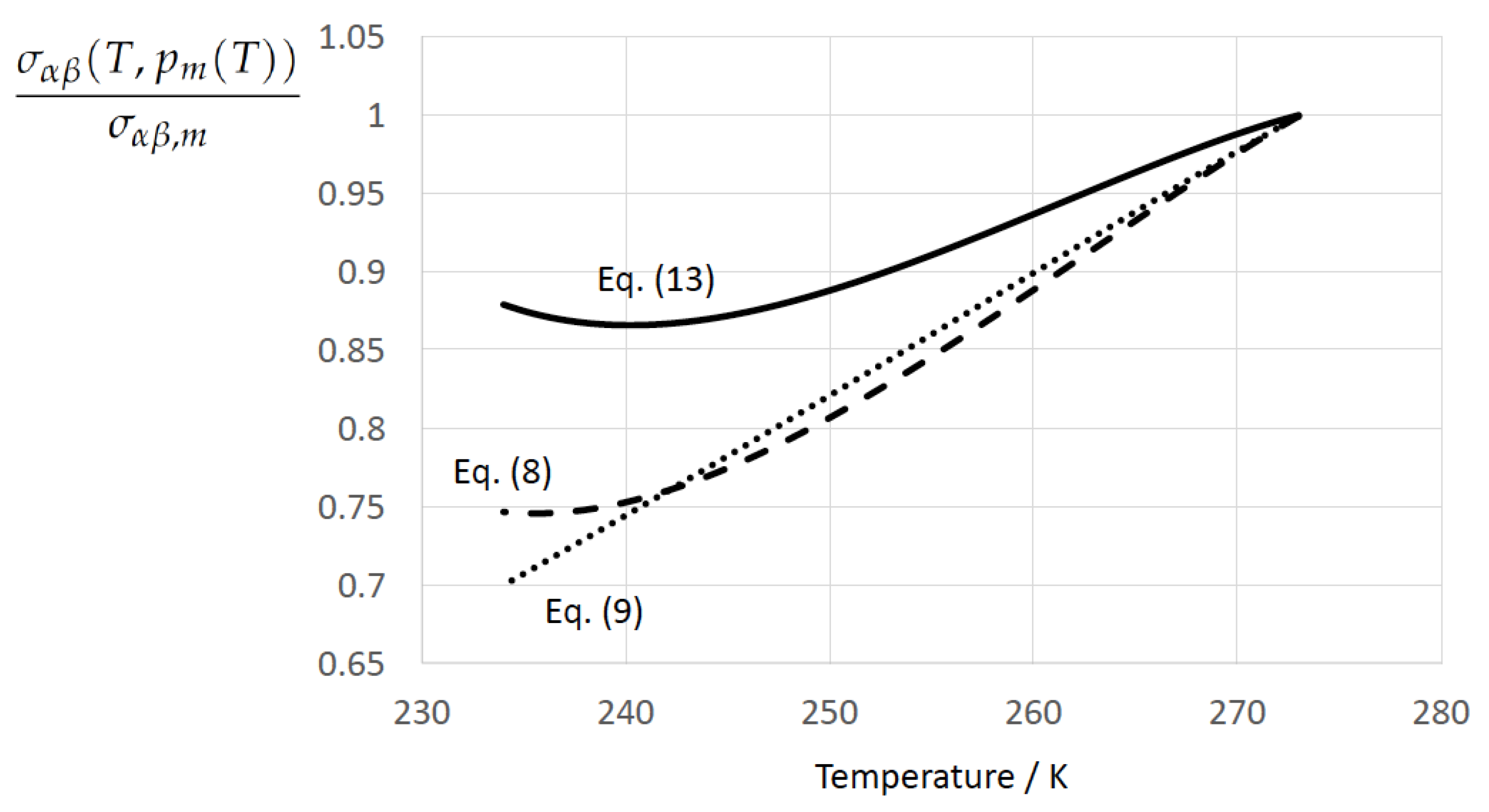
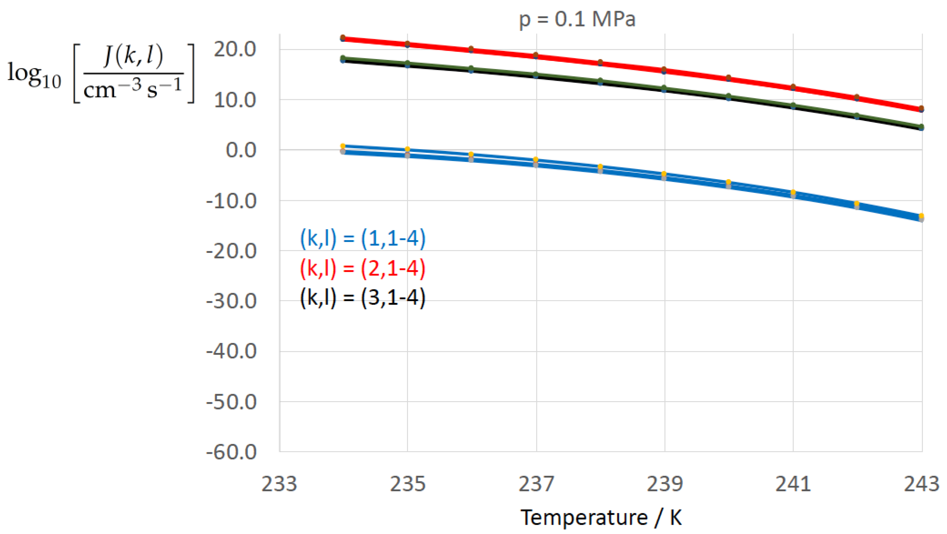
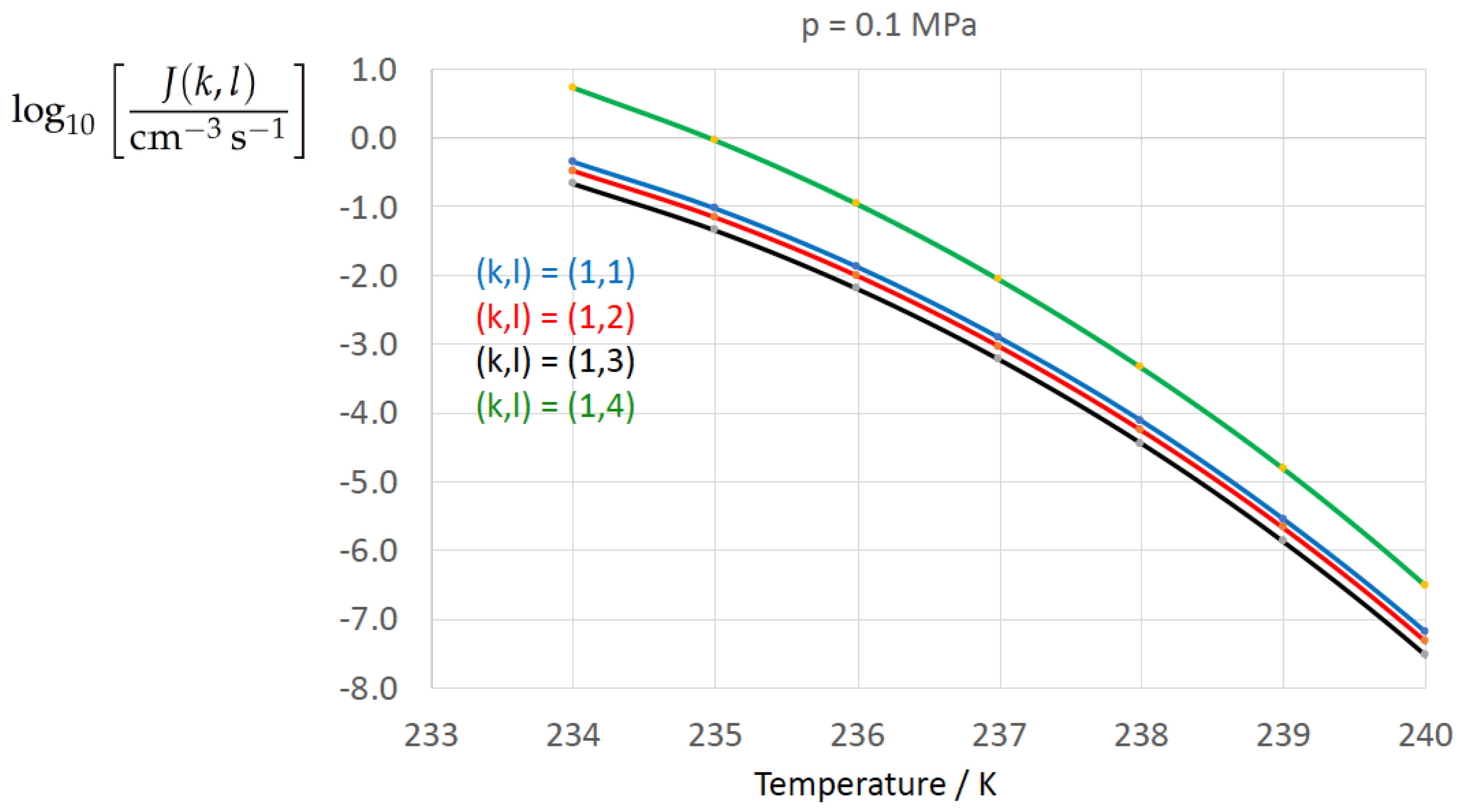
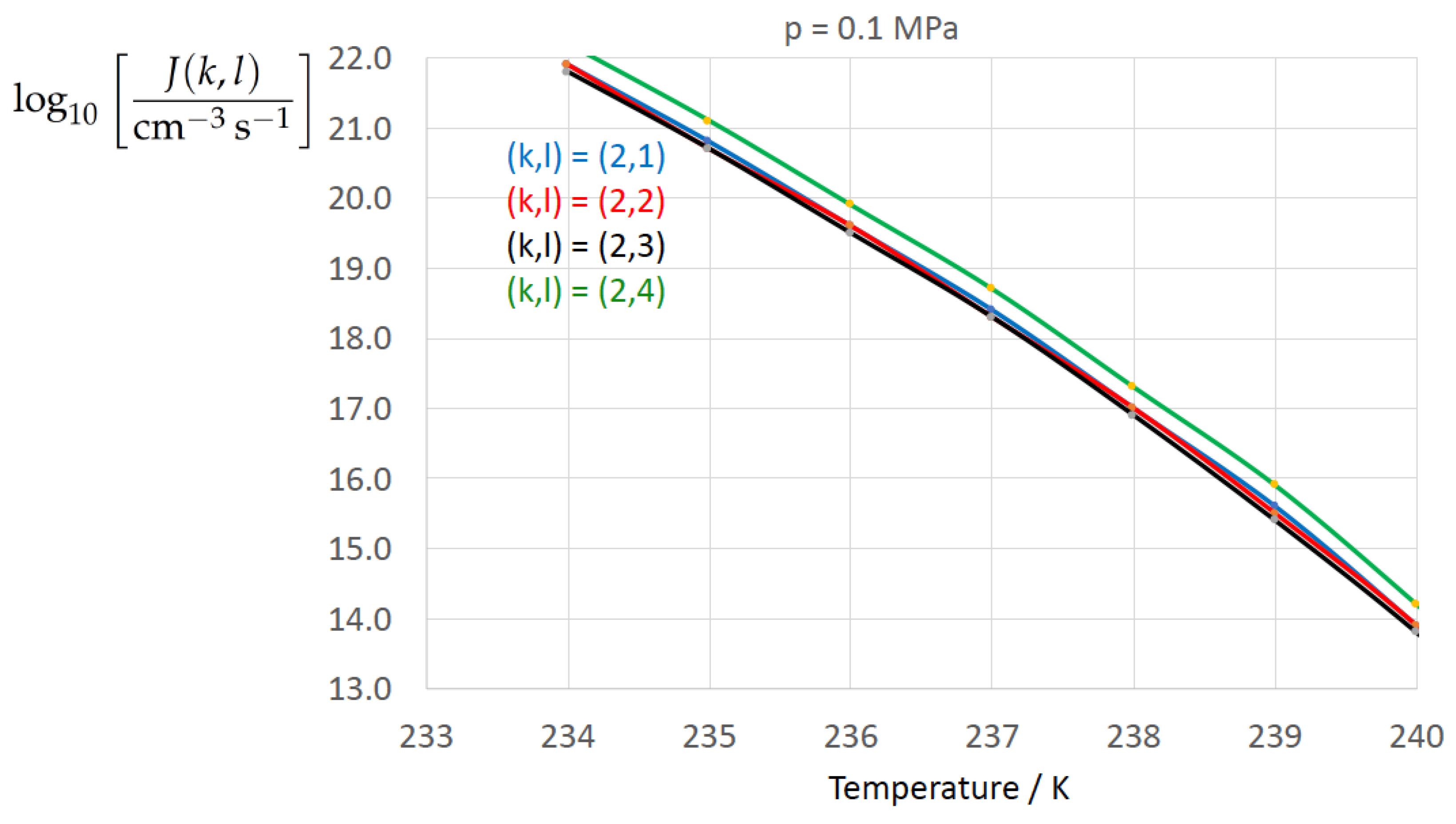
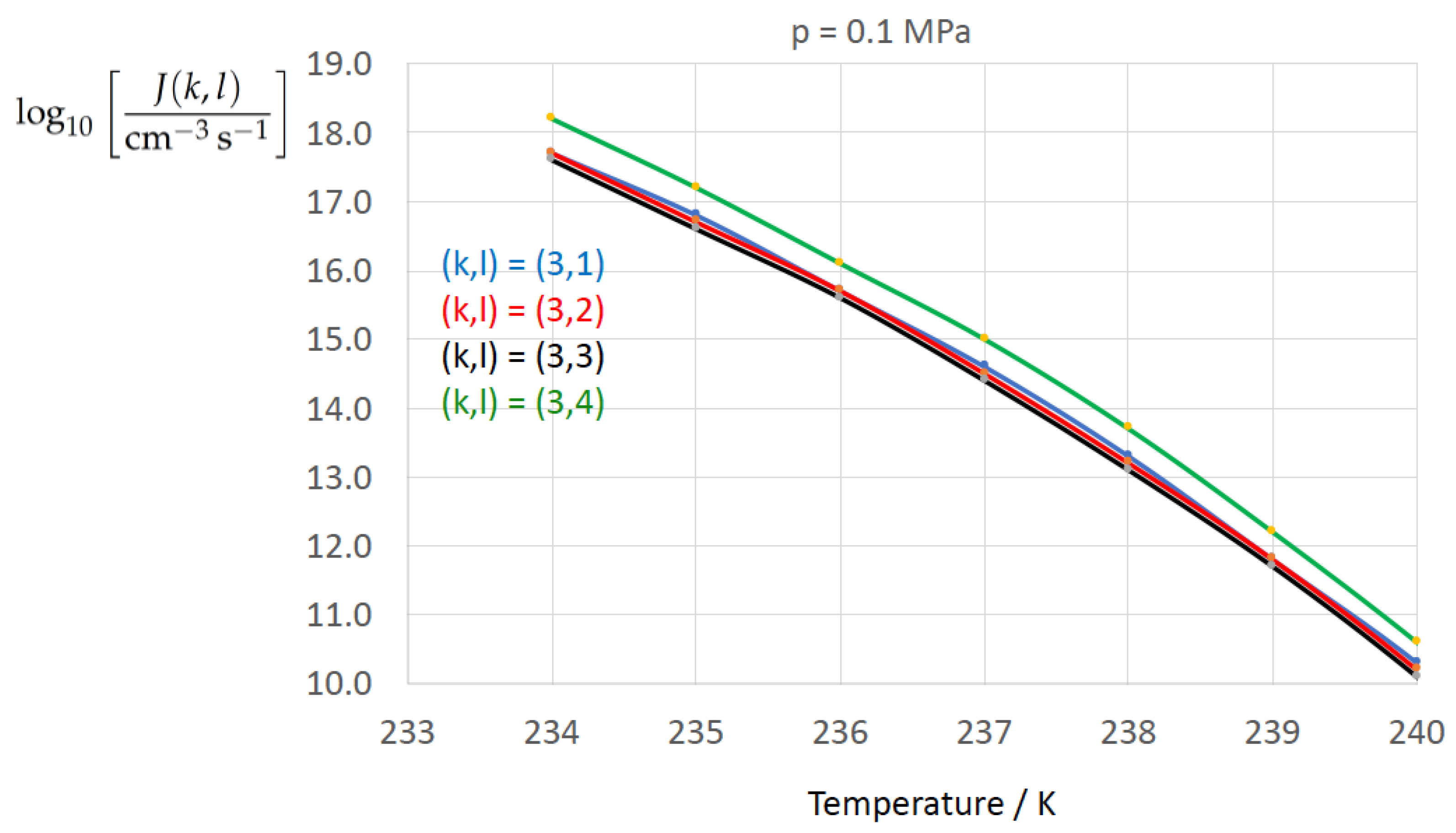
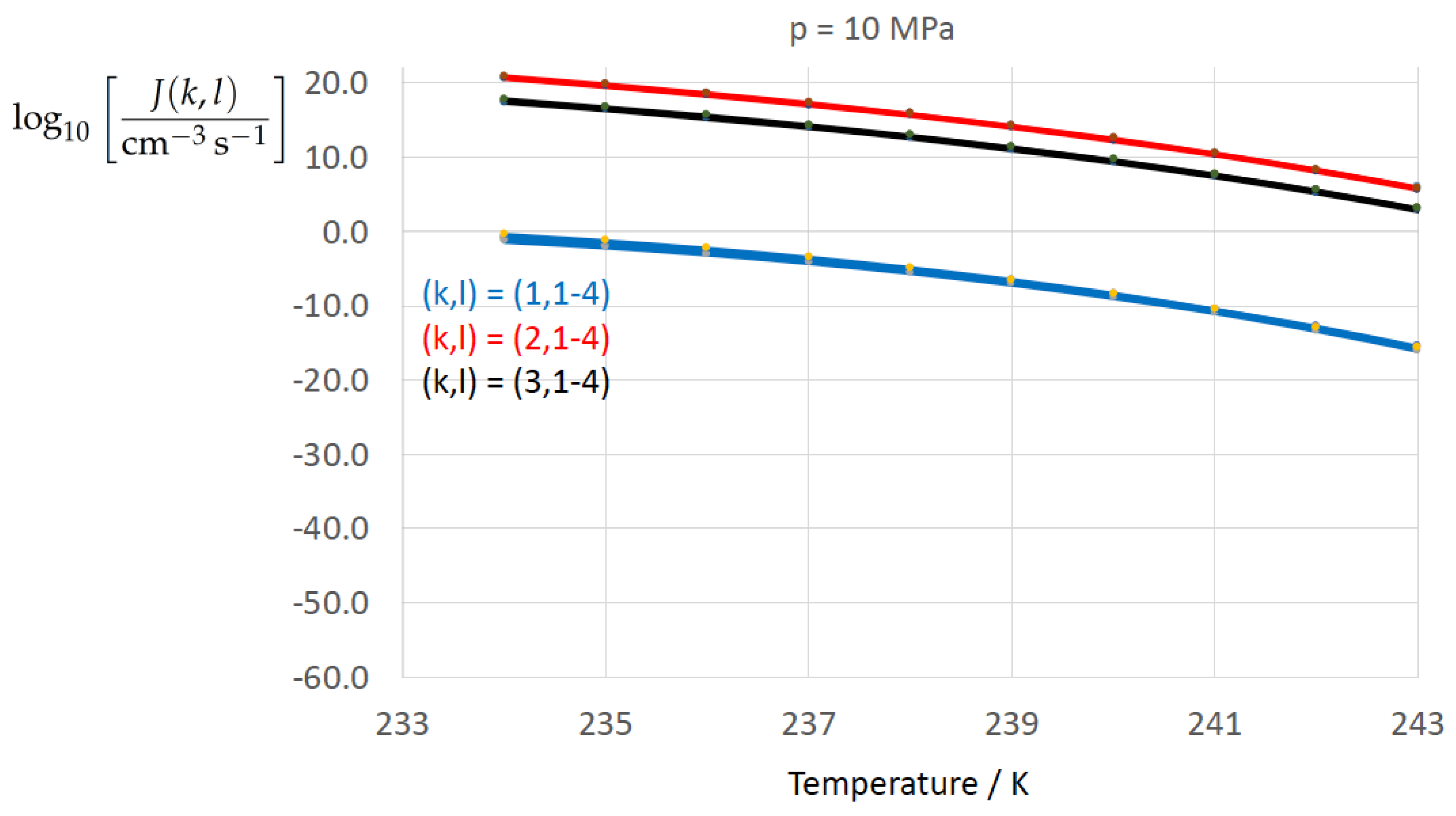
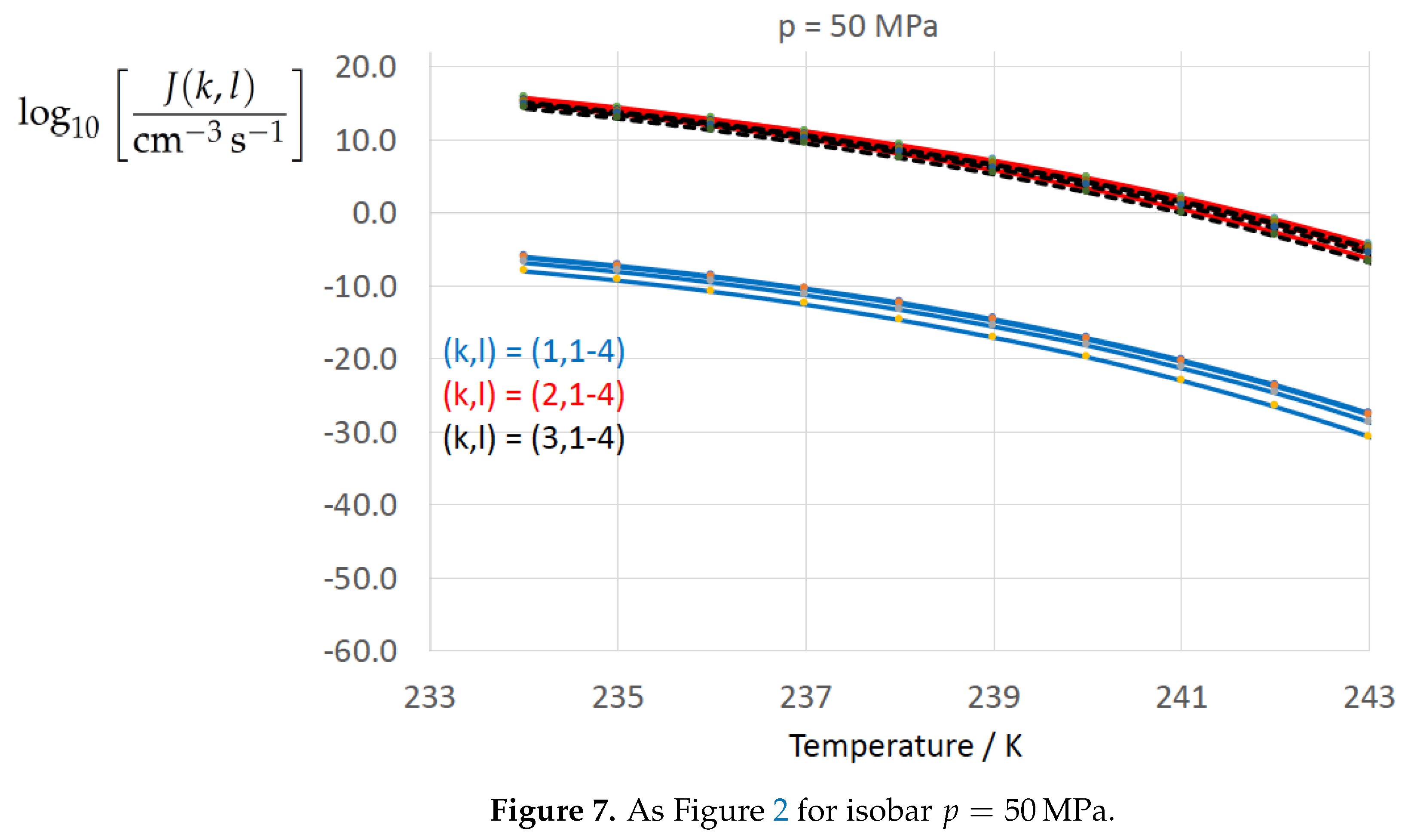
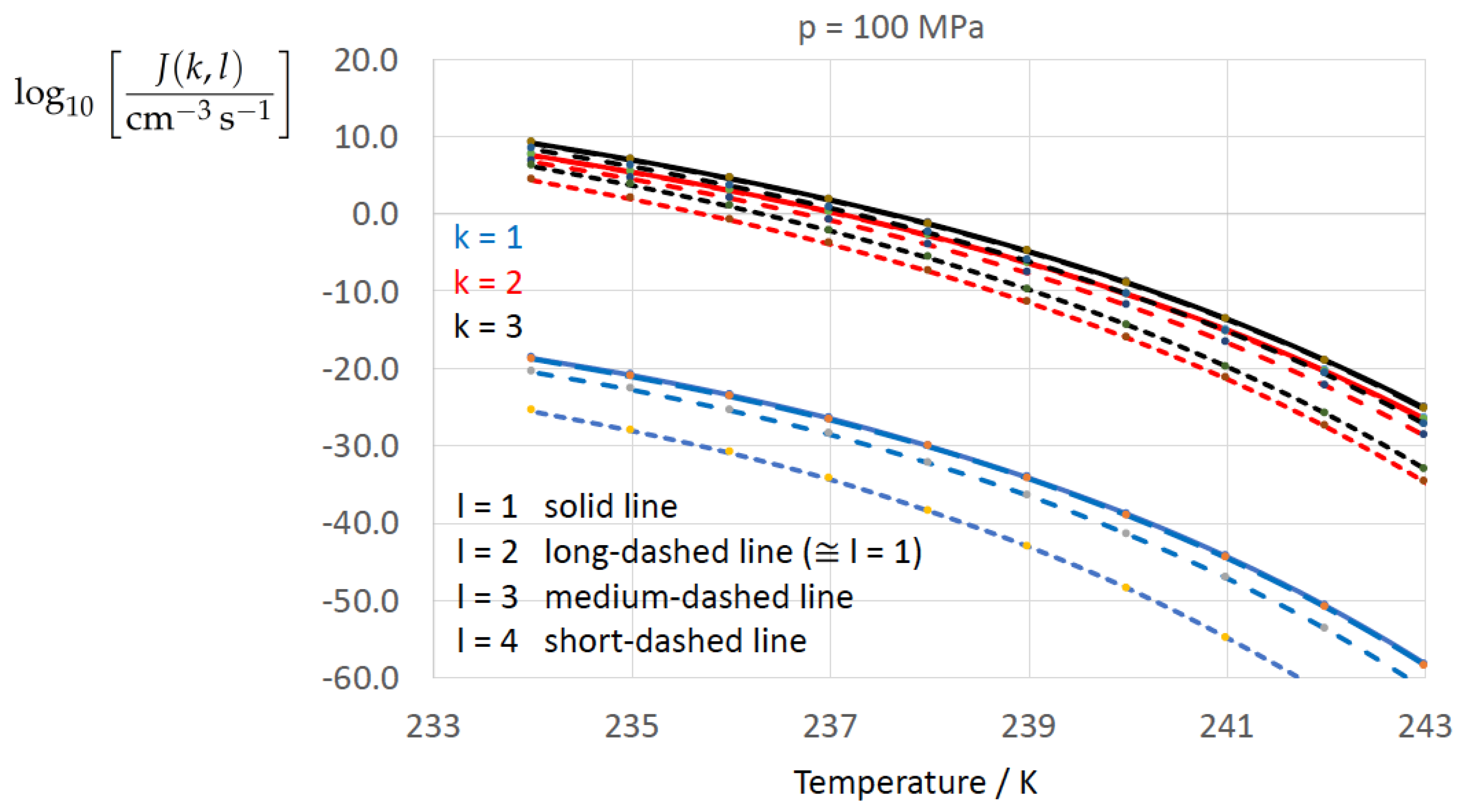
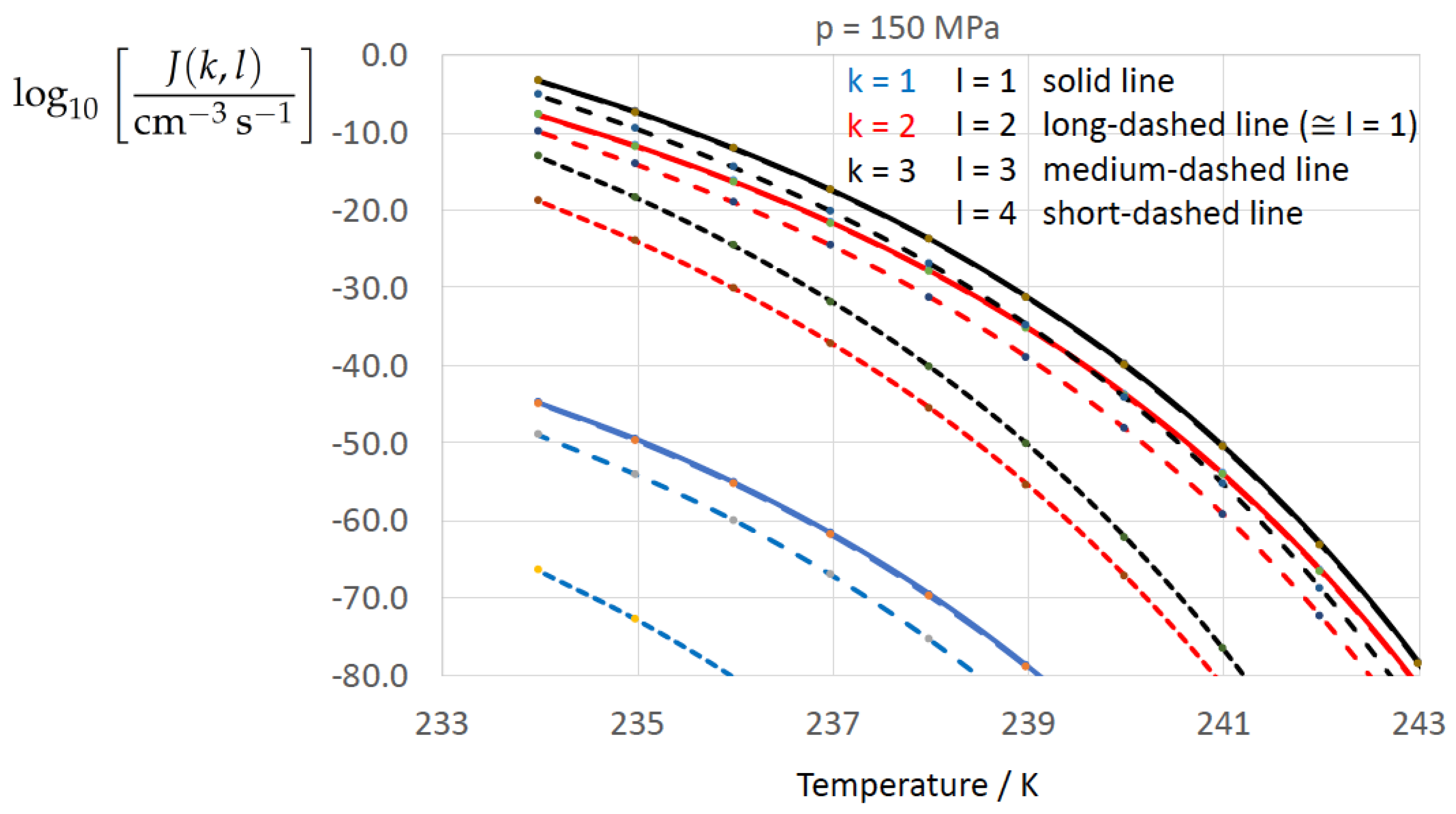
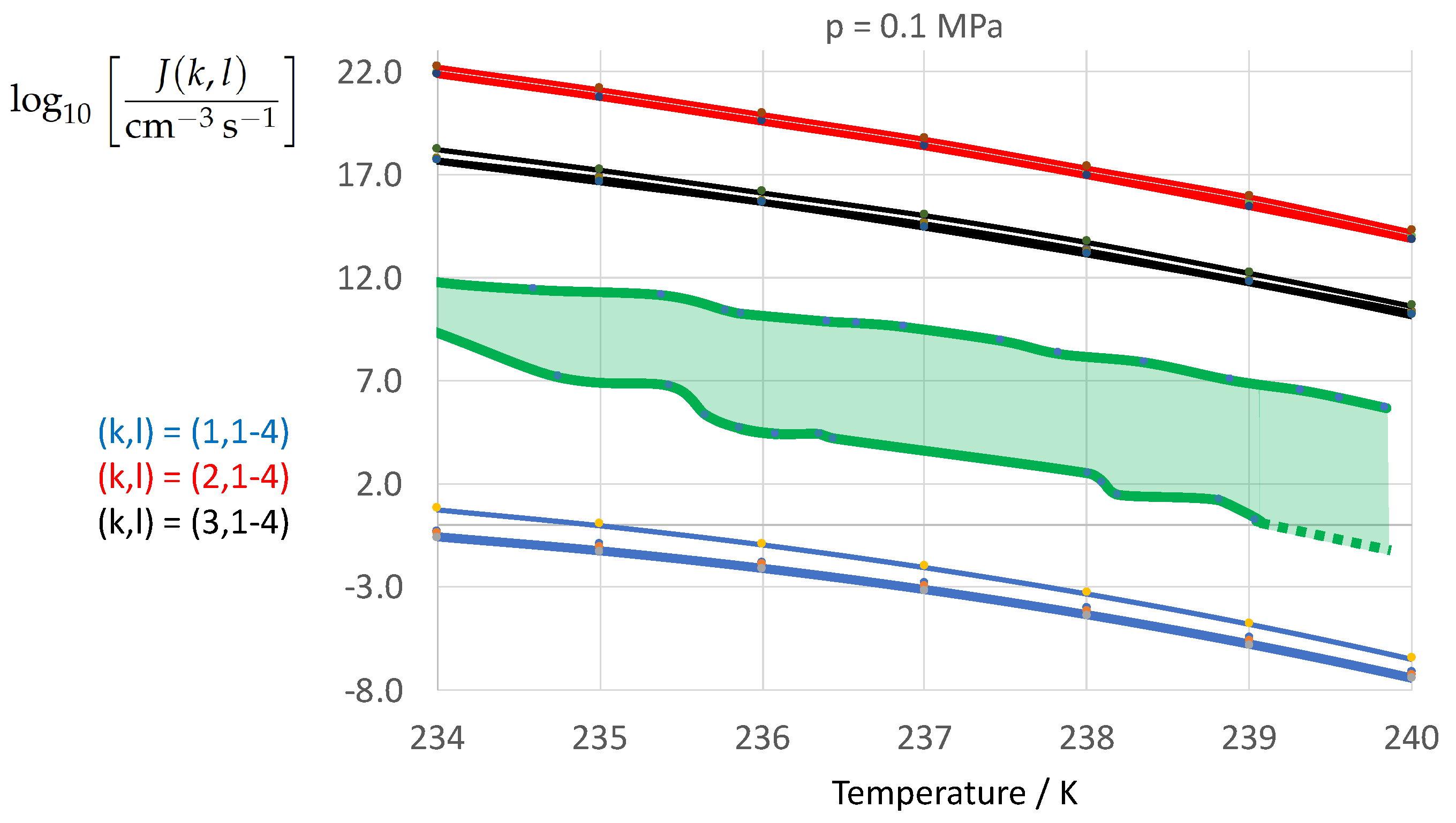
Table A1.
Best fit parameters for the description of the isobaric temperature dependence of in according to Equation (A59). The data in the pressure range were employed by Jeffery and Austin [31] (Table 2). Example: . Taken from Prielmeier et al. [140] (Table 3).
| 347 | 177 | ||
| 10 | 455 | 161 | |
| 50 | 563 | 143 | |
| 100 | 622 | 133 | |
| 150 | 668 | 126 | |
| 200 | 614 | 131 | |
| 250 | 564 | 137 | |
| 300 | 514 | ||
| 350 | 423 | 152 | |
| 400 | 410 |
To estimate , Jeffery and Austin [31] used a separate dataset of self-diffusivity measurements conducted by Harris and Woolf [146] in the temperature and pressure ranges and . Harris and Woolf [146] (Equation (1) and Table 3) derived the following parameterization for :
Table A2.
Best fit parameters for the description of the pressure and temperature dependence of D in according to Equation (A60). Taken from Harris and Woolf [146] (Table 3).
| Value | Value | ||||
|---|---|---|---|---|---|
| = | |||||
| = | = | ||||
| = | = | ||||
| = | = | 0 | |||
| = | |||||
| = | |||||
| = | 0 |
Assuming that at constant pressure is nearly independent of temperature in the considered temperature range, Jeffery and Austin [31] fitted the first relation in Equation (A58) to the data of Harris and Woolf [146]. The fit returned both and the average activation energy .
We checked the values of and derived by Jeffery and Austin [31] by comparison with the predictions from Equation (A60), and identified in this way a mistake in the order of magnitude of presented in Jeffery and Austin [31] (Table 2). Therefore, the correct values are listed here in Table A3.
Finally, inserting from Equation (A59) into Equation (A58) yields the expression for the activation energy proposed by Jeffery and Austin [31] (Equation (15)):
We recalculated the isobars vs. T presented in Jeffery and Austin [31] (figure 4) and found them to be correct. The plot reveals an increase in the activation energy upon increasing undercooling (corresponding to a kinetically controlled nucleation rate depression), and a decrease in the activation energy upon increasing pressure (kinetically controlled nucleation rate enhancement). As the values of both and were subject to the same wrong unit prefactor in Jeffery and Austin [31] (Table 2), the errors (typo) cancel out in the ratio , which enters the activation energy expression, Equation (A61).
References
- Meyers, M.P.; DeMott, P.J.; Cotton, W.R. New primary ice-nucleation parameterizations in an explicit cloud model. J. Appl. Meteorol. 1992, 31, 708–721. [Google Scholar] [CrossRef] [Green Version]
- Khvorostyanov, V.I.; Sassen, K. Toward the theory of homogeneous ice nucleation and its parameterization for cloud models. Geophys. Res. Lett. 1998, 25, 3155–3158. [Google Scholar] [CrossRef]
- Lohmann, U.; Kärcher, B. First interactive simulations of cirrus clouds formed by homogeneous freezing in the ECHAM general circulation model. J. Geophys. Res. 2002, 107. [Google Scholar] [CrossRef]
- Lohmann, U.; Kärcher, B.; Timmreck, C. Impact of the Mount Pinatubo eruption on cirrus clouds formed by homogeneous freezing in the ECHAM4 GCM. J. Geophys. Res. 2003, 108. [Google Scholar] [CrossRef] [Green Version]
- Pruppacher, H.R.; Klett, J.D. Microphysics of Clouds and Precipitation; Kluwer Academic Publishers: Dordrecht, The Netherlands; Boston, MA, USA; London, UK, 2004; 954p. [Google Scholar]
- Heymsfield, A.J.; Miloshevich, L.M.; Schmitt, C.; Bansemer, A.; Twohy, C.; Poellot, M.R.; Fridlind, A.; Gerber, H. Homogeneous ice nucleation in suptropical and tropical convection and its influence on cirrus anvil microphysics. J. Atmos. Sci. 2005, 62, 41–64. [Google Scholar] [CrossRef] [Green Version]
- Jensen, E.J.; Ackerman, A.S. Homogeneous aerosol freezing in the tops of high-altitude tropical cumulonimbus clouds. Geophys. Res. Lett. 2006, 33, L08802. [Google Scholar] [CrossRef]
- Barahona, D.; Nenes, A. Parameterization of cirrus cloud formation in large-scale models: Homogeneous nucleation. J. Geophys. Res. 2008, 113, D11211. [Google Scholar] [CrossRef]
- Jensen, E.J.; Pfister, L.; Bui, T.V.; Lawson, P.; Baker, B.; Mo, Q.; Baumgardner, D.; Weinstock, E.M.; Smith, J.B.; Moyer, E.J.; et al. Formation of large (≃100μm) ice crystals near the tropical tropopause. Atmos. Chem. Phys. 2008, 8, 1621–1633. [Google Scholar] [CrossRef] [Green Version]
- Zasetsky, A.Y.; Petelina, S.V.; Svishchev, I.M. Thermodynamics of homogeneous nucleation of ice particles in the polar summer mesosphere. Atmos. Chem. Phys. 2009, 9, 965–971. [Google Scholar] [CrossRef] [Green Version]
- Khvorostyanov, V.I.; Curry, J.A. Critical humidities of homogeneous and heterogeneous ice nucleation: Inferences from extended classical nucleation theory. J. Geophys. Res. 2009, 114, D04307. [Google Scholar] [CrossRef]
- Khvorostyanov, V.I.; Curry, J.A. Parameterization of homogeneous ice nucleation for cloud and climate models based on classical nucleation theory. Atmos. Chem. Phys. 2012, 12, 9275–9302. [Google Scholar] [CrossRef] [Green Version]
- Hellmuth, O.; Khvorostyanov, V.I.; Curry, J.A.; Shchekin, A.K.; Schmelzer, J.W.P.; Feistel, R.; Djikaev, Y.S.; Baidakov, V.G. Selected aspects of atmospheric ice and salt crystallisation. In Nucleation Theory and Applications; Schmelzer, J.W.P., Hellmuth, O., Eds.; JINR Joint Institute for Nuclear Research, Bogoliubov Laboratory of Theoretical Physics: Dubna, Russia, 2013; Volume 1, p. 513. ISBN 978-5-9530-0349-0. [Google Scholar]
- Khvorostyanov, V.I.; Curry, J.A. Thermodynamics, Kinetics, and Microphysics of Clouds, 1st ed.; Cambridge University Press: Cambridge, UK, 2014; p. 782. [Google Scholar]
- Lohmann, U.; Lüönd, F.; Mahrt, F. An Introduction to Clouds. From Microscale to Climate; Cambridge University Press: Cambridge, UK, 2016. [Google Scholar]
- Pegg, D.E. Principles of Cryopreservation. In Cryopreservation and Freeze-Drying Protocols. Methods in Molecular Biology; Day, J.G., Stacey, G.N., Eds.; Humana Press Inc.: Totowa, NJ, USA, 2007; Volume 368. [Google Scholar]
- Espinosa, J.R.; Sanz, E.; Valeriani, C.; Vega, C. Homogeneous ice nucleation evaluated for several water models. J. Chem. Phys. 2014, 141, 180529. [Google Scholar] [CrossRef] [PubMed] [Green Version]
- Espinosa, J.R.; Zaragoza, A.; Rosales-Pelaez, P.; Navarro, C.; Valeriani, C.; Vega, C.; Sanz, E. Interfacial free energy as the key to the pressure-induced deceleration of ice nucleation. Phys. Rev. Lett. 2016, 117, 135702. [Google Scholar] [CrossRef] [PubMed]
- Debenedetti, P.G.; Stanley, H.E. Supercooled and glassy water. Phys. Today 2003, 56, 40–46. [Google Scholar] [CrossRef]
- Bhat, S.N.; Sharma, A.; Bhat, S.V. Vitrification and Glass Transition of Water: Insights from Spin Probe ESR. Phys. Rev. Lett. 2005, 95, 235702. [Google Scholar] [CrossRef] [PubMed] [Green Version]
- Zobrist, B.; Marcolli, C.; Pedernera, D.A.; Koop, T. Do atmospheric aerosols form glasses? Atmos. Chem. Phys. 2008, 8, 5221–5244. [Google Scholar] [CrossRef] [Green Version]
- McDonald, J.E. Homogeneous nucleation of supercooled water drops. J. Meteorol. 1953, 10, 416–433. [Google Scholar] [CrossRef] [Green Version]
- Butorin, G.T.; Skripov, V.P. Crystallization of supercooled water. Kristallografiya 1972, 17, 379–384. [Google Scholar]
- Hagen, D.E.; Anderson, R.J.; Kassner, J.L. Homogeneous condensation–freezing nucleation rate measurements for small water droplets in an expansion cloud chamber. J. Atmos. Sci. 1981, 38, 1236–1243. [Google Scholar] [CrossRef] [Green Version]
- Hare, D.E.; Sorensen, C.M. The density of supercooled water. II. Bulk samples cooled to the homogeneous nucleation limit. J. Chem. Phys. 1987, 87, 4840–4845. [Google Scholar] [CrossRef]
- Henderson, S.J.; Speedy, R.J. Melting temperature of ice at positive and negative pressures. J. Phys. Chem. 1987, 91, 3069–3072. [Google Scholar] [CrossRef]
- Speedy, J.R. Thermodynamic properties of supercooled water at 1 atm. J. Phys. Chem. 1987, 91, 3354–3358. [Google Scholar] [CrossRef]
- Bartell, L.S.; Huang, J. Supercooling of water below the anomalous range near 226K. J. Phys. Chem. 1994, 98, 7455–7457. [Google Scholar] [CrossRef]
- Gránásy, L. Diffuse interface analysis of ice nucleation in undercooled water. J. Phys. Chem. 1995, 99, 14182–14187. [Google Scholar] [CrossRef]
- Huang, J.; Bartell, L.S. Kinetics of homogeneous nucleation in the freezing of large water clusters. J. Phys. Chem. 1995, 99, 3924–3931. [Google Scholar] [CrossRef]
- Jeffery, C.A.; Austin, P.H. Homogeneous nucleation of supercooled water: Results from a new equation state. J. Geophys. Res. 1997, 102, 25269–25279. [Google Scholar] [CrossRef]
- Benz, S.; Megahed, K.; Möhler, O.; Saathoff, H.; Wagner, R.; Schurath, U. T-dependent rate measurements of homogeneous ice nucleation in cloud droplets using a large atmospheric simulation chamber. J. Photochem. Photobiol. A Chem. 2005, 176, 208–217. [Google Scholar] [CrossRef]
- Holten, V.; Labetski, D.G.; van Dongen, M.E.H. Homogeneous nucleation of water between 200 and 240 K: New wave tube data and estimation of Tolman length. J. Chem. Phys. 2005, 123, 104505. [Google Scholar] [CrossRef] [Green Version]
- Stöckel, P.; Weidinger, I.M.; Baumgärtel, H.; Leisner, T. Rates of homogeneous ice nucleation in levitated H2O and D2O droplets. J. Phys. Chem. A 2005, 109, 2540–2546. [Google Scholar] [CrossRef]
- Souda, R. Liquid-liquid transition in supercooled water investigated by interaction with LiCl and Xe. J. Chem. Phys. 2006, 125, 181103. [Google Scholar] [CrossRef]
- Tabazadeh, A.; Djikaev, Y.S.; Reiss, H. Surface crystallization of supercooled water in clouds. PNAS 2002, 99, 15873–15878. [Google Scholar] [CrossRef] [PubMed] [Green Version]
- Vortisch, H.; Krämer, B.; Weidinger, I.; Wöste, L.; Leisner, T.; Schwell, M.; Baumgärtel, H.; Rühl, E. Homogeneous freezing nucleation rates and crystallization dynamics of single levitated sulfuric acid solution droplets. Phys. Chem. Chem. Phys. 2000, 2, 1407–1413. [Google Scholar] [CrossRef]
- Malila, J.; Laaksonen, A. Properties of Supercooled Water Clusters from Nucleation Rate Data with the Effect of Non-Ideal Vapour Phase. In Proceedings of the Preprint—ICPWS XV, Berlin, Germany, 8–11 September 2008. [Google Scholar]
- Atkinson, J.D.; Murray, B.J.; O’Sullivan, D. Rate of homogeneous nucleation of ice in supercooled water. J. Phys. Chem. A 2016, 120, 6513–6520. [Google Scholar] [CrossRef] [PubMed] [Green Version]
- Gránásy, L. Cahn-Hilliard-type density functional calculations for homogeneous ice nucleation in undercooled water. J. Mol. Struct. 1999, 485–486, 523–536. [Google Scholar] [CrossRef]
- Matsumoto, M.; Saito, S.; Ohmine, I. Molecular dynamics simulation of the ice nucleation and growth process leading to water freezing. Nature 2002, 416, 409–413. [Google Scholar] [CrossRef] [PubMed]
- Oxtoby, D.W. Crystal nucleation in simple and complex fluids. Phil. Trans. R. Soc. Lond. A 2003, 361, 419–428. [Google Scholar] [CrossRef]
- Nada, H.; van der Eerden, J.P.; Furukawa, Y. A clear observation of crystal growth of ice from water in a molecular dynamics simulation with a six-site potential model of H2O. J. Cryst. Growth 2004, 266, 297–302. [Google Scholar] [CrossRef] [Green Version]
- Laird, B.B.; Davidchack, R.L. Direct calculation of the crystal-melt interfacial free energy via molecular dynamics computer simulation. J. Phys. Chem. B 2005, 109, 17802–17812. [Google Scholar] [CrossRef]
- Vega, C.; Abascal, J.L.F. Relation between the melting temperature and the temperature of maximum density for the most common models of water. J. Chem. Phys. 2005, 123, 144504. [Google Scholar] [CrossRef] [Green Version]
- Bai, X.M.; Li, M. Calculation of solid-liquid interfacial free energy: A classical nucleation theory based approach. J. Chem. Phys. 2006, 124, 124707. [Google Scholar] [CrossRef]
- Bartell, L.S.; Wu, D.T. A new prodecure for analyzing the nucleation kinetics of freezing in computer simulation. J. Chem. Phys. 2006, 125, 194503. [Google Scholar] [CrossRef] [PubMed] [Green Version]
- Hernández de la Peña, L.; Kusalik, P.G. Quantum effects in liquid water and ice: Model dependence. J. Chem. Phys. 2006, 125, 054512. [Google Scholar] [CrossRef] [Green Version]
- Vega, C.; Abascal, J.L.F.; Nezbeda, I. Vapor-liquid equilibria from the triple point up to the critical point for the new generation of TIP4P-like models: TIP4P/Ew, TIP4P/2005, and TIP4P/ice. J. Chem. Phys. 2006, 125, 034503. [Google Scholar] [CrossRef] [PubMed]
- Vrbka, L.; Jungwirth, P. Homogeneous freezing of water starts in the subsurface. J. Phys. Chem. B 2006, 110, 18126–18129. [Google Scholar] [CrossRef] [PubMed]
- Moore, E.B.; Molinero, V. Structural transformation in supercooled water controls the crystallization rate of ice. Nature 2011, 479, 506–509. [Google Scholar] [CrossRef] [PubMed]
- Tanaka, K.K.; Kimura, Y. Theoretical analysis of crystallization by homogeneous nucleation of water droplets. Phys. Chem. Chem. Phys. 2019, 21, 2410–2418. [Google Scholar] [CrossRef] [PubMed] [Green Version]
- Bartell, L.S. Nucleation rates in freezing and solid-state transitions. Molecular clusters as model systems. J. Phys. Chem. 1995, 99, 1080–1089. [Google Scholar] [CrossRef]
- Ford, I.J. Properties of ice clusters from an analysis of freezing nucleation. J. Phys. Chem. B 2001, 105, 11649–11655. [Google Scholar] [CrossRef]
- Debenedetti, P.G. Supercooled and glassy water. J. Phys. Condens. Matter 2003, 15, R1669–R1726. [Google Scholar] [CrossRef] [Green Version]
- Ludwig, R. Wasser: Von Clustern in die Flüssigkeit. Angew. Chem. 2001, 113, 1856–1876. [Google Scholar] [CrossRef]
- Skripov, V.P. Metastable Liquids; John Wiley & Sons: New York, NY, USA, 1974. [Google Scholar]
- Skripov, V.P.; Baidakov, V.G. Pereohlaždennaâ židkost’—Otsutctvie spinodali. Teplofiz. Vysok. Temp. 1972, 10, 1226–1230. [Google Scholar]
- Skripov, V.P.; Koverda, V.P. Spontaneous Crystallization of Undercooled Liquids; Nauka: Moscow, Russia, 1984. (In Russian) [Google Scholar]
- Debenedetti, P.G.; Raghavan, V.S.; Borick, S.S. Spinodal curve of some supercooled liquids. J. Phys. Chem. 1991, 95, 4540–4551. [Google Scholar] [CrossRef]
- Baidakov, V.G. Peregrev Kriogennyh Židkostej; UrO RAN: Ekaterinburg, Russia, 1995; p. 264. [Google Scholar]
- Baidakov, V.G. Experimental investigations of superheated and supercooled water (review of papers of the school of the Academician V. P. Skripov). In Proceedings of the 15th International Conference on the Properties of Water and Steam, Conference Proceedings, Preprint ICPWS XV, Berlin, Germany, 8–11 September 2008. [Google Scholar]
- Baidakov, V.G. Temperature dependence of the surface free energy of a crystal-liquid interface. Russ. J. Phys. Chem. A 2012, 86, 1763–1765. [Google Scholar] [CrossRef]
- Baidakov, V.G. Crystallization of Undercooled Liquids: Results of Molecular Dynamics Simulations. In Glass: Selected Properties and Crystallization; Schmelzer, J.W.P., Ed.; de Gruyter: Berlin, Germany; Boston, MA, USA, 2014; pp. 481–520. [Google Scholar]
- Baidakov, V.G.; Protsenko, S.P. Singular point of a system of Lennard-Jones particles at negative pressure. Phys. Rev. Lett. 2005, 95, 015701. [Google Scholar] [CrossRef] [PubMed]
- Baidakov, V.G.; Protsenko, S.P. Molecular-dynamics investigation of phase equilibrium and surface tension in argon–neon system. J. Phys. Chem. C 2008, 112, 17231–17234. [Google Scholar] [CrossRef]
- Skripov, V.P.; Faizullin, M.Z. Crystal-Liquid-Gas Phase Transitions and Thermodynamic Similarity; WILEY-VCH Verlag GmbH & Co. KGaA: Weinheim, Germany, 2006. [Google Scholar]
- Baidakov, V.G.; Protsenko, S.P.; Kozlova, Z.R.; Chernykh, G.G. Metastable extension of the liquid-vapor phase equilibrium curve and surface tension. J. Chem. Phys. 2007, 126, 214505. [Google Scholar] [CrossRef]
- Bartell, L.S.; Wu, D.T. Do supercooled liquids freeze by spinodal decomposition? J. Chem. Phys. 2007, 127, 174507. [Google Scholar] [CrossRef]
- Wagner, W.; Pruß, A. The IAPWS formulation 1995 for the thermodynamic properties of ordinary water substance for general and scientific use. J. Phys. Chem. Ref. Data 2002, 31, 387–535. [Google Scholar] [CrossRef] [Green Version]
- Wagner, W.; Riethmann, T.; Feistel, R.; Harvey, A.H. New equations for the sublimation pressure and melting pressure of H2O ice Ih. J. Phys. Chem. Ref. Data 2011, 40, 043103. [Google Scholar] [CrossRef] [Green Version]
- Guder, C. FORTRAN Implementation of the IAPWS Release on an Equation of State for H2O Ice Ih ([email protected], Code Version: 22 June 2006); Technical Report; International Association for the Properties of Water and Steam: Witney, UK, 2006. [Google Scholar]
- Feistel, R.; Hagen, E. On the Gibbs thermodynamic potential of seawater. Progr. Oceanogr. 1995, 36, 249–327. [Google Scholar] [CrossRef]
- Feistel, R. A new extended Gibbs thermodynamic potential of seawater. Prog. Oceanogr. 2003, 58, 43–114. [Google Scholar] [CrossRef]
- Feistel, R. A Gibbs function for seawater thermodynamics for −6 to 80 °C and salinity up to 120g kg−1. Deep-Sea Res. I 2008, 55, 1639–1671. [Google Scholar] [CrossRef]
- Feistel, R.; Wright, D.G.; Miyagawa, K.; Harvey, A.H.; Hruby, J.; Jackett, D.R.; McDougall, T.J.; Wagner, W. Mutually consistent thermodynamic potentials for fluid water, ice and seawater: A new standard for oceanography. Ocean Sci. 2008, 4, 275–291. [Google Scholar] [CrossRef] [Green Version]
- Feistel, R.; Hagen, E. A Gibbs thermodynamic potential of sea ice. Cold Reg. Sci. Technol. 1998, 28, 83–142. [Google Scholar] [CrossRef]
- Feistel, R.; Hagen, E. Corrigendum to “A Gibbs thermodynamic potential of sea ice”. Cold Reg. Sci. Technol. 1999, 29, 173–176. [Google Scholar]
- Feistel, R.; Wagner, W. A Comprehensive Gibbs Potential of Ice. In Water, Steam, and Aqueous Solutions for Electric Power; Nakahara, M., Matubayasi, N., Ueno, M., Yasuoka, K., Watanabe, K., Eds.; MARUZEN Co., Ltd.: Tokyo, Japan, 2005; pp. 751–756. [Google Scholar]
- Feistel, R.; Wagner, W. A Comprehensive Gibbs Potential of Ice Ih. In Nucleation Theory and Applications; Schmelzer, J.W.P., Röpke, G., Priezzhev, V.B., Eds.; JINR Joint Institute for Nuclear Research, Bogoliubov Laboratory of Theoretical Physics: Dubna, Russia, 2005; pp. 120–145. ISBN 5-9530-0098-7. [Google Scholar]
- Feistel, R.; Wagner, W. High-pressure thermodynamic Gibbs functions of ice and sea ice. J. Mar. Res. 2005, 63, 95–139. [Google Scholar] [CrossRef]
- Feistel, R.; Wagner, W. A new equation of state for H2O ice Ih. J. Phys. Chem. Ref. Data 2006, 35, 1021–1047. [Google Scholar] [CrossRef] [Green Version]
- IAPWS R10-06. Revised Release on the Equation of State 2006 for H2O Ice Ih; Technical Report; The International Association for the Properties of Water and Steam: Doorwerth, The Netherlands, September 2009. [Google Scholar]
- Holten, V.; Bertrand, C.E.; Anisimov, M.A.; Sengers, J.V. Thermodynamic Modeling of Supercooled Water. Technical Report for The International Association for the Properties of Water and Steam (IAPWS) (September 2011); Technical Report; Institute for Physical Science and Technology and Department of Chemical and Biomolecular Engineering, University of Maryland: College Park, MD, USA, 2011. [Google Scholar]
- Holten, V.; Bertrand, C.E.; Anisimov, M.A.; Sengers, J.V. Thermodynamics of supercooled water. J. Chem. Phys. 2012, 136, 094507. [Google Scholar] [CrossRef] [Green Version]
- Holten, V.; Sengers, J.V.; Anisimov, M.A. Equation of state for supercooled water at pressures up to 400 MPa. J. Phys. Chem. Ref. Data 2014, 43, 043101. [Google Scholar] [CrossRef] [Green Version]
- Feistel, R.; Wright, D.G.; Jackett, D.R.; Miyagawa, K.; Reissmann, J.H.; Wagner, W.; Overhoff, U.; Guder, C.; Feistel, A.; Marion, G.M. Numerical implementation and oceanographic application of the thermodynamic potentials of liquid water, water vapour, ice, seawater and humid air–Part 1: Background and equations. Ocean Sci. 2010, 6, 633–677. [Google Scholar] [CrossRef] [Green Version]
- Wright, D.G.; Feistel, R.; Reissmann, J.H.; Miyagawa, K.; Jackett, D.R.; Wagner, W.; Overhoff, U.; Guder, C.; Feistel, A.; Marion, G.M. Numerical implementation and oceanographic application of the thermodynamic potentials of liquid water, water vapour, ice, seawater and humid air—Part 2: The library routines. Ocean Sci. 2010, 6, 695–718. [Google Scholar] [CrossRef] [Green Version]
- Feistel, R. TEOS-10: A new international oceanographic standard for seawater, ice, fluid water and humid air. Int. J. Thermophys. 2012, 33, 1335–1351. [Google Scholar] [CrossRef]
- Feistel, R. Thermodynamic properties of seawater, ice and humid air: TEOS-10, before and beyond. Ocean Sci. 2018, 14, 471–502. [Google Scholar] [CrossRef] [Green Version]
- IAPWS R6-95. Revised Release on the IAPWS Formulation 1995 for the Thermodynamic Properties of Ordinary Water Substance for General and Scientific Use; Technical Report; The International Association for the Properties of Water and Steam: Dresden, Germany, September 2016. [Google Scholar]
- IAPWS. Revised Release on the IAPWS Industrial Formulation 1997 For the Thermodynamic Properties of Water and Steam. (The Revision Only Relates to the Extension of Region 5 to 50 MPa); Technical Report; The International Association for the Properties of Water and Steam: Lucerne, Switzerland, August 2007. [Google Scholar]
- Release on the IAPWS Formulation 2008 for the Thermodynamic Properties of Seawater; Technical Report, IAPWS R13-08; The International Association for the Properties of Water and Steam: Berlin, Germany, September 2008.
- IAPWS. Supplementary Release on a Computationally Efficient Thermodynamic Formulation for Liquid Water for Oceanographic Use; Technical Report; The International Association for the Properties of Water and Steam: Doorwerth, The Netherlands, September 2009. [Google Scholar]
- IAPWS. Guideline on a Low-Temperature Extension of the IAPWS-95 Formulation for Water Vapor; Technical Report; The International Association for the Properties of Water and Steam: Boulder, CO, USA, September/October 2012. [Google Scholar]
- IAPWS G12-15. Guideline on Thermodynamic Properties of Supercooled Water; Technical Report; The International Association for the Properties of Water and Steam: Stockholm, Sweden, July 2015. [Google Scholar]
- McDougall, T.J.; Feistel, R.; Wright, D.G.; Pawlowicz, R.; Millero, F.J.; Jackett, D.R.; King, B.A.; Marion, G.M.; Seitz, S.; Spitzer, P.; et al. The International Thermodynamic Equation of Seawater—2010: Calculation and Use of Thermodynamic Properties; Technical Report; Manuals and Guides No. 56, UNESCO; Intergovernmental Oceanographic Commission: Paris, France, 2010; 196p. (In English) [Google Scholar]
- Gutzow, I.; Schmelzer, J.W.P. The Vitreous State: Thermodynamics, Structure, Rheology, and Crystallization, 1st ed.; Springer: Berlin/Heidelberg, Germany, 1995; 468p. [Google Scholar]
- Gutzow, I.; Schmelzer, J.W.P. The Vitreous State: Thermodynamics, Structure, Rheology, and Crystallization, 2nd ed.; Springer: Berlin/Heidelberg, Germany, 2013; 553p. [Google Scholar]
- Debenedetti, P.G. Metastable Liquids: Concepts and Principles; Princeton University Press: Princeton, NJ, USA, 1996. [Google Scholar]
- Kelton, K.F.; Greer, A.L. Nucleation in Condensed Matter: Applications in Materials and Biology; Pergamon: Amsterdam, The Netherlands, 2010. [Google Scholar]
- Herlach, D.; Galenko, P.; Holland-Moritz, D. Metastable Solids from Undercooled Melts; Pergamon Materials Series; Cahn, R.W., Ed.; Elsevier: Amsterdam, The Netherlands, 2007; Volume 10. [Google Scholar]
- Gibbs, J.W. On the equilibrium of heterogeneous substances. Trans. Connect. Acad. Arts Sci. 1877, III, 44–520. [Google Scholar] [CrossRef]
- Gibbs, J.W. The Scientific Papers of J. W. Gibbs. Vol. 1: Thermodynamics; Dover: New York, NY, USA, 1961. [Google Scholar]
- Schmelzer, J.W.P.; Abyzov, A.S. Crystallization of glass-forming liquids: Thermodynamic driving force. J. Non-Cryst. Solids 2016, 449, 41–49. [Google Scholar] [CrossRef]
- Schmelzer, J.W.P.; Abyzov, A.S.; Fokin, V.M. Crystallization of glass: What we know, what we need to know. Int. J. Appl. Glass Sci. 2016, 7, 253–261. [Google Scholar] [CrossRef]
- Schmelzer, J.W.P.; Abyzov, A.S. Crystallization of glass-forming melts: New answers to old questions. J. Non-Cryst. Solids 2018, 501, 11–20. [Google Scholar] [CrossRef]
- Schmelzer, J.W.P.; Abyzov, A.S. Crystallization of glass-forming liquids: Specific surface energy. J. Chem. Phys. 2016, 145, 064512. [Google Scholar] [CrossRef]
- Schmelzer, J.W.P.; Abyzov, A.S.; Fokin, V.M. Thermodynamic aspects of pressure-induced crystallization: Kauzmann pressure. Int. J. Appl. Glass Sci. 2016, 7, 474–485. [Google Scholar] [CrossRef]
- Schmelzer, J.W.P.; Abyzov, A.S.; Fokin, V.M.; Schick, C. Kauzmann paradox and the crystallization of glass-forming melts. J. Non-Cryst. Solids 2018, 501, 21–35. [Google Scholar] [CrossRef]
- Schmelzer, J.W.P.; Abyzov, A.S.; Baidakov, V.G. Entropy and the Tolman parameter in nucleation theory. Entropy 2019, 21, 670. [Google Scholar] [CrossRef] [Green Version]
- Schmelzer, J.W.P.; Abyzov, A.S.; Ferreira, E.B.; Fokin, V.M. Curvature dependence of the surface tension and crystal nucleation in liquids. Int. J. Appl. Glass Sci. 2019, 10, 57–68. [Google Scholar] [CrossRef]
- Tolman, R.C. The effect of droplet size on surface tension. J. Chem. Phys. 1949, 17, 333–337. [Google Scholar] [CrossRef] [Green Version]
- Schmelzer, J.W.P.; Schmelzer, J., Jr. Kinetics of condensation of gases: A new approach. J. Chem. Phys. 2001, 114, 5180–5193. [Google Scholar] [CrossRef]
- Schmelzer, J.W.P.; Schmelzer, J., Jr. Kinetics of bubble formation and the tensile strength of liquids. Atmos. Res. 2003, 65, 303–324. [Google Scholar] [CrossRef]
- Schmelzer, J.W.P.; Baidakov, V.G. Kinetics of condensation and boiling: Comparison of different approaches. J. Chem. Phys. B 2001, 105, 11595–11604. [Google Scholar] [CrossRef]
- Schmelzer, J.W.P.; Schmelzer, J., Jr.; Gutzow, I.S. Reconciling Gibbs and van der Waals: A new approach to nucleation theory. J. Chem. Phys. 2000, 112, 3820–3831. [Google Scholar] [CrossRef]
- Abyzov, A.S.; Schmelzer, J.W.P. Nucleation versus spinodal decomposition in confined binary solutions. J. Chem. Phys. 2007, 127, 114504. [Google Scholar] [CrossRef]
- Schmelzer, J.W.P.; Abyzov, A.S. Generalized Gibbs’ approach to the thermodynamics of heterogeneous systems and the kinetics of first-order phase transitions. Eng. Thermophys. 2007, 16, 119–129. [Google Scholar] [CrossRef]
- Kauzmann, W. The nature of the glassy state and the behavior of liquids at low temperatures. Chem. Rev. 1948, 43, 219–256. [Google Scholar] [CrossRef]
- Baidakov, V.G.; Protsenko, S.P.; Tipeev, A.O. Surface free energy of the crystal–liquid interface on the metastable extension of the melting curve. Pis’ma v Zh. Èksper. Teoret. Fiz. 2013, 98, 903–906. [Google Scholar] [CrossRef]
- Ickes, L.; Welti, A.; Hoose, C.; Lohmann, U. Classical nucleation theory of homogeneous freezing of water: Thermodynamic and kinetic parameters. Phys. Chem. Chem. Phys. 2015, 17, 5514–5537. [Google Scholar] [CrossRef] [PubMed]
- Ickes, L.; Welti, A.; Lohmann, U. Classical nucleation theory of immersion freezing: Sensitivity of contact angle schemes to thermodynamic and kinetic parameters. Atmos. Chem. Phys. 2017, 17, 1713–1739. [Google Scholar] [CrossRef] [Green Version]
- Turnbull, D. Formation of crystal nuclei in liquid metals. J. Appl. Phys. 1950, 21, 1022–1028. [Google Scholar] [CrossRef]
- Jeffery, C.A. The Thermodynamic Behaviour of Super-Cooled Water: Results From a New Equation of State. Master’s Thesis, University of British Columbia, Department of Physics, B. Sc., Harvey Mudd College, Claremont, CA, USA, 1996. [Google Scholar]
- Schmelzer, J.W.P.; Tropin, T.V. Glass transition, crystallization of glass-forming melts, and entropy. Entropy 2018, 20, 103. [Google Scholar] [CrossRef] [Green Version]
- Lemmon, E.W.; Jacobsen, R.T.; Penoncello, S.G.; Friend, D.G. Thermodynamic properties of air and mixtures of nitrogen, argon, and oxygen from 60 to 2000 K at pressures to 2000 MPa. J. Phys. Chem. Ref. Data 2000, 29, 331–385. [Google Scholar] [CrossRef] [Green Version]
- Hyland, R.W.; Wexler, A. Formulations for the thermodynamic properties of the saturated phases of H2O from 173.15 K to 473.15 K. Trans. Am. Soc. Heat. Refrig. Air Cond. Eng. 1983, 89, 500–519. [Google Scholar]
- Harvey, A.H.; Huang, P.H. First-principles calculation of the air–water second virial coefficient. Int. J. Thermophys. 2007, 28, 556–565. [Google Scholar] [CrossRef]
- Feistel, R.; Wright, D.G.; Kretzschmar, H.-J.; Hagen, E.; Herrmann, S.; Span, R. Thermodynamic properties of sea air. Ocean Sci. 2010, 6, 91–141. [Google Scholar] [CrossRef] [Green Version]
- Wood, G.R.; Walton, A.G. Homogeneous nucleation kinetics of ice from water. J. Appl. Phys. 1970, 41, 3027–3036. [Google Scholar] [CrossRef]
- Landau, L.D.; Lifschitz, E.M. Lehrbuch der theoretischen Physik. Band V. Lifschitz, E. M. and Pitajewski, L. P.: Statistische Physik. Teil 1.; Akademie-Verlag: Berlin, Germany, 1979; 517p. [Google Scholar]
- Koop, T.; Luo, B.; Tsias, A.; Peter, T. Water activity as the determinant for homogeneous ice nucleation in aqueous solutions. Nature 2000, 406, 611–614. [Google Scholar] [CrossRef] [PubMed]
- Kluge, G.; Neugebauer, G. Grundlagen der Thermodynamik; Spectrum Akademischer Verlag: Heidelberg, Germant, 1994; 435p, ISBN 3-86025-301-8. [Google Scholar]
- Giauque, W.F.; Stout, J.W. The entropy of water and the third law of thermodynamics. The heat capacity if ice from 15 to 273 °K. J. Am. Chem. Soc. 1936, 58, 1144–1150. [Google Scholar] [CrossRef]
- Poole, P.H.; Sciortino, F.; Grande, T.; Stanley, H.E.; Angell, C.A. Effect of Hydrogen Bonds on the Thermodynamic Behavior of Liquid Water. Phys. Rev. Lett. 1994, 73, 1632–1635. [Google Scholar] [CrossRef] [PubMed]
- Molinero, V.; Moore, E.B. Water modeled as an intermediate element between carbon and silicon. J. Phys. Chem. B 2009, 113, 4008–4016. [Google Scholar] [CrossRef] [PubMed] [Green Version]
- Speedy, J.R.; Angell, C. Isothermal compressibility of supercooled water and evidence for a thermodynamic singularity at −45 °C. J. Chem. Phys. 1976, 65, 851–858. [Google Scholar] [CrossRef]
- Tombari, E.; Ferrari, C.; Salvetti, G. Heat capacity anomaly in a large sample of supercooled water. Chem. Phys. Lett. 1999, 300, 749–751. [Google Scholar] [CrossRef]
- Prielmeier, F.X.; Lang, E.W.; Speedy, R.J.; Lüdemann, H.D. The pressure dependence of self diffusion in supercooled light and heavy water. Ber. Bunsenges. Phys. Chem. 1988, 92, 1111–1117. [Google Scholar] [CrossRef]
- Leach, A.R. Molecular Modelling. Principles and Applications; Pearson Education Limited: Harlow, UK, 2001. [Google Scholar]
- Rusanov, A.I. Phasengleichgewichte und Grenzflächenerscheinungen; Akademie-Verlag: Berlin, Germany, 1978. [Google Scholar]
- Ulbricht, H.; Schmelzer, J.; Mahnke, R.; Schweitzer, F. Thermodynamics of Finite Systems and the Kinetics of First-Order Phase Transitions; Teubner: Leipzig, Germany, 1988. [Google Scholar]
- Schmelzer, J.W.P.; Boltachev, G.S.; Baidakov, V.G. Is Gibbs’ thermodynamic theory of heterogeneous systems really perfect? In Nucleation Theory and Applications; Schmelzer, J.W.P., Ed.; Wiley-VCH: Berlin/Weinheim, Germany, 2005; pp. 418–446. [Google Scholar]
- Schmelzer, J.W.P.; Boltachev, G.S.; Baidakov, V.G. Classical and generalized Gibbs’ approaches and the work of critical cluster formation in nucleation theory. J. Chem. Phys. 2006, 124, 194503. [Google Scholar] [CrossRef]
- Harris, K.R.; Woolf, L.A. Pressure and temperature dependence of the self diffusion coefficient of water and oxygen-18 water. J. Chem. Soc. Faraday Trans. I 1980, 76, 377–385. [Google Scholar] [CrossRef] [Green Version]
Figure 1.
Normalized ice–water surface tension as a function of temperature along the melting pressure line . Solid line: Equation (13) according to Jeffery and Austin [31] (Equation (8))). Dashed line: Equation (8) according to Schmelzer et al. [109] (Equation (30)). Dotted line: Equation (9) according to Schmelzer et al. [109] (Equation (32)).

Figure 2.
Nucleation rate vs. temperature for isobar . The graph annotation corresponds to the pairwise combinations described in Table 13.
Figure 2.
Nucleation rate vs. temperature for isobar . The graph annotation corresponds to the pairwise combinations described in Table 13.

Figure 3.
As Figure 2 for only.
Figure 3.
As Figure 2 for only.

Figure 4.
As Figure 2 for only.
Figure 4.
As Figure 2 for only.

Figure 5.
As Figure 2 for only.
Figure 5.
As Figure 2 for only.

Figure 6.
As Figure 2 for isobar .
Figure 6.
As Figure 2 for isobar .

Figure 7.
As Figure 2 for isobar .
Figure 7.
As Figure 2 for isobar .

Figure 8.
As Figure 2 for isobar .
Figure 8.
As Figure 2 for isobar .

Figure 9.
As Figure 2 for isobar .
Figure 9.
As Figure 2 for isobar .

Figure 10.
Calculated nucleation rate vs. temperature for isobar as in Figure 2, but with the expectation range of the experimental data analyzed by Ickes et al. [122] (Figures 10 and 11). The graph annotation corresponds to the pairwise combinations described in Table 13. The green-shaded area represents the scatter of experimental data depicted in Ickes et al. [122] (Figure 11).

Table 1.
Ratio according to Equation (13) (Jeffery and Austin [31] (Equation (8))) as a function of undercooling and pressure difference .
| 0 | 1 | 10 | 100 | |
|---|---|---|---|---|
| 0 | ||||
| 5 | ||||
| 10 | ||||
| 15 | ||||
| 20 | ||||
| 25 | ||||
| 30 | ||||
| 35 | ||||
| 39 | ||||
Table 2.
TEOS-10 SIA library functions used in the present analysis. The SIA equation (last column) refers to the equation number in Wright et al. [88] (Supplement).
Table 2.
TEOS-10 SIA library functions used in the present analysis. The SIA equation (last column) refers to the equation number in Wright et al. [88] (Supplement).
| Property | Symbol | Unit | FORTRAN Call | SIA Equation |
|---|---|---|---|---|
| Mass density of water | (S11.2) | |||
| Mass density of ice | (S8.3) | |||
| Specific Gibbs energy of water | (S14.6) | |||
| Specific Gibbs energy of ice | (S8.1) | |||
| Specific enthalpy of water | (14.3) | |||
| Specific enthalpy of ice | (S8.4) | |||
| Specific melting enthalpy | ||||
| (S23.6) | ||||
| Specific entropy of water | (S14.4) | |||
| Specific entropy of ice | (S8.5) | |||
| Specific isobaric heat capacity of water | (S14.1) | |||
| Specific isobaric heat capacity of ice | (S8.2) | |||
| Isothermal compressibility of water | (S14.9) | |||
| Isothermal compressibility of ice | (S8.10) | |||
| Thermal expansion coefficient of water | (S14.5) | |||
| Thermal expansion coefficient of ice | (S8.6) | |||
| Melting pressure | (S23.10) | |||
| Melting temperature | (S23.11) |
Table 3.
TEOS-10-based thermodynamic parameters of the ice-water system at the reference equilibrium state and .
Table 3.
TEOS-10-based thermodynamic parameters of the ice-water system at the reference equilibrium state and .
| Symbol | Equation | Value | Unit |
|---|---|---|---|
| (7) | |||
| (9) | |||
| (7) | |||
| (7) | |||
| (7) | |||
| (7) | |||
| (7) | 1 | ||
| (7) | |||
| (9) | |||
| (7) | 1 | ||
| (7) | 1 | ||
| (9) | 1 | ||
| (11) | |||
| (12) |
Table 4.
Exact thermodynamic driving force of the ice-water system, (in units of ) according to Equation (1), as a function of undercooling and pressure difference .
Table 4.
Exact thermodynamic driving force of the ice-water system, (in units of ) according to Equation (1), as a function of undercooling and pressure difference .
| 0 | 1 | 10 | 100 | |
|---|---|---|---|---|
| 0 | ||||
| 5 | ||||
| 10 | ||||
| 15 | ||||
| 20 | ||||
| 25 | ||||
| 30 | ||||
| 35 | ||||
| 39 | ||||
Table 5.
Relative deviation of the approximative thermodynamic driving force, according to Equation (5), from the exact driving force, according to Equation (1), i.e., in percent, as a function of undercooling and pressure difference .
| 0 | 1 | 10 | 100 | |
|---|---|---|---|---|
| 0 | − | − | − | − |
| 5 | − | |||
| 10 | ||||
| 15 | ||||
| 20 | ||||
| 25 | ||||
| 30 | ||||
| 35 | ||||
| 39 | ||||
Table 6.
Relative deviation of the numerically determined thermodynamic driving force on the base of the Gibbs fundamental equation, according to Equation (6), from the exact driving force, according to Equation (1), i.e., in percent, as a function of undercooling and pressure difference .
| 0 | 1 | 10 | 100 | |
|---|---|---|---|---|
| 0 | − | − | − | − |
| 5 | − | |||
| 10 | ||||
| 15 | ||||
| 20 | ||||
| 25 | ||||
| 30 | ||||
| 35 | ||||
| 39 | ||||
Table 7.
Relative deviation of the analytically determined thermodynamic driving force on the base of the linearized Gibbs fundamental equation, according to Equation (7), from the exact driving force, according to Equation (1), i.e., in percent, as a function of undercooling and pressure difference .
| 0 | 1 | 10 | 100 | |
|---|---|---|---|---|
| 0 | − | − | − | − |
| 5 | − | |||
| 10 | ||||
| 15 | ||||
| 20 | ||||
| 25 | ||||
| 30 | ||||
| 35 | ||||
| 39 | ||||
Table 8.
Relative deviation (in percent) of the ratio according to Equation (8) (Schmelzer et al. [109] (Equation (30))) from the reference ratio given by Equation (13) (Jeffery and Austin [31] (Equation (8))) as a function of undercooling and pressure difference .
| 0 | 1 | 10 | 100 | |
|---|---|---|---|---|
| 0 | ||||
| 5 | ||||
| 10 | ||||
| 15 | ||||
| 20 | ||||
| 25 | ||||
| 30 | ||||
| 35 | ||||
| 39 | ||||
Table 9.
Relative deviation (in percent) of the ratio according to Equation (9) (Schmelzer et al. [109] (Equation (32))) from the reference ratio given by Equation (13) (Jeffery and Austin [31] (Equation (8))) as a function of undercooling and pressure difference .
| 0 | 1 | 10 | 100 | |
|---|---|---|---|---|
| 0 | ||||
| 5 | ||||
| 10 | ||||
| 15 | ||||
| 20 | ||||
| 25 | ||||
| 30 | ||||
| 35 | ||||
| 39 | ||||
Table 10.
Temperature and pressure coefficients of the surface tension, and according to Equation (15), as functions of undercooling and pressure difference .
Table 10.
Temperature and pressure coefficients of the surface tension, and according to Equation (15), as functions of undercooling and pressure difference .
| at | ||||||
|---|---|---|---|---|---|---|
| 0 | 1 | 10 | 100 | |||
| 0 | ||||||
| 5 | ||||||
| 10 | ||||||
| 15 | ||||||
| 20 | ||||||
| 25 | ||||||
| 30 | ||||||
| 35 | ||||||
| 39 | ||||||
Table 11.
Critical radius, (in units of ) according to Equation (1), using the exact form of the driving force, according to Equation (1), and the surface tension, according to Equation (8), as a function of undercooling and pressure difference .
| 0 | 1 | 10 | 100 | |
|---|---|---|---|---|
| − | − | − | − | |
| 5 | − | |||
| 10 | ||||
| 15 | ||||
| 20 | ||||
| 25 | ||||
| 30 | ||||
| 35 | ||||
| 39 | ||||
Table 12.
Critical radius, (in units of ) according to Equation (1), using the linearized forms of the driving force, according to Equation (7), and of the surface tension, according to Equation (9), as a function of undercooling and pressure difference .
| 0 | 1 | 10 | 100 | |
|---|---|---|---|---|
| − | − | − | − | |
| 5 | − | |||
| 10 | ||||
| 15 | ||||
| 20 | ||||
| 25 | ||||
| 30 | ||||
| 35 | ||||
| 39 | ||||
Table 13.
Indexing of the nucleation rate for three different formulations of the surface tension () and four different formulations for the thermodynamic driving force (). The number in each table cell is the number of the graph in Figure 2, Figure 3, Figure 4, Figure 5, Figure 6, Figure 7, Figure 8 and Figure 9.
| Equation (1) | (5) | (6) | (7) | ||
| Equation (13) | 1 | 2 | 3 | 4 | |
| Equation (8) | 5 | 6 | 7 | 8 | |
| Equation (9) | 9 | 10 | 11 | 12 | |
© 2019 by the authors. Licensee MDPI, Basel, Switzerland. This article is an open access article distributed under the terms and conditions of the Creative Commons Attribution (CC BY) license (http://creativecommons.org/licenses/by/4.0/).
Share and Cite
MDPI and ACS Style
Hellmuth, O.; Schmelzer, J.W.P.; Feistel, R. Ice-Crystal Nucleation in Water: Thermodynamic Driving Force and Surface Tension. Part I: Theoretical Foundation. Entropy 2020, 22, 50. https://doi.org/10.3390/e22010050
AMA Style
Hellmuth O, Schmelzer JWP, Feistel R. Ice-Crystal Nucleation in Water: Thermodynamic Driving Force and Surface Tension. Part I: Theoretical Foundation. Entropy. 2020; 22(1):50. https://doi.org/10.3390/e22010050
Chicago/Turabian StyleHellmuth, Olaf, Jürn W. P. Schmelzer, and Rainer Feistel. 2020. "Ice-Crystal Nucleation in Water: Thermodynamic Driving Force and Surface Tension. Part I: Theoretical Foundation" Entropy 22, no. 1: 50. https://doi.org/10.3390/e22010050
Note that from the first issue of 2016, this journal uses article numbers instead of page numbers. See further details here.