Article

Independently Optimized Orbital Sets in GRASP—The Case of Hyperfine Structure in Li I

1
Shanghai EBIT Lab, Key Laboratory of Nuclear Physics and Ion-Beam Application, Institute of Modern Physics, Department of Nuclear Science and Technology, Fudan University, Shanghai 200433, China
2
Department of Materials Science and Applied Mathematics, Malmö University, SE-20506 Malmö, Sweden
3
Spectroscopy, Quantum Chemistry and Atmospheric Remote Sensing, Université Libre de Bruxelles, B-1050 Brussels, Belgium
4
Institute of Theoretical Physics and Astronomy, Vilnius University, LT-010222 Vilnius, Lithuania
5
Instytut Fizyki Teoretycznej, Uniwersytet Jagielloński, 30-348 Kraków, Poland
6
LIP-Laboratório de Instrumentação e Física Experimental de Partículas and Faculdade de Ciências, Universidade de Lisboa, 1749-016 Lisboa, Portugal
7
Laboratoire Kastler Brossel, Sorbonne Université, CNRS, ENS-PSL Research University, Collège de France, Case 74, 4, Place Jussieu, 75005 Paris, France
*
Author to whom correspondence should be addressed.
These authors contributed equally to this work.
Submission received: 23 November 2022 / Revised: 15 December 2022 / Accepted: 22 December 2022 / Published: 30 December 2022
(This article belongs to the Special Issue The General Relativistic Atomic Structure Package—GRASP)

Abstract

:
In multiconfiguration Dirac–Hartree–Fock (MCDHF) calculations, there is a strong coupling between the localization of the orbital set and the configuration state function (CSF) expansion used to determine it. Furthermore, it is well known that an orbital set resulting from calculations, including CSFs describing core–core correlation and other effects, which aims to lower the weighted energies of a number of targeted states as much as possible, may be inadequate for building CSFs that account for correlation effects that are energetically unimportant but decisive for computed properties, e.g., hyperfine structures or transition rates. This inadequacy can be traced in irregular or oscillating convergence patterns of the computed properties as functions of the increasing orbital set. In order to alleviate the above problems, we propose a procedure in which the orbital set is obtained by merging several separately optimized, and mutually non-orthogonal, orbital sets. This computational strategy preserves the advantages of capturing electron correlation on the total energy through the variational MCDHF method and allows to target efficiently the correlation effects on the considered property. The orbital sets that are merged are successively orthogonalized against each other to retain orthonormality. The merged orbital set is used to build CSFs that efficiently lower the energy and also adequately account for the correlation effects that are important for the property. We apply the procedure to compute the hyperfine structure constants for the 1 s 2 2 s 2 S 1 / 2 and 1 s 2 2 p 2 P 1 / 2 , 3 / 2 o states in 7 Li and show that it leads to considerably improved convergence patterns with respect to the increasing orbital set compared to standard calculations based on a single orbital set, energy-optimized in the variational procedure. The perspectives of the new procedure are discussed in a broader context in the summary.

1. Introduction

The fully relativistic multiconfiguration Dirac–Hartree–Fock (MCDHF) method, as implemented in the General Relativistic Atomic Structure Package (grasp) [1], has for many years been used to provide a broad user community with crucial atomic data. In astrophysics, the computed transition energies and transition data for many elements and various ionization stages have been used for abundance analysis and plasma diagnostics. In some cases, the computed transition energies are of spectroscopic accuracy, which renders them useful for the unambiguous identification of lines in recorded spectra [2,3,4,5]. Computed broadening parameters, such as hyperfine structures and isotope shifts, have been used for detailed line modeling, revealing isotopic ratios and giving clues to nuclear synthesis [6]. Further, Landé g J -factors and magnetically induced transitions have been used to infer knowledge about the magnetic fields of the Sun’s atmosphere [7]. Calculated hyperfine interaction constants, field shifts, and mass isotope shifts [8,9], related to detailed electron–nucleus interactions [10], have been combined with high-precision measurements to extract nuclear information, such as magnetic dipole, electric quadrupole [11] and magnetic octupole [12] moments, changes in nuclear radii along isotopic chains [13], and nuclear deformations [14,15].
Multiconfiguration methods are conceptually simple: expand the wave functions for atomic fine-structure states in a limited basis of configuration state functions (CSFs) constructed from antisymmetrized and j j -coupled products of relativistic orbitals and apply the variational principle on a weighted energy average of the states to derive equations for the radial parts of the relativistic orbitals. Solve the equations iteratively in the so-called self-consistent field (SCF) procedure to obtain a radial orbital basis. In the subsequent configuration interaction (CI) calculations, expand the wave functions in a larger basis of CSFs and determine the expansion coefficients by diagonalizing the corresponding Hamiltonian matrix. Given the approximate wave functions, measurable properties, such as hyperfine structures, isotope shifts, and transition rates, are evaluated using the first-order perturbation theory as the expectation values or amplitudes of operators describing the properties [16]. Guided by rules based on the Z-dependent perturbation theory, the CSF bases and the orbitals used for their constructions are systematically increased to account for valence–valence, core–valence, core–core electron correlation, as well as spin and orbital polarizations and radial correlation of importance for both the total energy and the computed properties [16,17].
The spatial locations of the orbitals depend on the weighted energy average of the CSFs used in the SCF procedure; the challenge is to determine an orbital basis that saturates all of the above correlation effects, some of which are energetically unimportant but more important for a computed property. Failure to determine an orbital basis that is adequate for describing important correlation effects for the property at hand may lead to slow and irregular convergence as the orbital basis is enlarged or even convergence to an incorrect limit [10,18,19].
In this work, we analyze the situation and propose an efficient and computationally cheap procedure to deal with the problems above. The new computational methodology can be used to generate an orbital basis that is suitable for describing the correlation effects that are important for a property and, at the same time, suitable to account for the energetically important correlation effects. We use the procedure to compute the hyperfine constants for the 1 s 2 2 s 2 S 1 / 2 and 1 s 2 2 p 2 P 1 / 2 , 3 / 2 o states in 7 Li and to demonstrate better convergence properties with respect to the increasing orbital basis, compared with standard calculations.

2. Variational Calculations

2.1. The MCDHF Method

In the multiconfiguration Dirac–Hartree–Fock (MCDHF) method, the atomic state function (ASF) for an atomic state Γ J M J π is a linear combination of configuration state functions (CSFs)
Ψ ( Γ J M J π ) = α = 1 N C S F c α Γ J Φ ( γ α J M J π ) ,
where γ α specifies the orbital occupancies and spin-angular coupling tree quantum numbers of each CSF. The CSFs are antisymmetrized and symmetry-adapted many-electron functions, built from relativistic single electron Dirac central field orbitals,
ψ n κ m ( r , θ , φ ) = 1 r P n κ ( r ) Ω κ m ( θ , φ ) i Q n κ ( r ) Ω κ m ( θ , φ ) ,
where P n κ ( r ) and Q n κ ( r ) are the large and small components of the radial wave function, and Ω ( θ , φ ) is the angular wave function for each component. P n κ ( r ) and Q n κ ( r ) are represented on a logarithmic grid and are required to be orthonormal within each symmetry.
The MCDHF method is energy-driven and may simultaneously target several states Γ i J i , i = 1 , , N A S F . The radial orthonormality condition is introduced as
C a b [ P n a κ ( r ) P n b κ ( r ) + Q n a κ ( r ) Q n b κ ( r ) ] d r δ n a , n b = 0 ,
for the orbitals with the same κ -value ( κ a = κ b = κ ), and applying the variational principle to the statistically weighted energy functional of the targeted states
F ( { c } , { P } , { Q } ) = i = 1 N A S F 2 J i + 1 Γ i J i | | H D C | | Γ i J i i = 1 N A S F ( 2 J i + 1 ) + a b δ κ a κ b λ a b C a b ,
where the Lagrange multipliers λ a b are introduced to ensure the orthonormality of the orbitals. We obtain a set of equations (see [20,21]) of the form
w a V ( a ; r ) c d d r κ a r c d d r + κ a r V ( a ; r ) 2 c 2 P n a κ a ( r ) Q n a κ a ( r ) = b ϵ a b δ κ a , κ b P n a κ a ( r ) Q n a κ a ( r ) .
The potential V ( a ; r ) consists of three terms
V ( a ; r ) = V n u c ( r ) + Y ( a ; r ) + X ¯ ( a ; r ) ,
where V n u c ( r ) is the nuclear potential. Y ( a ; r ) , the direct potential, and X ¯ ( a ; r ) , the exchange potential, result from the variations of integrals associated with the Dirac–Coulomb Hamiltonian matrix elements Γ i J i | | H D C | | Γ i J i between the ASFs. Here, w a is the generalized occupation number of orbital a, and ϵ a b are the energy parameters related to the Lagrange multipliers. In the MCDHF program, as implemented in grasp [1], the orbital variational equations, together with the accompanying boundary conditions for the radial functions, are solved numerically using finite difference methods through an iterative process, until the self-consistent field (SCF) is obtained. This SCF procedure is coupled with the eigenvalue problem that provides the CSF mixing coefficients { c α Γ J } of the N A S F atomic states considered—see [16,20,22] for details.

2.2. Localization of the Radial Orbitals and Their Dependence on the Energy Functional

The radial functions resulting from solving the variational equations strongly depend on the energy functional and thus the CSF expansion. This fact can be used to our advantage to capture some specific correlation effects that are important for a property but can also bring undesirable distortions of the wave function for the property of interest (see [23] for an in-depth discussion). As an example, we consider the ground state 1 s 2 2 s 2 1 S 0 in Be I. To account for valence–valence (VV) correlation, we start with a set of radial orbitals (to be determined) { 1 s , 2 s , 2 p - , 2 p , 3 s , 3 p - , 3 p , 3 d - , 3 d , , } and allow double (D) substitutions from the outer ( 2 s ) orbital of the 1 s 2 2 s 2 reference configuration to the set of correlation orbitals, which eventually form an expansion
Ψ V V ( 1 s 2 2 s 2 1 S 0 ) = c 0 Φ ( 1 s 2 2 s 2 1 S 0 ) + n κ , n κ c n κ , n κ Φ ( 1 s 2 n κ n κ 1 S 0 ) .
To account for core–valence (CV) correlation, we allow D substitutions from the reference configuration in which one substitution is from the outer orbital, and one is from the inner orbital to a set of correlation orbitals to yield
Ψ C V ( 1 s 2 2 s 2 1 S 0 ) = c 0 Φ ( 1 s 2 2 s 2 1 S 0 ) + n κ , n κ c n κ , n κ Φ ( 1 s 2 s n κ n κ 1 S 0 ) .
Finally, to account for core–core (CC) correlation, we allow D substitutions from the inner orbital of the reference configuration to the set of radial orbitals which yields
Ψ C C ( 1 s 2 2 s 2 1 S 0 ) = c 0 Φ ( 1 s 2 2 s 2 1 S 0 ) + n κ , n κ c n κ , n κ Φ ( 2 s 2 n κ n κ 1 S 0 ) .
The radial orbitals with principal quantum numbers up to n = 4 , resulting from independent MCDHF calculations based on the above expansions, are shown in Figure 1.
Not surprisingly, the correlation orbitals used to build CSFs that account for valence–valence electron correlation strongly overlap the outer 2 s orbital. The orbitals generated to build CSFs that account for core–core electron correlation strongly overlap the inner 1 s orbital. The orbitals used to build CSFs that account for core–valence electron correlation effects overlay the region in space in which the probability distributions of both 1 s and 2 s overlap. Although we only show a subset of correlation orbitals, it is clear from Figure 1 that orbitals from a core–core calculation are inefficient at accounting for valence–valence correlation and vice versa.

3. Computed Properties and Their Dependence on Correlation Effects

In this section, we discuss computed properties and their dependencies on correlation effects. For simplicity, we restrict ourselves to a hyperfine structure with the 1 s 2 2 s 2 S 1 / 2 and 1 s 2 2 p 2 P 1 / 2 , 3 / 2 o states in 7 Li as specific examples.

3.1. Hyperfine Structure

The hyperfine structure of an atomic energy level is caused by the interaction between the electrons and the electromagnetic multipole moments of the nucleus. The Hamiltonian for the interaction may be represented as a multipole expansion [24]
H h f s = k 1 T ( k ) · M ( k ) ,
where T ( k ) and M ( k ) are spherical tensor operators of rank k in the electronic and nuclear spaces, respectively [25]. The k = 1 term represents the magnetic dipole interaction and the k = 2 term represents the electric quadrupole interaction. Higher-order terms are much smaller and can often be neglected. For an N-electron atom, the electronic tensor operators are, in atomic units,
T ( 1 ) = j = 1 N t ( 1 ) ( j ) = j = 1 N i 2 α r j 2 α j C ( 1 ) ( θ j , φ j ) ( 1 )
T ( 2 ) = j = 1 N t ( 2 ) ( j ) = j = 1 N r j 3 C ( 2 ) ( θ j , φ j ) .
In the formulas above, α is the fine-structure constant, α is the Dirac matrix, and C ( k ) is the renormalized spherical harmonic, a spherical tensor operator of rank k. The splitting of atomic fine-structure levels due to the hyperfine interaction is often given in terms of the interaction constants A and B
A Γ J = μ I I 1 [ J ( J + 1 ) ( 2 J + 1 ) ] 1 / 2 Γ J T ( 1 ) Γ J ,
B Γ J = 2 Q I J ( 2 J 1 ) ( J + 1 ) ( 2 J + 1 ) ( 2 J + 3 ) 1 / 2 Γ J T ( 2 ) Γ J ,
where I is the nuclear spin, μ I is the nuclear magnetic dipole moment, and Q I is the nuclear electric quadrupole moment.

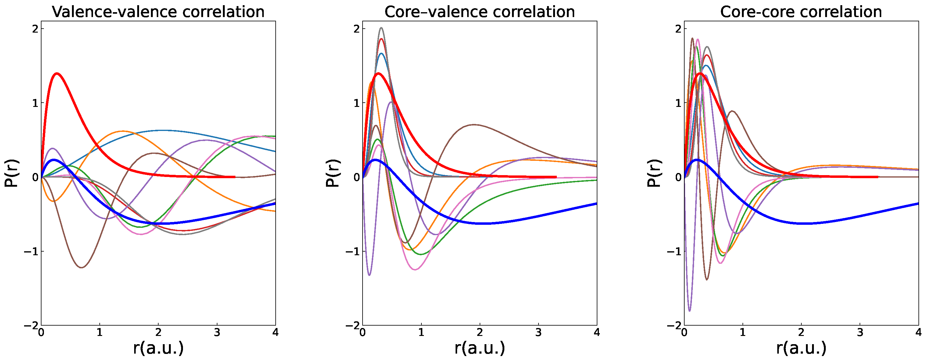
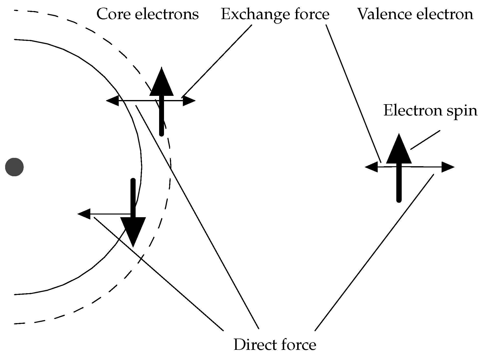
3.2. Polarization Effects

The most important correlation effect for the hyperfine structure is the polarization of the atomic core due to the Coulomb interaction with the valence electrons. Of particular importance is the spin polarization of the closed s shells. If the two s-electrons in the same subshell have different spin densities at the nucleus, a contact interaction is induced in the non-relativistic limit. Since inner s-electrons have high, but canceling, spin densities at the nucleus, a very small imbalance due to the interactions with the outer electrons is sufficient to cause a contribution to the A constant comparable to that of an open valence shell. A schematic illustration is shown in Figure 2. The Coulomb exchange interaction reduces the repulsion between core and valence electrons with the same spin orientation, pulling the core electron towards the valence subshell and causing an imbalance.
For example, consider the 1 s 2 2 s 2 S 1 / 2 and 1 s 2 2 p 2 P 1 / 2 , 3 / 2 o states in 7 Li. In the multiconfiguration method, adhering to the non-relativistic notation, spin polarization (SP) can be described by adding a CSFs of the form Φ ( 1 s 1 s 2 ( 3 S ) 2 s 2 S ) and Φ ( 1 s 1 s 2 ( 3 S ) 2 p 2 P o ) , respectively, to yield
Ψ S P ( 1 s 2 2 s 2 S ) = c 1 Φ ( 1 s 2 2 s 2 S ) + c 2 Φ ( 1 s 1 s 2 ( 3 S ) 2 s 2 S )
and
Ψ S P ( 1 s 2 2 p 2 P o ) = c 1 Φ ( 1 s 2 2 p 2 P o ) + c 2 Φ ( 1 s 1 s 2 ( 3 S ) 2 p 2 P o ) ,
where 1 s 2 is allowed to be non-orthogonal to 1 s and 2 s . For 1 s 2 2 p 2 P o , there is also an orbital polarization (OP), which is due to the interaction of the core with the non-spherical charge distribution of the valence orbital. This interaction distorts the spherical symmetry of the core, leading to additional contributions, in the non-relativistic limit, to the orbital, spin-dipolar, and quadrupole terms. In the multiconfiguration method, orbital polarization can be described by adding CSFs of the forms Φ ( 1 s 3 d 3 ( 3 D ) 2 p 2 P o ) and Φ ( 1 s 3 d 4 ( 1 D ) 2 p 2 P o ) to finally yield
Ψ S P + O P ( 1 s 2 2 p 2 P o ) = c 1 Φ ( 1 s 2 2 p 2 P o ) + c 2 Φ ( 1 s 1 s 2 ( 3 S ) 2 p 2 P o ) + c 3 Φ ( 1 s 3 d 3 ( 3 D ) 2 p 2 P o ) + c 4 Φ ( 1 s 3 d 4 ( 1 D ) 2 p 2 P o ) ,
where 3 d 3 and 3 d 4 are non-orthogonal [17].

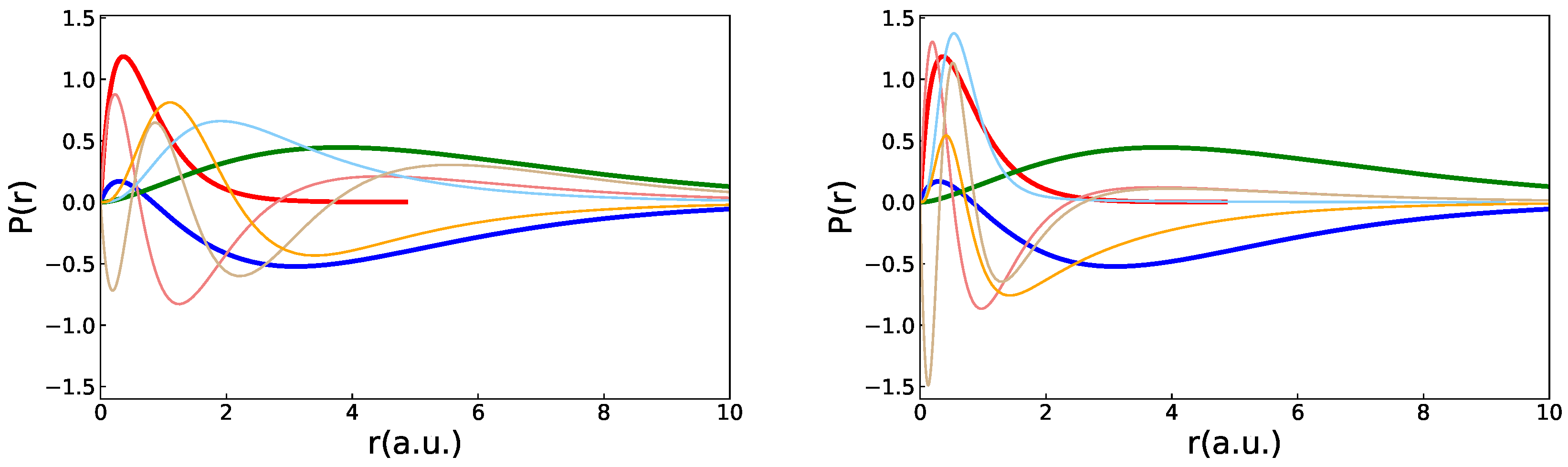
3.3. Localization of the Polarization Orbitals

The efficiency of the above representation relies on the assumption that the correlation orbitals are optimally localized to describe the polarization effects [18]. In relativistic MCDHF calculations, which require the orbitals to be orthonormal in the current version of grasp, such an orbital basis, optimally localized for describing SP and OP, can be obtained as follows:
  • Perform a weighted average Dirac–Fock calculation for 1 s 2 2 s 2 S 1 / 2 and 1 s 2 2 p 2 P 1 / 2 , 3 / 2 o ;
  • Keep 1 s , 2 s , 2 p - , 2 p frozen and perform weighted average MCDHF calculations for 1 s 2 2 s 2 S 1 / 2 and 1 s 2 2 p 2 P 1 / 2 , 3 / 2 o based on the CSF expansions formed by allowing S’s substitution from the reference configuration to a set of s , d - , d orbitals;
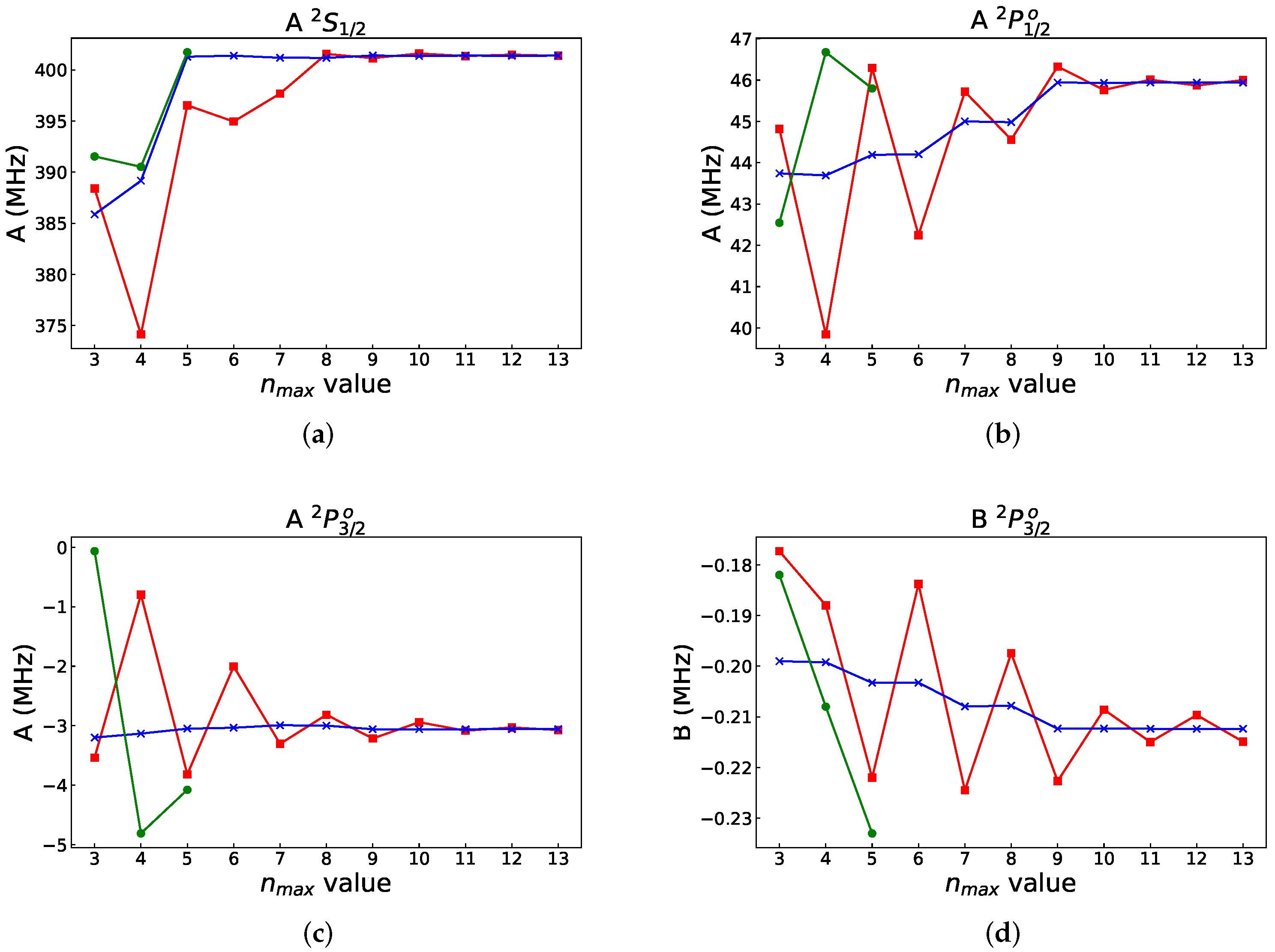
  • Compute the hyperfine interaction constants and monitor the convergence as the set of s , d - , d orbitals is increased;
  • Stop when the hyperfine interaction constants are not changing anymore.
In Table 1, we report the computed hyperfine interaction constants in MHz as functions of the increasing set of s , d - , d orbitals. As can be seen from the table, these small calculations (the calculations based on orbitals with a value of n up to 6 include only 96 CSFs distributed over the three states) already capture the bulk of the correlation effects. Most notable is the hyperfine constant for 1 s 2 2 p 2 P 3 / 2 o , which changes sign when the polarization effects are added.
The radial orbitals resulting from the polarization calculations are shown on the left panel in Figure 3, together with the corresponding spectroscopic 1 s , 2 s , 2 p - , and 2 p orbitals. The polarization orbitals are localized in a region between core electrons and valence electrons to account for the exchange force. For comparison, radial orbitals resulting from an energy-driven calculation, further described in Section 4.1, that include CSFs obtained from SDT substitutions are shown on the right panel in Figure 3. The correlation orbitals from the energy-driven calculation are more contracted, compared with the polarization orbitals, reflecting the fact that the bulk of the correlation energy comes from the interactions within the atomic core. We infer that the orbitals from the energy-driven calculation are unsuited to capture the important polarization effects.

4. Hyperfine Interaction Constants in Different Orbital Bases

4.1. Orbital Basis from Energy-Driven Calculations

We start with weighted average MCDHF calculations for the 1 s 2 2 s 2 S 1 / 2 and 1 s 2 2 p 2 P 1 / 2 , 3 / 2 o states in 7 Li, based on the expansions obtained by allowing single (S), double (D), and triple (T) substitutions from the { 1 s 2 2 s , 1 s 2 2 p } reference configurations to an active set of orbitals. The set is increased layer-by-layer (see [16] §3.5) up to { 13 s , 13 p , 13 d , 13 f , 13 g }. The number of CSFs in the final even and odd state expansions are, respectively, 92 015 and 255 892. These calculations are energy-driven. They include all CSFs that can be generated from the orbital basis, and the orbitals are localized in space by the variational principle, which promotes those correlation effects that maximally lower the weighted energy. In Figure 4, we display, in red squares, the resulting hyperfine interaction constants A and B, in MHz, as functions of the increasing orbital set. The constants were computed using I = 3 / 2 , μ I = 3.256424 μ N , and Q = 0.0406 barn. The behavior for the 1 s 2 2 s 2 S 1 / 2 is irregular, whereas for other states, it is oscillating, making it difficult to establish an accurate final value (cf. Figure 2 in [10]).
The expansions include the CSFs that describe the important polarization effects (single substitutions from the atomic core). However, the orbitals building the CSFs are not spatially localized in the correct region, as seen in Figure 3. The correlation orbitals overlap mainly the 1 s orbital with a tendency for each layer to be either a little more contracted or a little more diffuse each time to lower the weighted energy as much as possible with the resulting oscillations of the hyperfine constants. At the same time, we observe an overall increase in the absolute values of the magnetic dipole hyperfine constants A of the J = 1/2 states, compared with the respective absolute DF values (cf. Table 1). This is consistent with the fact that correlation effects break up the closed atomic core, inducing contributions similar to those from open shells.
It should be noted that the observed oscillations in the hyperfine constants do not result from the layer-by-layer methodology [16] used in this work. A fully variational calculation performed with the MCDFGME code [29,30] for Li-like Be + , Ne 7 + , and Cl 14 + manifested similar oscillatory behavior, although, in the fully variational calculation, the oscillations are slightly more damped than in the layer-by-layer case. The MCDFGME code has also been used to provide fully relaxed, larger-scale calculations for 7 Li, as compared to the calculations from Ref. [31]. The resulting hyperfine constants are displayed as green circles in Figure 4. The wavefunctions include all SDT substitutions to orbitals with n up to 5, i.e., { 5 s , 5 p , 5 d , 5 f , 5 g } , and are fully relaxed. The single substitutions include also those relevant to the Brillouin theorem [32]. This leads to 1463, 1454, and 2478 configurations for the 2 S 1 / 2 , 2 P 1 / 2 o , and 2 P 3 / 2 o states, respectively. It should be pointed out that it is increasingly difficult to obtain convergence in fully variational calculations when increasing the number of orbital layers, and we were unable to go beyond n = 5 . We have included orbitals up to g in both cases and thus should have comparable convergence in the angular correlation contribution. However, full relaxation of all orbitals corresponds to more correlation than in the case whereby the lower orbital layers are kept frozen. Strong oscillations are indeed observed, where most of the differences with the layer-by-layer calculations can be attributed to the fact that the fully relaxed calculations are performed separately for each state in the Optimal Level (OL) approach, whereas the layer-by-layer calculations are performed in the Extended Optimal Level (EOL) approach [33,34].
Oscillatory behavior has also been observed in earlier calculations of hyperfine structures for Sn, Zn, At, Cd, Ra, Au, Hg, Sc, Br, I, Bi, Be + , Fe 6 + , Ti, Y, Sc + , and Y + . Thus, we can conclude that the observed oscillations are inherent to the variational method that prioritizes the energy functional over the targeted atomic property. The latter observation can be understood from the time-independent perturbation theory by looking at the order-by-order expansion of the targeted observable (other than the energy). The terms of this expansion involve matrix elements coupling the zeroeth-order unperturbed states through not only the Hamiltonian but also the relevant (here, hyperfine) operators (cf. Equation (30) in [35]). Many of them do not appear in the energy functional on which the variational principle is applied to derive the MCDHF equations.

4.2. Polarization Orbitals Augmented to the Orbital Basis from Energy-Driven Calculations

Polarization orbitals need to be included in energy-driven layer-by-layer calculations, in order to better describe the correlation effects that are important for the hyperfine constants. However, due to the orthogonality restrictions, separately optimized and optimally localized polarization orbitals can not be directly augmented to the orbital basis from energy-driven layer-by-layer calculations. To overcome the orthogonality constraints, we use the rwfnrelabel program in grasp to relabel (change the principal quantum number that serves as the orbital identifier) the polarization orbitals so that they appear after the orbitals from the energy-driven layer-by-layer calculation. The relabeled polarization orbitals are then, using the rwfnestimate program in grasp, orthogonalized against the orbitals from the energy-driven layer-by-layer calculation and finally augmented. Then, we perform CI calculations with the CSFs obtained by allowing SDT substitutions from the { 1 s 2 2 s , 1 s 2 2 p } reference configurations to orbitals optimized in the energy-driven calculation. To these CSFs, which mainly describe correlation effects that are important for lowering the energy and, to a lesser extent, the effects that are important for the hyperfine structure, we add the CSFs obtained by S substitutions from the atomic core to the augmented, orthogonalized polarization orbitals. For energy-optimized orbital bases with n < 10 , four layers of orthogonalized polarization orbitals were augmented. For energy-optimized orbital bases with n 10 , due to linear dependencies in the orbital basis, only two polarization layers were augmented. The number of CSFs in the final even and odd state expansions are, respectively, 92,541 and 258,432, i.e., only negligibly larger than those from the energy-driven calculation. In Figure 4, we display, in blue crosses, the resulting hyperfine interaction constants A and B in MHz, as functions of the increasing energy-driven orbital set (to which two or four layers of polarization orbitals have been added). Now, the oscillations are almost completely damped out, and the final values of the interaction constants can already be accurately established from a limited, n = 9 , energy-driven orbital set merged with the polarization orbitals. The CPU times of the n = 13 CI calculations are 20m42s in energy-driven calculations and 25m5s for energy-driven orbitals merged with the polarization orbitals’ calculation for the 1 s 2 2 s 2 S 1 / 2 state, using 64 nodes on a cluster with the AMD EPYC 7542 32-Core Processor. The bulk of the CPU time is spent on the calculations for energy-driven orbital sets. The interaction constants, on the other hand, can be accurately established at n = 10 during the calculation of the energy-driven orbital set merged with the polarization orbitals, for which the CPU time of the CI calculation is 6m30s on the 1 s 2 2 s 2 S 1 / 2 state. That means that the efficiency can be improved by using a smaller orbital set compared with energy-driven calculations. The use of separately optimized polarization orbitals merged with energy-driven orbital sets represents a great improvement in both efficiency (the time-consuming parts are the calculations for large energy-driven orbital sets) and accuracy. To provide the final values of the interaction constants, the effects from the neglected orbitals with a higher l, as well as from the Breit interaction, QED, and nuclear recoil, have to be added [31,36,37]. This is, however, outside the scope of the present paper.

5. Summary and Conclusions

Orbitals resulting from MCDHF calculations strongly depend on the employed CSF expansion. Expansions describing, e.g., core–core correlation and other effects aiming at lowering the weighted energy of the targeted states as much as possible may yield an orbital basis that is inadequate for building CSFs that account for correlation effects that are important for other properties. An example is provided by hyperfine interaction constants. These constants are affected by spin and orbital polarizations, described by the CSFs obtained by allowing single substitutions from the atomic core to an orbital basis localized in the region of space between the core electrons and the valence electron(s). This region is energetically unimportant and not well described by the orbitals from energy-driven calculations. The orbitals from energy-driven calculations tend to overlap the orbitals of closed shells; at times they are a little more contracted, and, at other times, they are a little more expanded—a behavior that may lead to oscillations for properties other than the energy. To capture both the energetically important effects as well as the important effects for the hyperfine structure, we propose a procedure in which the polarization orbitals that are optimally localized to describe the polarization effects are relabeled and orthogonalized against orbitals from energy-driven calculations. The procedure is computationally efficient and dramatically improves the convergence properties of the computed hyperfine interaction constants as functions of the increasing orbital set.
The proposed procedure is general and can be applied to compute accurate values of other properties weakly coupled to the energy, as well as energy differences. Applied to the transition parameters from high Rydberg states, it can be used to accurately describe the outer part of the wave function that is important for the length form of the transition operator but energetically unimportant [19]. Applied to energy differences, separate calculations may be performed, targeting core–core, core–valence, and valence–valence electron correlations. The two latter orbital sets are relabeled and orthogonalized against the first one and against each other and then augmented to the first one. In the final CI calculation, the CSFs that account for core–core correlation are built from the core–core orbital set, and the CSFs that account for core–valence correlation are built from the core–core orbital set to which the core–valence orbitals were augmented. Finally, the CSFs that account for valence–valence correlation are built from the full orbital set, including the core–core, core–valence, and valence–valence orbitals. This is similar to the method described in [38], but it uses a merged and orthogonalized orbital basis. It should, in this context, be emphasized that calculations of a specific atomic property require accurate descriptions of effects that are of direct importance for that property, as well as the effects that are important for the total energy, as can be seen from the crossed second-order terms in the perturbative expression for a property (see [35] §7).
Although simple and readily available with the current tools in grasp, rwfnrelabel, and rwfnestimate [22], the present procedure has the drawback that it requires CSFs that are important for the property, or, in the case of energy separations, core–valence, and valence–valence correlation, to be built on merged orbital sets, which implies a certain overhead. An alternate and more general solution circumventing the problems above would be to employ different and mutually non-orthogonal orbital sets and deal with the non-orthogonalities by bi-orthogonal orbital transformations, as in [35,38]. This work is in progress based on the new concept of configuration state function generators (CSFGs) [39].

Author Contributions

Methodology, Y.L., P.J., M.G., G.G., J.B., J.P.M., P.I. and C.C.; software, Y.L., P.J., M.G., G.G., J.B., J.P.M., P.I. and C.C.; validation, Y.L., P.J., M.G., G.G., J.B., J.P.M., P.I. and C.C.; investigation, Y.L., P.J., M.G., G.G., J.B., J.P.M., P.I. and C.C.; writing—original draft, Y.L. and P.J.; writing—review and editing, Y.L., P.J., M.G., G.G., J.B., J.P.M., P.I. and C.C.; visualization, P.J., M.G. and G.G. All authors have read and agreed to the published version of the manuscript.

Funding

This work was supported by the National Natural Science Foundation of China (Grant nos. 12104095 and 12074081). YL acknowledges support from the China Scholarship Council with Grant No. 202006100114. MG acknowledges support from the Belgian FWO & FNRS Excellence of Science Programme (EOSO022818F). This work was also supported by the Fundação para a Ciência e Tecnologia (FCT), Portugal, through contract UIDP/50007/2020 (LIP). P.I. is a member of the Allianz Program of the Helmholtz Association, contract n° EMMI HA-216 “Extremes of Density and Temperature: Cosmic Matter in the Laboratory”. P.I. acknowledges support from the PESSOA Huber Curien Program 2022, Number 47863UE.

Data Availability Statement

Not applicable.

Acknowledgments

The authors wish to thank Charlotte Froese Fischer for the valuable advice and support.

Conflicts of Interest

The authors declare no conflict of interest.

References

  1. Froese Fischer, C.; Gaigalas, G.; Jönsson, P.; Bieroń, J. GRASP2018—A Fortran 95 version of the general relativistic atomic structure package. Comput. Phys. Commun. 2019, 237, 184–187. [Google Scholar] [CrossRef]
  2. Jönsson, P.; Gaigalas, G.; Rynkun, P.; Radžiūtė, L.; Ekman, J.; Gustafsson, S.; Hartman, H.; Wang, K.; Godefroid, M.; Froese Fischer, C.; et al. Multiconfiguration Dirac-Hartree-Fock Calculations with Spectroscopic Accuracy: Applications to Astrophysics. Atoms 2017, 5, 16. [Google Scholar] [CrossRef]
  3. Zhang, C.Y.; Wang, K.; Godefroid, M.; Jönsson, P.; Si, R.; Chen, C.Y. Benchmarking calculations with spectroscopic accuracy of excitation energies and wavelengths in sulfur-like tungsten. Phys. Rev. A 2020, 101, 032509. [Google Scholar] [CrossRef] [Green Version]
  4. Zhang, C.Y.; Wang, K.; Si, R.; Godefroid, M.; Jönsson, P.; Xiao, J.; Gu, M.F.; Chen, C.Y. Benchmarking calculations with spectroscopic accuracy of level energies and wavelengths in W LVII–W LXII tungsten ions. J. Quant. Spectrosc. Radiat. Transf. 2021, 269, 107650. [Google Scholar] [CrossRef]
  5. Zhang, C.Y.; Li, J.Q.; Wang, K.; Si, R.; Godefroid, M.; Jönsson, P.; Xiao, J.; Gu, M.F.; Chen, C.Y. Benchmarking calculations of wavelengths and transition rates with spectroscopic accuracy for W xlviii through W lvi tungsten ions. Phys. Rev. A 2022, 105, 022817. [Google Scholar] [CrossRef]
  6. Andersson, M.; Grumer, J.; Ryde, N.; Blackwell-Whitehead, R.; Hutton, R.; Zou, Y.; Jönsson, P.; Brage, T. Hyperfine-dependent gf values of Mn I lines in the 1.49–180 μm H Band. Astrophys. J. Suppl. 2015, 216, 21. [Google Scholar] [CrossRef] [Green Version]
  7. Si, R.; Brage, T.; Li, W.; Grumer, J.; Li, M.; Hutton, R. A First Spectroscopic Measurement of the Magnetic-field Strength for an Active Region of the Solar Corona. Astrophys. J. Lett. 2020, 898, L34. [Google Scholar] [CrossRef]
  8. Filippin, L.; Bieroń, J.; Gaigalas, G.; Godefroid, M.; Jönsson, P. Multiconfiguration calculations of electronic isotope-shift factors in Zn I. Phys. Rev. A 2017, 96, 042502. [Google Scholar] [CrossRef] [Green Version]
  9. Ekman, J.; Jönsson, P.; Godefroid, M.; Nazé, C.; Gaigalas, G.; Bieroń, J. ris4: A program for relativistic isotope shift calculations. Comput. Phys. Commun. 2019, 235, 433–446. [Google Scholar] [CrossRef]
  10. Bieroń, J.; Froese Fischer, C.; Fritzsche, S.; Gaigalas, G.; Grant, I.P.; Indelicato, P.; Jönsson, P.; Pyykkö, P. Ab initio MCDHF calculations of electron-nucleus interactions. Phys. Scr. 2015, 90, 054011. [Google Scholar] [CrossRef]
  11. Papoulia, A.; Schiffmann, S.; Bieroń, J.; Gaigalas, G.; Godefroid, M.; Harman, Z.; Jönsson, P.; Oreshkina, N.S.; Pyykkö, P.; Tupitsyn, I.I. Ab initio electronic factors of the A and B hyperfine structure constants for the 5s25p6s 1,3P1o states in Sn I. Phys. Rev. A 2021, 103, 022815. [Google Scholar] [CrossRef]
  12. Li, J.; Gaigalas, G.; Bieroń, J.; Ekman, J.; Jönsson, P.; Godefroid, M.; Froese Fischer, C. Re-Evaluation of the Nuclear Magnetic Octupole Moment of 209Bi. Atoms 2022, 10, 132. [Google Scholar] [CrossRef]
  13. Barzakh, A.; Andreyev, A.N.; Raison, C.; Cubiss, J.G.; Van Duppen, P.; Péru, S.; Hilaire, S.; Goriely, S.; Andel, B.; Antalic, S.; et al. Large shape staggering in neutron-deficient Bi isotopes. Phys. Rev. Lett. 2021, 127, 192501. [Google Scholar] [CrossRef] [PubMed]
  14. Wraith, C.; Yang, X.; Xie, L.; Babcock, C.; Bieroń, J.; Billowes, J.; Bissell, M.; Blaum, K.; Cheal, B.; Filippin, L.; et al. Evolution of nuclear structure in neutron-rich odd-Zn isotopes and isomers. Phys. Lett. B 2017, 771, 385–391. [Google Scholar] [CrossRef]
  15. Barzakh, A.; Cubiss, J.; Andreyev, A.; Seliverstov, M.; Andel, B.; Antalic, S.; Ascher, P.; Atanasov, D.; Beck, D.; Bieroń, J.; et al. Inverse odd-even staggering in nuclear charge radii and possible octupole collectivity in 217,218,219At revealed by in-source laser spectroscopy. Phys. Rev. C 2019, 99, 054317. [Google Scholar] [CrossRef] [Green Version]
  16. Jönsson, P.; Godefroid, M.; Gaigalas, G.; Ekman, J.; Grumer, J.; Li, W.; Li, J.; Brage, T.; Grant, I.P.; Bieroń, J.; et al. An introduction to relativistic theory as implemented in GRASP. Atoms 2022, in press. [Google Scholar]
  17. Froese Fischer, C.; Brage, T.; Jönsson, P. Computational Atomic Structure; Institute of Physics Publishing (IoP): Bristol, UK, 1997. [Google Scholar]
  18. Godefroid, M.R.; Van Meulebeke, G.; Jönsson, P.; Froese Fischer, C. Large-scale MCHF calculations of hyperfine structures in nitrogen and oxygen. Z. Phys. D—Atoms Mol. Clust. 1997, 42, 193–201. [Google Scholar] [CrossRef]
  19. Papoulia, A.; Ekman, J.; Gaigalas, G.; Godefroid, M.; Gustafsson, S.; Hartman, H.; Li, W.; Radžiūtė, L.; Rynkun, P.; Schiffmann, S.; et al. Coulomb (Velocity) Gauge Recommended in Multiconfiguration Calculations of Transition Data Involving Rydberg Series. Atoms 2019, 7, 106. [Google Scholar] [CrossRef] [Green Version]
  20. Grant, I.P. Relativistic Quantum Theory of Atoms and Molecules: Theory and Computation; Springer Science and Business Media, LLC: New York, NY, USA, 2007. [Google Scholar]
  21. Froese Fischer, C.; Godefroid, M.; Brage, T.; Jönsson, P.; Gaigalas, G. Advanced multiconfiguration methods for complex atoms: I. Energies and wave functions. J. Phys. B At. Mol. Opt. Phys. 2016, 49, 182004. [Google Scholar] [CrossRef] [Green Version]
  22. Jönsson, P.; Godefroid, M.; Gaigalas, G.; Ekman, J.; Grumer, J.; Li, W.; Li, J.; Brage, T.; Grant, I.P.; Bieroń, J.; et al. GRASP Manual for Users. Atoms 2022, in press. [Google Scholar]
  23. Godefroid, M.R.; Jönsson, P.; Froese Fischer, C. Atomic structure variational calculations in spectroscopy. Phys. Scr. 1998, 1998, 33. [Google Scholar] [CrossRef] [Green Version]
  24. Schwartz, C. Theory of hyperfine structure. Phys. Rev. 1955, 97, 380. [Google Scholar] [CrossRef]
  25. Lindgren, I.; Rosén, A. Relativistic self-consistent-field calculations with application to atomic hyperfine interaction. Case Stud. At. Phys. 1974, 3, 93–196. [Google Scholar]
  26. Lindgren, I. Effective operators in the atomic hyperfine interaction. Rep. Prog. Phys. 1984, 47, 345. [Google Scholar] [CrossRef]
  27. Beckmann, A.; Böklen, K.; Elke, D. Precision measurements of the nuclear magnetic dipole moments of 6Li, 7Li, 23Na, 39K and 41K. Z. Phys. 1974, 270, 173–186. [Google Scholar] [CrossRef]
  28. Orth, H.; Ackermann, H.; Otten, E. Fine and hyperfine structure of the 2 2P term of 7Li; determination of the nuclear quadrupole moment. Z. Phys. A Atoms Nucl. 1975, 273, 221–232. [Google Scholar] [CrossRef]
  29. Desclaux, J. A multiconfiguration relativistic DIRAC-FOCK program. Comput. Phys. Commun. 1975, 9, 31–45. [Google Scholar] [CrossRef]
  30. Indelicato, P. Projection operators in multiconfiguration Dirac-Fock calculations: Application to the ground state of heliumlike ions. Phys. Rev. A 1995, 51, 1132–1145. [Google Scholar] [CrossRef]
  31. Boucard, S.; Indelicato, P. Relativistic Many-Body and Qed Effects on the Hyperfine Structure of Lithium-Like Ions. Eur. Phys. J. A 2000, 8, 59–73. [Google Scholar] [CrossRef]
  32. Indelicato, P.; Lindroth, E.; Desclaux, J. Nonrelativistic Limit of Dirac-Fock Codes: The Role of Brillouin Configurations. Phys. Rev. Lett. 2005, 94, 013002. [Google Scholar] [CrossRef] [Green Version]
  33. Grant, I.P.; McKenzie, B.J.; Norrington, P.H.; Mayers, D.F.; Pyper, N.C. An atomic multiconfigurational Dirac-Fock package. Comput. Phys. Commun. 1980, 21, 207–231. [Google Scholar] [CrossRef]
  34. Dyall, K.G.; Grant, I.P.; Johnson, C.T.; Parpia, F.A.; Plummer, E.P. GRASP: A general-purpose relativistic atomic structure program. Comput. Phys. Commun. 1989, 55, 425–456. [Google Scholar] [CrossRef]
  35. Verdebout, S.; Rynkun, P.; Jönsson, P.; Gaigalas, G.; Froese Fischer, C.; Godefroid, M. A partitioned correlation function interaction approach for describing electron correlation in atoms. J. Phys. B At. Mol. Opt. Phys. 2013, 46, 085003. [Google Scholar] [CrossRef]
  36. Bieroń, J.; Jönsson, P.; Froese Fischer, C. Large-scale multiconfiguration Dirac-Fock calculations of the hyperfine-structure constants of the 2s 2S1/2, 2p 2P1/2, and 2p 2P3/2 states of lithium. Phys. Rev. A 1996, 53, 2181–2188. [Google Scholar] [CrossRef] [PubMed]
  37. Puchalski, M.; Pachucki, K. Ground State Hyperfine Splitting in 6,7Li Atoms and the Nuclear Structure. Phys. Rev. Lett. 2013, 111, 243001. [Google Scholar] [CrossRef] [PubMed] [Green Version]
  38. Froese Fischer, C.; Verdebout, S.; Godefroid, M.; Rynkun, P.; Jönsson, P.; Gaigalas, G. Doublet-quartet energy separation in boron: A partitioned-correlation-function-interaction method. Phys. Rev. A 2013, 88, 062506. [Google Scholar] [CrossRef] [Green Version]
  39. Li, Y.T.; Wang, K.; Si, R.; Godefroid, M.; Gaigalas, G.; Chen, C.Y.; Jönsson, P. Reducing the computational load—Atomic multiconfiguration calculations based on configuration state function generators. Comput. Phys. Commun. 2023, 283, 108562. [Google Scholar] [CrossRef]
Figure 1. Contraction of the correlation orbitals when going from valence–valence through core–valence to core–core correlation MCDHF calculations of 1 s 2 2 s 2 1 S 0 state of Be. The two thick lines correspond to the 1 s (red, no node) and 2 s (blue, one node) orbitals. Other lines represent the radial distributions of the correlation orbitals with n up to 4.
Atoms 11 00004 g001
Figure 2. Spin polarization of a closed subshell in the core due to the Coulomb interaction with an open valence subshell (cf. Figure 7 in Lindgren’s paper [26]).
Atoms 11 00004 g002
Figure 3. Left: orbitals from a calculation including CSFs describing polarization effects. Right: orbitals from an energy-driven calculation, including CSFs obtained from SDT substitutions. The three thick lines correspond to the spectroscopic 1 s (red, no node), 2 s (blue, one node), and 2 p (green, no node) orbitals.
Atoms 11 00004 g003
Figure 4. Convergence of hyperfine constants (a) A ( 1 s 2 2 s 2 S 1 / 2 ) , (b) A ( 1 s 2 2 p 2 P 1 / 2 o ) , (c) A ( 1 s 2 2 p 2 P 3 / 2 o ) and (d) B ( 1 s 2 2 p 2 P 3 / 2 o ) of 7 Li (all in MHz) from the energy-driven layer-by-layer calculations (red squares), from the energy-driven fully variational calculations using the MCDFGME code (green circles), and from calculations with merged polarization orbitals (blue crosses). The difference in the convergence patterns between the energy-driven layer-by-layer GRASP calculations and the energy-driven fully variational calculations with MCDFGME is probably due to the fact that the former were performed by simultaneously optimizing the three states in the extended optimal level (EOL) approach, whereas in the latter case, each state was separately optimized (OL).
Atoms 11 00004 g004
Table 1. Hyperfine interaction constants (in MHz) for the 1 s 2 2 s 2 S 1 / 2 and 1 s 2 2 p 2 P 1 / 2 , 3 / 2 o states in 7 Li from weighted average DF calculations and weighted average MCDHF calculations including spin and orbital polarization effects with four layers of s , d - , d orbitals, i.e., orbitals set up to { 6 s , 6 d - , 6 d } . The nuclear parameters for 7 Li are I = 3 / 2 , μ I = 3.256424 μ N , and Q = 0.0406 barn.
A ( 2 S 1 / 2 ) A ( 2 P 1 / 2 o ) A ( 2 P 3 / 2 o ) B ( 2 P 3 / 2 o )
DF290.24932.356−6.469 0.2235
{ 3 s , 3 d - , 3 d } 374.04744.741 4.910 0.2238
{ 4 s , 4 d - , 4 d } 380.69242.461 2.619 0.1968
{ 5 s , 5 d - , 5 d } 380.34142.610 2.766 0.1968
{ 6 s , 6 d - , 6 d } 380.34242.611 2.766 0.1968
Exp.401.752043 a 45.914(25) b −3.055(14) b
a Ref. [27], b Ref. [28].
Disclaimer/Publisher’s Note: The statements, opinions and data contained in all publications are solely those of the individual author(s) and contributor(s) and not of MDPI and/or the editor(s). MDPI and/or the editor(s) disclaim responsibility for any injury to people or property resulting from any ideas, methods, instructions or products referred to in the content.

