Real World Vehicle Emission Factors for Black Carbon Derived from Longterm In-Situ Measurements and Inverse Modelling

Abstract

Black carbon (BC) is one of the most harmful substances within traffic emissions, contributing considerably to urban pollution. Nevertheless, it is not explicitly regulated and the official laboratory derived emission factors are barely consistent with real world emissions. However, realistic emission factors (EFs) are crucial for emission, exposure, and climate modelling. A unique dataset of 10 years (2009–2018) of roadside and background measurements of equivalent black carbon (eBC) concentration made it possible to estimate real world traffic EFs and observe their change over time. The pollutant dispersion was modelled using the Operational Street Pollution Model (OSPM). The EFs for eBC are derived for this specific measurement site in a narrow but densely trafficked street canyon in Leipzig, Germany. The local conditions and fleet composition can be considered as typical for an inner-city traffic scenario in a Western European city. The fleet is composed of 22% diesel and 77% petrol cars in the passenger car segment, with an unknown proportion of direct injection engines. For the mixed fleet the eBC EF was found to be 48 mg km${}^{-1}$ in the long-term average. Accelerated by the introduction of a low emission zone, the EFs decreased over the available time period from around 70 mg km${}^{-1}$ to 30–40 mg km${}^{-1}$. Segregation into light (<3.5 t) and heavy (>3.5 t) vehicles resulted in slightly lower estimates for the light vehicles than for the mixed fleet, and one order of magnitude higher values for the heavy vehicles. The found values are considerably higher than comparable emission standards for particulate matter and even the calculations of the Handbook Emission Factors for Road Transport (HBEFA), which is often used as emission model input.

1. Introduction

On-road traffic is one of the most important contributors to pollution by particulate matter (PM) in urban environments [1], evidently affecting not only human health and lifetime adversely [2], but also playing a major role in climate discussions [3]. However, the uncertainties connected to the numbers and processes are large, especially for black carbon (BC). Various studies have shown BC to be the most harmful component in particulate emissions towards human health, introducing heavy metals and PAHs deep into the cardiovascular system (see [4,5], and references therein).

Realistic emission factors are required for various purposes like modelling climate impact on a global scale, creating emission inventories on a regional scale, down to modelling citizen exposure on a municipal level. Models like these are also used as a tool to estimate the need for reduction measures and to evaluate their potential on pollution mitigation. For this, they need to be fed with realistic time resolved emission factors. A first indication could be the official manufacturers statements on vehicle emissions.

In Germany, new vehicle types have to receive a type approval, for which the manufacturers have to ensure that the vehicles—among other regulations—meet the emission standards established by the European Union [6]. The regulated parameters include Hydrocarbons (HC), CO and NO${}_x$. Black carbon is only indirectly regulated through the mass of particulate matter (PM, <4.5 mg km${}^{-1}$ from 2011/Euro5a) and particle number (PN, <6$·{10}^{11}$ km${}^{-1}$ from 2013/Euro5b) [6]. The values that must compare to the emission standards are derived through measurements conducted on chassis dynamometers. Since on-road emission studies were frequently off the limits (especially NO${}_x$, [7]), in 2017 the EU established additional test procedures for so called real driving emissions (RDE). The Handbook Emission Factors for Road Transport (HBEFA) [8] is an attempt to derive more realistic EFs. For this database, test bench values, also beyond regulatory test criteria, as well as RDE measurements (from version 3.3 on) of individual vehicles are adapted to on road fleet conditions via the emission simulation model PHEM (Passenger Car and Heavy Duty Emission Model) [9]. It yields average EFs for the engine maps of the different vehicle types and emission levels. Then standardised driving cycles for different traffic situations (e.g., including information on speed limits, road types and road congestion) are applied. Moreover, the EFs are weighted for shares in new registrations. In addition to the regulated pollutants, emission factors for BC were included in Version 4.1. (2019).

Diesel vehicles have long been associated with higher soot emissions and have therefore been subject to increasingly strict limits. Diesel particulate filters (DPFs) became necessary to meet these limits. Nevertheless, various circumstances can lead to higher emissions on the street. When the DPF is regenerated by burning the collected soot, the emission is significantly higher than in normal operation [10]. If a diesel vehicle is used too seldom for long distance drives, this process could be initiated even within the already more polluted cities [10]. Another problem lies in the sensitivity of the opacimeters, used for the regular inspections, which is currently not sufficient to detect removed, manipulated or malfunctioning (e.g., due to microfissures) DPFs [11]. Dutch studies found 5 to 7% of the DPFs removed or defect [11]. If such defects remain undetected, it can be assumed that the vehicles emit up to several times more. However, the emissions not only originate from diesel vehicles. Several studies showed, that even though consuming less fuel while emitting less CO${}_2$ and other gas-phase pollutants, gasoline direct injection (GDI) engines emit a significant amount of particles [12]. Saliba et al. [13] found GDIs to emit up to twice the amount of PM compared to conventional port fuel injection (PFI) engines. They are nearly equalling the emission level of diesel engines [14]. Additionally, also PFI vehicles can emit considerable amounts of particles [12] while the limits for particulates only apply to GDI engines [6]. Furthermore, the real world fleet-even though evolving towards higher emission standards—includes a certain amount of aged vehicles which can disproportionally contribute to overall emissions [15]. Moreover, peoples driving habits usually do not comply with standard protocols.

To obtain a realistic fleet averaged EF of BC, it needs different approaches than test stand EFs of individual brand new cars. Even RDE might only be part of a solution since it does not cover all realistic driving scenarios [16]. Moreover, as required for the type approval tests, it only covers PN, but not PM [17]. In the end, real world fleet emission factors are supposed to give us an estimate of how much an actual vehicle emits on the streets in everyday life per kilometer driven. Like this, they can be used for example to estimate exposure levels, evaluate reduction measures or to assess the climatic relevance of an emitted substance.

There are various studies using different methods to determine such EFs. An overview of possible approaches can be found in Franco et al. [18]. Comparable to the industrial RDE-tests, on-road-measurements are used to determine emissions while driving in regular traffic. Portable emission measurement systems (PEMS) are mounted onto the vehicle, allowing parallel logging of emissions and driving parameters. Due to the more realistic—but changing—conditions though, the measurements of the vehicles are not as comparable any more. Furthermore, this method needs a lot of effort to produce a statistically significant dataset. Apart from that, these measurements can only reflect the fleet as a mixture of old and new vehicles in different stages of repair and maintenance to a limited extent. Similar approaches to probe single vehicles coming closer to represent the whole fleet, include car chasing methods or remote sensing of car plumes. However, only a sample of single vehicles can be measured. A completely different approach, which probes the vehicle fleet on a street as a whole, is the use of inverse modelling. Using a closed volume, tunnel studies can provide real world emission factors by correlating the pollutant flux to the fleet passing the tunnel. Moreover, an open volume such as a street canyon can be used for an inverse approach with an appropriate dispersion model. This method was used to analyse the dataset presented here.

Apart from the absolute amount of emissions, another important aspect is their development over time. Typically though, real emission studies are based on short term observations or intensive campaigns. In line with the increasingly strict regulation of emissions and the ongoing technical evolution, the collective fleet emissions could be expected to decrease. Additionally, the uptake of environmental measures such as the installation of low emission zones, accelerates the renewal of the fleet. On the other hand, the number of registrations of diesel-powered vehicles is increasing steadily. And the registration numbers of gasoline GDI powered cars are increasing as well.

With our study, we aim to estimate realistic emission factors for equivalent black carbon (eBC, a terminology suggested by Petzold 2013 [19] for optically measured BC), representing the mixed fleet in an urban environment and to observe their change over time. To achieve this goal, we analysed a set of 10 years of continuous measurements using an inverse modelling approach.

2. Methods

2.1. The Method of Inverse Modelling

To retrieve traffic EFs for eBC, the already established method of inverse modelling [20] combined with the so called Lenschow approach [21] was chosen. The major sources for BC within cities are traffic and biomass burning [3], mixed with long range transport sources. To separate the different sources, a traffic increment $C_{tr}(\mathsf{\mu }\mathrm{g}{\mathrm{m}}^{-3})$ was calculated by subtracting a measured reference value for the urban background $C_{bg}$ from the roadside station measurement $C_{rs}$.

$$C_{tr}=C_{rs}-C_{bg}$$

(1)

with this approach, also the influence of any large scale meteorology (e.g., inversion weather conditions with high pollutant concentration) on the estimated emission factor can be minimized. It is assumed that the increment only represents the eBC emitted by the passing traffic [21]. To be statistically robust, the difference between roadside station and background should be significant though. Otherwise, small uncertainties of the measurements might lead to biased or even negative values of the increment and subsequently emission factors. The relation of the total emission $Q\left(\mathrm{mg}{\mathrm{km}}^{-1}{\mathrm{s}}^{-1}\right)$ at the source and the traffic concentration increment $C_{tr}$ at the receptor is described by the so called dilution factor $F\left(\mathrm{s}{\mathrm{m}}^{-2}\right)$. Including the traffic density $N_V\left({\mathrm{s}}^{-1}\right)$, the emission factor $q\left(\mathrm{mg}{\mathrm{km}}^{-1}\right)$ for the average single vehicle can be estimated with

$$q=\frac{C_{tr}}{F·N_V}.$$

(2)

For a single measurement the uncertainty of the retrieved EF is very high due to the fact that several parameters, each with its own uncertainty, go into the calculation. For larger datasets, the emission factor can be more robustly derived as the slope from a linear regression of the traffic eBC increment against the dilution factor times the traffic density. Assuming that the different source types i sum up, the equation

$$Q=\sum _{i=1}^n{q}_i·N_i$$

(3)

can be used for a multivariate linear regression to derive the emission factors for different groups of the fleet. Required for this approach are the respective traffic density numbers for these groups. In our case, we can distinguish between light vehicles (LV) below 3.5 t and heavy vehicles (HV) above 3.5 t. With Equations (2) and (3) a bivariate linear regression can be performed as

$$C_{tr}=q_{LV}·F·N_{LV}+q_{HV}·F·N_{HV}.$$

(4)

A strong limitation for this split approach though, is the need for relative changes in the fleet composition. The more pronounced these changes are (e.g., almost no trucks on Sundays, a very high fraction on Mondays) the more reliable the fitting parameters are. Besides the local topography, especially wind influences the measured value at the roadside station. Depending on speed and direction of the wind, the emitted pollutants are more or less diluted. In case of a simple topography, like a street canyon, the flow regime can be modelled with low-effort and user friendly models like Operational Street Pollution Model (OSPM) [22]. For the special case of a street canyon geometry-commonly defined as a narrow street with buildings on either side-significant concentration differences can develop if the wind blows perpendicular to the street axis. With the height of the buildings and the width of the street being approximately the same, a vortex forms making the wind direction at street level the opposite to the roof level wind. Like that, on the leeward side of the street the traffic emissions accumulate, whereas at the windward side fresh air from above the roofs is entrained and the concentrations are much lower. Figure 1 (left) illustrates this effect for a perpendicular wind direction at roof level.

2.2. The OSPM

Originally designed as a forward model, the OSPM (Operational Street Pollution Model) [22] can be used to describe the relation between emission source and receptor, yielding the dilution factor F. It was developed by the National Environmental Research Institute of Denmark, Department of Atmospheric Environment, Aarhus University. The semi-empirical dispersion model predicts the concentration of traffic emissions at both walls of a street canyon for different pollutants, using a plume model for the direct emissions and a box model for the recirculated part. This value only depends on the input parameters wind speed and direction as well as the vehicle density and their individual emissions. For very low wind speeds the OSPM also considers turbulence induced by the vehicles. The dilution factor F can be derived through dividing the modelled concentration by the total emission. It then only depends on the canyon geometry and the wind and turbulence conditions and may be applied to all inert pollutants emitted by the traffic.

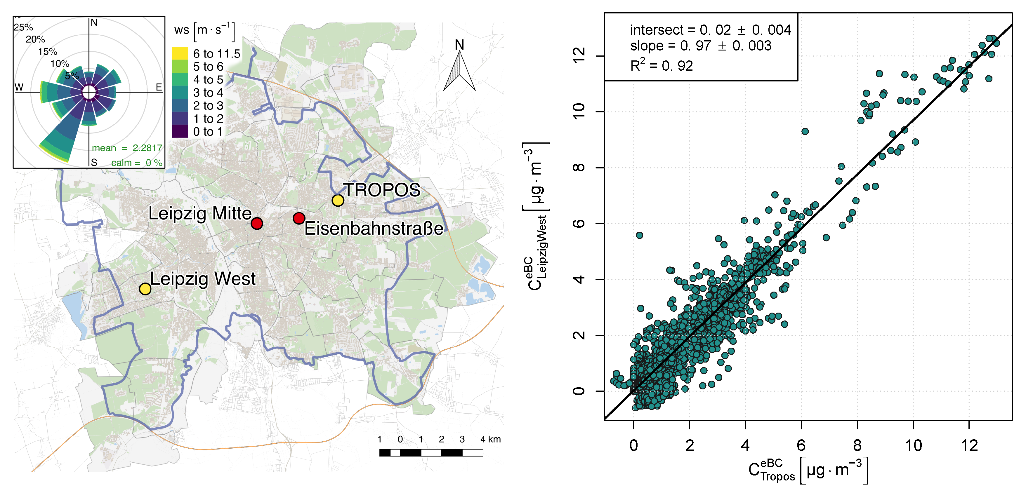
2.3. Measurement Sites and Instruments

For the calculation of the emission factors, sets of roadside stations and rural background stations [21] are required. Figure 2 (left) shows the location of the available stations within the city of Leipzig. In this work we will focus on the station Eisenbahnstraße (EIBA) representing a roadside station. The measurements on the grounds of the Institute for Tropospheric Research (TROPOS) and in Leipzig West (LEW) represent the urban background. Although the two background stations are located in different parts of the city they are well correlated (Figure 2, right; $\mathrm{slope}=0.97,$ R${}^2=0.92$) and are therefore assumed to appropriately represent the urban background. For better statistics, the background value was calculated as the mean of the two stations, when data from both was available. Otherwise the remaining station value was used. Subtracting the background value from the value measured at the roadside station, yields the traffic induced concentration increment. From source apportionment studies, it is known that this assumption is valid for the used stations: Van Pinxteren et al. [23] found that the contribution by coal and biomass burning to the particle size range of 0.05–0.14 $\mathsf{\mu }$m is very similar for EIBA and TROPOS, even in winter, whereas the values for the exhaust traffic category are significantly higher for the roadside EIBA station. Apparently, the contribution of heating blends in with the background and we can use the increment for further calculations of the traffic emission factor.

The station EIBA (Figure 1, right) is situated inside a classical street canyon where the building height of about 20 m corresponds to the width of the street. A distinct feature of the site is the junction with the Herman-Liebmann-Straße, where the traffic is regulated by traffic lights. The instruments are placed inside a first floor apartment on the northern side of the street which has a 94${}^{\circ }$ east-west-orientation. With one lane in both directions each, about 10,000 vehicles pass the station on a weekday and almost 6000 on Sundays. The PM${}_{10}$ inlet for the aerosol measurements has a height of about 7 m above ground. A Multi Angle Absorption Photometer (MAAP) by Thermo Scientifc is used to obtain the mass of black carbon. A detailed description of the filter based instrument is given by Petzold and Schönlinner [24]. They estimated the uncertainty of the MAAP to be 12%. Müller et al. [25] found a unit to unit variability of less than 5%. The instruments were subjected to regular maintenance. Functional checks were carried out approximately every two weeks. Regularly, also flow rate and zero checks are applied. If no irregularities occur before, larger intercomparison workshops are conducted on an annual to biennial basis. As implemented within the MAAP software the relation of

$$\sigma {}_{abs}=C_{eBC}·\alpha {}_{eBC}$$

(5)

is used to convert the particle light absorption coefficient ${\sigma }_{abs}$ (${\mathrm{Mm}}^{-1}$) and the concentration of black carbon $C_{eBC}$ ($\mathrm{g}{\mathrm{m}}^{-3}$) with a mass absorption coefficient (MAC) of $\alpha {}_{eBC}=6.6{\mathrm{m}}^2$ g${}^{-1}$. Furthermore, a correction factor of 1.05 is applied, to account for the true MAAP wavelength of 637 nm (instead of 670 nm, as stated by the manufacturer) [25]. Since it is not determined gravimetrically, but optically via a conversion using a fixed MAC, we use the terminology equivalent black carbon (eBC) as suggested by Petzold 2013 [19].

Wind speed and direction were measured about 4 m above roof top level using a sonic anemometer (model USA-1, Metek GmbH, Elmshorn, Germany). Good agreement with other stations around the city was found within expected variations. The manufacturer gives a 0.1 m s${}^{-1}$ or 2% accuracy for wind speed and 2${}^{\circ }$ at 5 m s${}^{-1}$ for wind direction.

The traffic density could not be recorded continuously throughout the measurements. An automated count from March to November 2005, based on a video detection system (Autoscope Rackvision, Image Sensing Systems (ISS), St. Paul, MN, USA), is available for the station EIBA. The light (<3.5 t) and heavy (>3.5 t) vehicles were distinguished via the length of the vehicles detected. With this method, it is not possible to differentiate between passenger cars and light commercial vehicles. Therefore, we stick to the terms light and heavy vehicles (LV and HV), in contrast to other studies that use LDV and HDV. For a second period, two weeks in September 2015, manually counted data is available. Although the statistics is worse, the absolute values are about the same as for the automated counting in 2005 within appropriate uncertainties. Evidently, there had not been a significant change in traffic volume. The weekly traffic profile was therefore adapted for the whole time without further adjustment. An attempt to correct the data for a possible long term trend was discarded (see Appendix A for details). Manual evaluation of the countings yielded an accuracy of ± 3% for the light vehicle class and ± 10% for the heavy vehicles during daylight hours. Moving light cones and shadows, though, caused problems in the dark, leading to significant overestimation of the traffic density during the night. For this reason only the classification during the day was used to calculate the emission factors. It was not possible to distinguish between diesel and petrol engines with this detection method. Statistics for Saxony by the Kraftfahrt-Bundesamt (KBA [26]) though give a share of about 22% diesel and 77% petrol cars in the passenger segment, averaged over the years 2009–2018. Within this time the share of diesel was rising steadily from 17.4% (1 January 2009) to 26.8% (1 January 2019).

3. Results

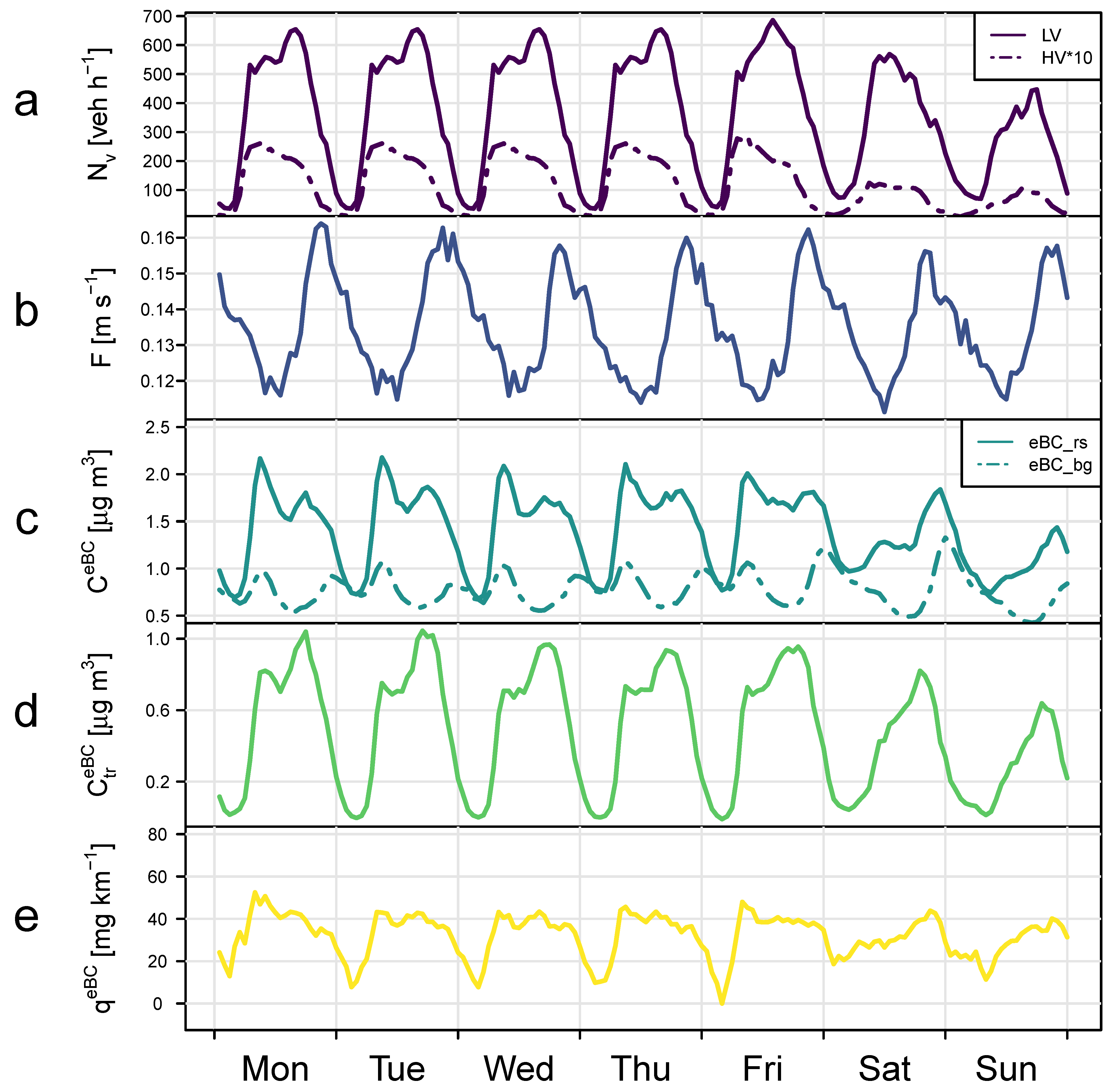
3.1. Dataset Overview

Equivalent black carbon was measured at a roadside and two background stations. Our analysis is based on 1-hour-median values. The overall median is 0.75 $\mathsf{\mu }$g m${}^{-3}$ for the background and 1.36 $\mathsf{\mu }$g m${}^{-3}$ for the roadside station, respectively. This gives an average ratio background to roadside of 0.66. Splitting into the days of the week yields 0.64, 0.69 and 0.73 for weekdays, Saturdays and Sundays, respectively. With the formerly described method it is possible to simulate dilution factors for the period 2009–2018. They cover a plausible range from 0 to 0.4 s m${}^{-2}$ for 1 h mean values.

Figure 3 illustrates the traffic profile and the median weekly patterns of the relevant parameters. In panel (a) the traffic counts per hour are shown for light vehicles as solid line and heavy vehicles as dotted line (multiplied by 10 for better visibility). For Monday through Thursday the measured traffic profile showed only marginal variation and was therefore assumed constant for better statistics. On Friday though, the decrease in the afternoon starts a bit earlier. On Saturday and Sunday the amount of traffic is reduced and the profile, not showing the distinct bimodal pattern any more, is slightly shifted to later times. The daily amount of vehicles sums up to about 10,000 vehicles during working days, just above 8000 on Saturdays and almost 6000 on Sundays. The relative amount of heavy vehicles varies between 1 and 6%.

The dilution factor F (b) depends mainly on the wind speed and direction and therefore shows its minimum (strongest dilution) around noon and the early afternoon. Accordingly, the day-of-the-week variation is random.

Panel (c) shows the concentration of black carbon at the background (dotted) and the roadside (solid) measurement stations, respectively. The roadside station shows a strong similarity with the traffic count pattern, apart from a local minimum at noon, coinciding with the growth of the boundary layer and mixing height. The background concentration has a rather strong minimum that outweighs the traffic influence by far. The later maximum is not as pronounced as in the traffic density. A reason for that is also the higher boundary layer at this time of day, where the pollutants can distribute within a larger volume. Especially in the street canyon also the higher wind speed can lead to a stronger dilution and therefore lower concentrations in the second half of the day (see panel (b)). In the weekly pattern, the roadside concentration reaches up to 2.2 $\mathsf{\mu }$g m${}^{-3}$ during the morning peak and drops down to the background value which is typically below 1 $\mathsf{\mu }$g m${}^{-3}$ during the night.

The increment of roadside and background measurement and therefore the contribution of the traffic is shown in panel (d). It peaks around 1 $\mathsf{\mu }$g m${}^{-3}$ and decreases to almost zero during the night. (Figure 6 shows the same data, broken down by year.)

Panel (e) in Figure 3 shows the estimated eBC EF and the problems that arise during the night and early morning hours. Since the estimated EF of the single vehicle is not influenced by any external factors like the traffic density, the wind, and the measured concentrations, it should not have any significant pattern. Because of the division of small numbers (eBC concentration at night) by other small numbers with high uncertainty (traffic density at night), and sudden changes as is the case in the early morning, large uncertainties arise in the calculated EF. For that reason, the following analyses will only consider the EF during the daytime hours from 7 am to 8 pm. On the weekend days the EF shows a significant decrease. A reason for that could be the circumstance, that it is calculated from the total vehicle count, but the share of heavy vehicles-and therefore strong contributors-is lower on those days.

Another limitation for the chosen Lenschow approach are certain conditions, when the background and roadside concentrations are very similar. This happens for example during the night, when the traffic contribution is lowest, or during special meteorological situations. In winter, there are patters with cold temperatures, low wind speeds, often from the east, and a typical atmospheric inversion. These kind of conditions, frequently found in this region during winter, lead to high pollution concentration; a combination of long range transport and accumulation of local pollution. In these cases the difference between background station and roadside station becomes marginal or even negative. Since negative increments lead to physically implausible negative EFs, we decided to exclude them from further calculations.

Figure 4 illustrates the forming of the vortex for the Eisenbahnstraße in reference to the dilution factor (left panel) and the traffic increment of the eBC concentration divided by the vehicle number (right panel). The parameters (in colour) are displayed for the different combinations of wind speed (radial) and direction. For northerly winds the station is situated at the lee side of the vortex (compare Figure 1), which means weak dilution due to the direct contribution and therefore accumulation of pollutants, especially for low wind speeds. For southerly winds, the station is representative for the lee side, with strong dilution due to entrainment of fresh air from above, resulting in low pollutant concentrations. For wind directions in between, the effect becomes indistinct, with no vortex forming for east and west winds. Choosing an appropriate scaling, both plots display a similar pattern, in accordance with Equation (2). At first glance they do look similar, with low concentrations for southern wind directions and high concentrations for northern wind directions. Furthermore, the pollution is higher, when the wind speed is lower. Having a closer look though, reveals that the measured concentrations for wind coming from the Northwest are higher than expected. This might result from the close proximity to the Hermann-Liebmann-Straße, which has a considerable traffic density itself (see discussion).

3.2. Emission Factors

3.2.1. Averaged Emission Factors

From the linear regression of the whole dataset of 1-hour-median values the averaged emission factor for a representative vehicle of the mixed fleet is obtained The available time series (2009–2018) yields an eBC EF of 48 mg km${}^{-1}$. This value is representative for the specific conditions of the city and station depending on the type of traffic, which can be described as inner city street with stop-and-go traffic. However, it is also depending on the composition of the fleet, including the mixture of different fuel types and the different age and stage of maintenance of the vehicles. Figure 5 (left) shows the scattered data according to Equation (2) with the data frequency as a colour scale. Even though the spread of the data pairs is quite wide, the colour code shows a concentration around the linear fit.

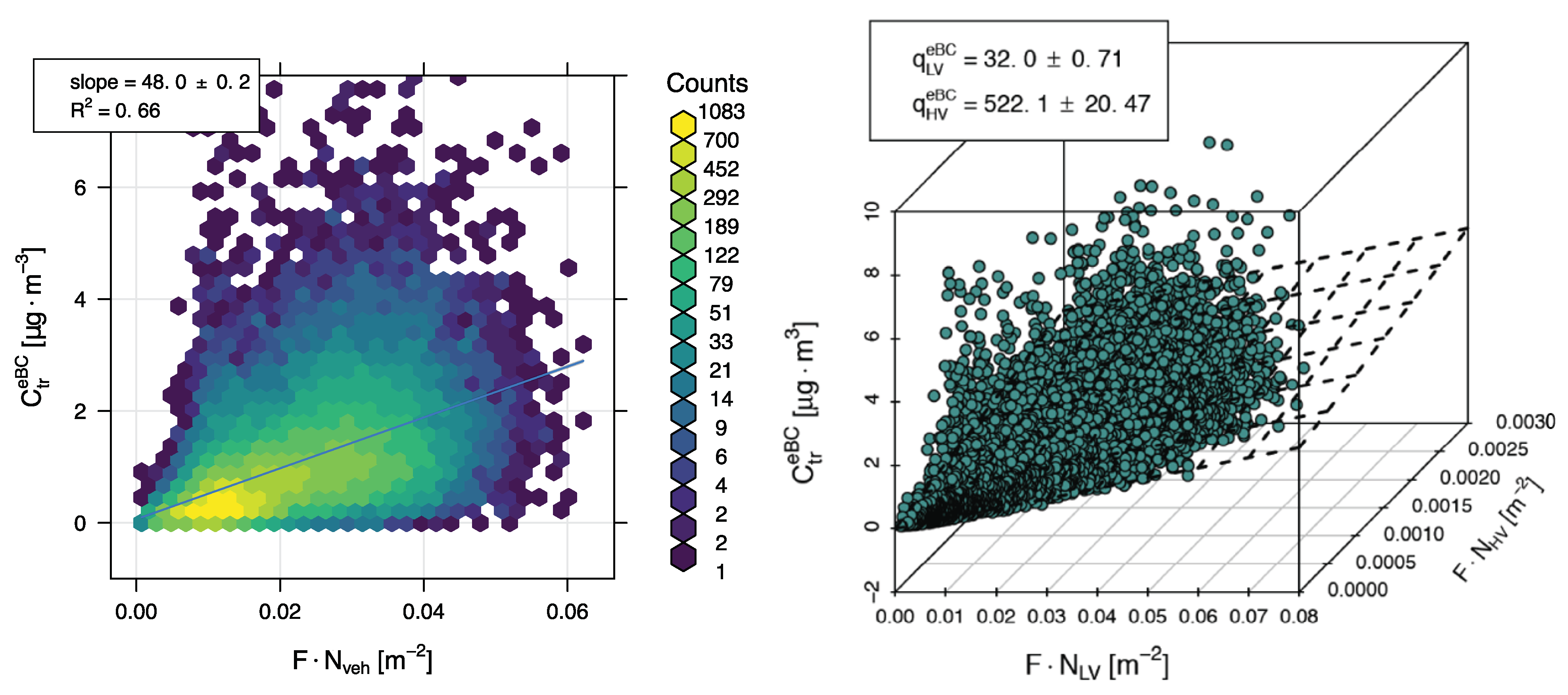
3.2.2. Deviation into Light and Heavy Traffic

As mentioned in Section 3.1, there is evidence that the share of heavy traffic within the fleet has a considerable influence on the fleet averaged EF. Being one of the few fleet parameters detectable, the EF can be split according to the type of vehicle, expecting that the mostly diesel-powered heavy vehicles emit considerably more BC. Figure 5 (right) shows the bivariate approach according to Equation (4). With the dilution factor times the number of vehicles in the light and heavy class on the x and y-axis, respectively, fitted against the eBC traffic increment on the z-axis, the slopes of the fitted plane correspond to the EFs. For the light vehicles this results in 32 mg km${}^{-1}$ and for the heavy vehicles in 522 mg km${}^{-1}$. The uncertainty given in the plot is merely the standard deviation of the regression. For the overall uncertainty of the EFs we can only give the qualitative statement, that it must be expected considerably higher (see discussion). These values are in line with findings from other studies, according to which the EF of heavy vehicles is about one order of magnitude higher than that of light vehicles.

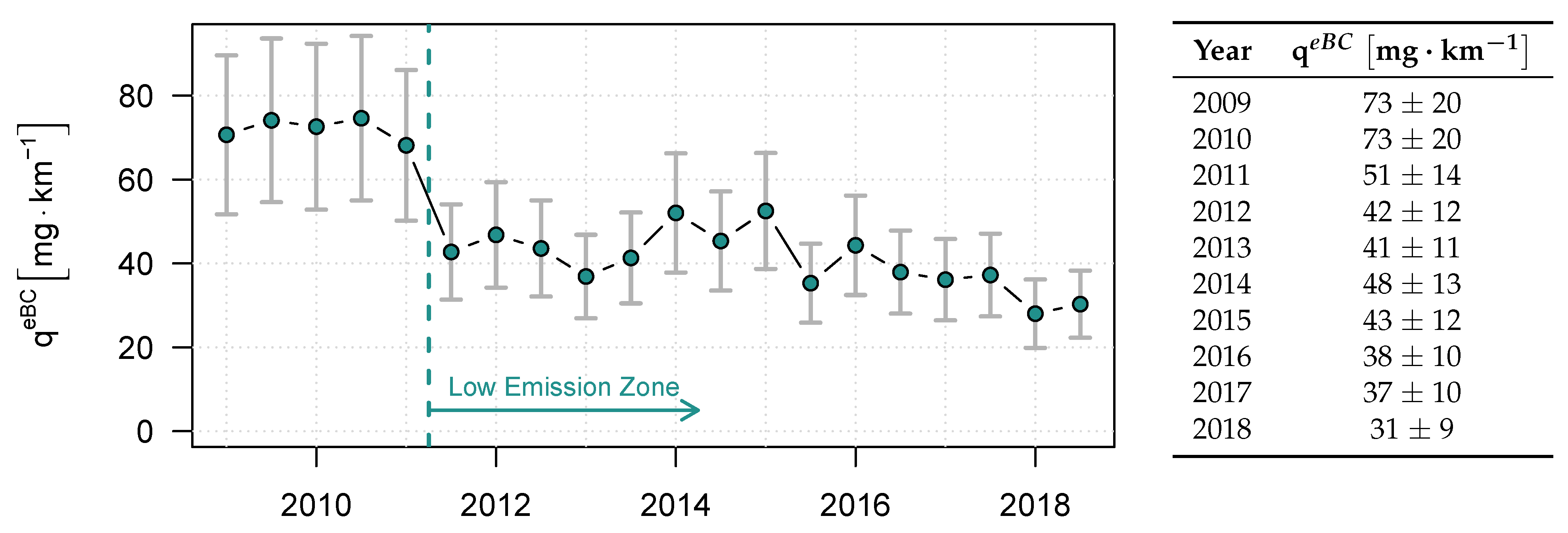
3.2.3. Seasonal Emission Factors and Trend

Since the composition of the fleet is constantly changing, it is of great interest, how the emission factor develops over time. As a measure of accelerating the renewal of the fleet, a low emission zone was introduced to the city of Leipzig which is expected to have significant influence on the EF. Covering most of the city area, it was installed in 2011 to ban all vehicles with high emissions. Allowed (“green emission sticker”) are gasoline vehicles and diesel powered ones with Euro 5 and higher or Euro 3 and 4 with DPFs [27]. In Figure 6 the weekly cycle of the median eBC traffic increment was split into the years 2009 to 2018. It already shows a significant trend towards lower traffic emissions, especially during the times with high traffic density. Only in the most recent years, especially 2018, there was again a slight increase during Friday evenings and the weekend. This might be attributed to a development in the neighbourhood of the EIBA station enhancing the busyness at leisure dominated times. During the day, the peak values decrease from around 2 $\mathsf{\mu }$g m${}^{-3}$ to below 1 $\mathsf{\mu }$g m${}^{-3}$. However, how does that translate into EFs? To analyse the long time series in still statistically relevant segments, the emission factors were averaged over half year periods. The summer was chosen from April to September, the winter from October to March. Figure 7 (left) shows the trend of the 6-month-fitted EFs. At the EIBA station the EF starts at over 70 mg km${}^{-1}$ in 2009. After the low emission zone, introduced on 1 March 2011 (vertical line), the eBC EF significantly decreased to below 50 mg km${}^{-1}$ (p-value < 2.2$·{10}^{-16}$). In the following years the value slowly decreases further to 30–40 mg km${}^{-1}$. On the right hand side Figure 7 also includes a table with the yearly fitted eBC EFs. For both yearly and half yearly EFs, an uncertainty is estimated comprised of the 95% confidence interval of the linear regression (around 2% for each period) plus an 25% uncertainty resulting from the error estimates described within the discussion part.

As for seasonality, one could expect that the EFs are higher in winter due to cold start effects or a higher traffic density we can not account for. Monthly segregated, our data merely shows a mild trend to lower values in winter. As mentioned in Section 2.1, the robustness of the increment method largely depends on the input data. To analyse the possible seasonal variance, we tested on selecting only the data pairs where the roadside signal was well above the background signal (like this excluding for example night time values or measurements at the windward side of the vortex). Applying such a “plausibility filter”, any seasonal effects become indistinguishable. We conclude that there is no seasonality detectable within this dataset. Only very few other studies assessed a seasonal variation for carbonaceous PM at all, since often the studies are based on short term experiments in the order of weeks or months. While for NO${}_x$ the evidence is increasingly strong that there are higher emission factors in winter [28], for carbonaceous particulates the trend is not clear. Ketzel et al. [29] found a significant seasonality for PM EFs with up to 45% lower values in summer than the annual average at stations in Finland and Sweden, while for stations in Germany, Austria and Denmark they found much lower variability of 5–10%. They are attributing this mainly to the different meteorological conditions and the use of studded tyres in the northern countries. For fuel based EFs of BC Saha et al. [30] as well as Wang et al. [31] found no statistically significant seasonality, but also observed a tendency toward higher values in summer. This would comply with our findings.

3.3. Discussion and Outlook

The results of studies focusing on the determination of EFs are highly variable, which can be influenced by the choice of method, but certainly by the circumstances like regional characteristics of the fleet (for real world EFs), or the choice of vehicles (for approaches on an individual level), the time frame in which they are carried out and local conditions. Inevitably, the type approval emission test results will have to be below the emission standard level for PM, which is 4.5 mg km${}^{-1}$ (for those vehicles where they have to be applied, see Introduction and [6]). To best compare our study with other real world approaches, we tried to pick studies on the same unit basis (distance travelled, while other studies calculate fuel based EFs) as well as similar locations (EFs from developing countries are often highly elevated [32]). This greatly limits the amount of comparable publications. Some exemplary studies deriving EFs for black or elemental carbon and other pollutants are summarised in

Table 1. Black carbon (BC)/ elemental carbon (EC) emission factors derived from different studies (Yom = year of measurement) and calculated from the Handbook Emission Factors for Road Transport (HBEFA). EFs, if available, are given for the mixed fleet vehicle and/or light vehicle & heavy vehicle. HBEFA distinguishes between passenger cars (PC) and light commercial vehicles (LCV).

Study	Yom	Country	Site	Parameter	Emission Factor [mg km${}^{-1}$]
					Mixed	LV	HV
Weingartner et al. [33]	1993	Switzerland	freeway tunnel	BC		1.6	122.7
Hueglin et al. [34]	2004	Switzerland	highway	EC	21
Keuken et al. [35]	2008	Netherlands	urban street	EC		30	190
Imhof et al. [37]	2002	Switzerland	urban street	BC	35	10	427
Krecl et al. [36]	2006	Sweden	street canyon	BC		gasoline: 11
						diesel: 94.8
	2013					gasoline: 2.5
						diesel: 23.4
HBEFA 4.1 [38]	2009	Germany	various	BC		PC: 8.7	95.5
	−2018					LCV: 52.1
This study	2009	Germany	street canyon	BC	48	32	522
	−2018

. Weingartner et al. [33] calculated EFs from measurements taken 1993 in a freeway tunnel in Switzerland. They found values of 1.6 mg km${}^{-1}$ for light vehicles and 122.7 mg km${}^{-1}$ for heavy vehicles in PM${}_3$. Hueglin et al. [34] retrieved EFs for EC from 2004 highway measurements. They classified roadside measurement data into ‘background’ and ‘traffic influenced’ according to the wind direction in 3-month-periods. For the mixed fleet they found an EF of 21 mg km${}^{-1}$. For a health impact assessment Keuken et al. [35] used fixed dynamometer derived ratios of EC to PM and applied them onto PM emission factors. For 2008 they calculated an EF of 30 mg km${}^{-1}$ for light duty vehicles (LDV, 50% diesel) and 190 mg km${}^{-1}$ for heavy duty vehicles (HDV). Krecl et al. [36] used a similar general approach as the one in our study, calculating the EF from the traffic increment, the traffic rate and a dilution rate. The dilution rate and the traffic increment though, they derived from measured NO${}_x$ concentrations and presumably known NO${}_x$ emission factors. They calculated the dilution rate and assumed that this would be the same for any other inert tracer like BC and PN. The traffic increment was derived from positive matrix factorization, dividing the concentrations into gasoline, diesel and background contributions. Imhof et al. [37] also retrieved the dilution rate via NO${}_x$ concentrations. The traffic increment they calculated from up- and downwind pollutant concentrations. For a station similar to our roadside station with stop-and-go-traffic in an urban setting they found a BC EF for the mixed fleet to be 35 mg km${}^{-1}$, for LDV 10 mg km${}^{-1}$ and for HDV 427 mg km${}^{-1}$. EFs for BC can also be retrieved from the Handbook of Emission Factors for Road Transport (HBEFA), Version 4.1 [38]. Chosen for comparison to this study were the categories light commercial vehicles (LCV, <3.5 t) and passenger cars (PC) as well as heavy duty vehicles (HDV, >3.5 t). The EF for BC (exhaust) plus BC (non-exhaust) was calculated for the modelled years 2009 to 2018 for a saturated traffic scenario of a collecting road with a speed limit of 50 km h${}^{-1}$. The resulting EFs were decreasing for all categories over the selected years, ranging from 14.1 to 4.7 mg km${}^{-1}$, 88.2 to 21.3 mg km${}^{-1}$ and 165.3 to 40.7 mg km${}^{-1}$ for PC, LCV and HDV, respectively. The averaged HBEFA EFs for BC are included in the table. Our study is certainly at the upper end of the range of these literature values. While for the light vehicle segment, they are only slightly higher than the comparable values, the heavy traffic segment stands out even a bit more. Various points can come together to produce the differences between these studies. One would be the method of retrieving the value for the carbonaceous particulate matter. Though BC and EC are closely related, the correlation between optically and thermally retrieved parameters can change depending on the location, time and instruments used [39]. Even though we selected only European studies for comparison, the fleet composition can vary greatly. Within German federal states the shares of the various power trains is already different (KBA [26]). Especially the traffic situation with the close junction and traffic lights could greatly influence our results due to idling cars and trucks which still can emit a considerable amount of particles [40]. The different probing of vehicles could influence the comparison to the HBEFA values, which are based on emission tests of individual vehicles. HBEFA tries to compensate this problem by probing vehicles with different mileages, applying multiple driving cycles and a wide range of combinations within the engine map. But still, this approach is limited to a selection and must not necessarily represent all aspects of the present driving fleet.

However, the method used in this study also has its limitations and the results are to be treated with appropriate caution. We here attempt a detailed error analysis. Apart from aforementioned measurement uncertainties, especially the limitations of the OSPM dispersion model may lead to discrepancies between the real and the estimated EFs. The OSPM is a generally well evaluated model. By comparing modelled and measured data, Ketzel et al. [41] showed in a reanalysis study, that the model produces reliable results when applied on an appropriate street geometry. For regular street canyons they found the results to be “generally well reproduced” over all wind directions. However, the OSPM is always an approximation to the real topography and lacks some features, that could have more or less influence on the calculated emission factors. These include for example the missing consideration of intersecting streets in the vicinity as additional sources of pollution, in our case especially the Herman-Liebmann-Straße with considerable traffic. This is most likely also the reason why there can be found a distinct dependence of the EF on the wind direction. Not accounting for the intersecting traffic may lead to an overestimation of the EF of up to 100% for the concerned wind directions assuming a comparable amount of traffic in both streets. Averaged over all wind directions, the overestimation of the EF would of course not be as grave. Another source of uncertainty might be the nearby traffic light. The model assumes a constant traffic flow and does not account for the resulting stop-and-go-traffic. Accepting idling emissions as part of an EF for stop-and-go traffic scenarios, this might only be a minor issue, mainly affecting very low wind speeds, when most of the turbulence is generated by the moving traffic. Other effects may concern the flow regime. At the corners of the buildings over the entire height, vortices can develop, transporting the tracer towards the mid of the building length [42]. In combination with the intersecting road this could lead to considerable uncertainties. Other meteorological conditions, such as thermal convection, which is not considered in OSPM, may also influence the dispersion of pollutants. Earlier studies at the same site though showed no significant effects: Klose et al. [43] tested a dataset of particle number measurements collected in EIBA for temperature and solar radiation dependence. They only found fluctuations within the standard deviation between sunny and non-sunny conditions. A negative correlation of particle number and temperature could only be ascribed to new particle formation of condensable vapours in traffic exhaust. A highly critical point in calculating the trend is the constant traffic profile calculated from data collected in 2005. Even though this was evaluated with manually counted 2015 data, certain fluctuations in traffic density in between may not be covered. Since there were no profound changes in traffic guidance around the station, we consider it reasonable to use the constant profile. However, every tendency towards less vehicles would cause an underestimation in the emission factor and vice versa. Uncertainties mostly affect the fleet split which is highly sensitive to the changes in the fractions. An attempt to correct the traffic density with data of other counting stations was discarded (see Appendix A).

A qualitative assessment of the precision of the estimated EF is hard to achieve. While for certain parameters more or less fixed uncertainties can be assumed, the model (usage) as a source of error is much harder to consider. For measurements of the MAAP we adapt the variance found by Müller et al. [25] of about 5%. Within the vehicle counts we only see very small variation. However, since we cannot account for changes between the years, we also propose a ±10% range for this parameter. A general hint on the uncertainty of the OSPM model in the literature is not to be found and would anyway vary greatly with the setup of the domain, depending, among others, on the suitability of the station for this model. A detailed sensitivity study would hold way too many options to be feasible. Some parameters can be directly tested varying the input into the model. This certainly is true for the meteorology. Rounding up the manufacturers information on the measurement uncertainty, the wind speed (ws) is varied by ±5% and the wind direction (wd) by ±5${}^{\circ }$. In the case of increased wind speed the dilution factor (DF) decreases by about 2.5% (averaged over the whole dataset), meaning stronger dilution. Decreasing the wind speed −5% results in an increased DF by 2.5% (weaker dilution). The upper row of Figure 8 shows the deviation from the original DF revealing a range of ±10% for the different combinations of wind speed and direction. The histograms in the lower row give an impression of the share of deviation from the original DFs. Varying the wind direction accordingly in the model input, we see a much larger range of more than ±20% (Figure 8, upper row). But it nearly averages out, applied to the hole dataset, with a tendency towards decreased DF for wd +5${}^{\circ }$ (−0.2%) and increased DF (+0.6%) for wd −5%. This though would be different if the prevailing regional wind pattern would be different (compare wind rose in Figure 2). Assuming similar deviation for other parameters like street orientation (which in fact corresponds to a change in wind direction), receptor and building height or street width, we propose another 10% uncertainty for the model related DF.

In the end it should be kept in mind, that this method has a profound uncertainty. It must be assumed, however, that other studies struggle with similar scales of uncertainties. It would be interesting to compare different methods for same stations or on the other hand the same method to different stations. The latter was tried to achieve as part of the project this study originated from [44], comparing two additional stations with the same approach. The resulting eBC EFs were similarly high, but the conditions were still hard to compare since the topography was significantly different from the street canyon topography required for the OSPM model. Because of that reason, the presented study focuses on the EIBA station. A re-evaluation of the dataset with a CFD model which can handle some of these drawbacks is planned for the near future.

4. Summary and Conclusions

This study is an attempt to estimate vehicle emission factors for black carbon under realistic conditions. With an inverse modelling approach, using the well known, easy to handle OSPM (Operational Street Pollution Model) we analysed a series of 10 years of measurement data. The reported values are derived—and therefore to be considered representative—only for inner city traffic on a rather congested road with traffic lights. Averaged over the entire available period, we found an eBC EF of 48 mg km${}^{-1}$ for a vehicle of the mixed fleet. Segregation into light (<3.5 t) and heavy (>3.5 t) vehicles yielded 32 and 522 mg km${}^{-1}$, respectively. These values are well above the emission standard limits for Euro 5 and 6 for PM and also above comparable EFs extracted from the HBEFA 4.1 database. Nevertheless, against the tendency of rising shares of diesel powered vehicles and direct injection engines, the emission factors decrease. Starting the observed time span with 70 mg km${}^{-1}$, the eBC EF amounts to only around 30–40 mg km${}^{-1}$ after a few years. Apparently, the improvement in technology overrules any opposing trends to a considerable degree. Administrative measures, like the introduction of a low emission zone, are found to be a useful tool to vastly accelerate these developments on a short term basis. A seasonal trend could not be found.

References

1. Pant, P.; Harrison, R.M. Estimation of the contribution of road traffic emissions to particulate matter concentrations from field measurements: A review. Atmos. Environ. 2013, 77, 78–97. [Google Scholar] [CrossRef]
2. Krzyżanowski, M.; Kuna-Dibbert, B.; Schneider, J. Health Effects of Transport-Related Air Pollution; WHO Regional Office Europe: Copenhagen, Denmark, 2005. [Google Scholar]
3. Bond, T.C.; Doherty, S.J.; Fahey, D.W.; Forster, P.M.; Berntsen, T.; DeAngelo, B.J.; Flanner, M.G.; Ghan, S.; Kärcher, B.; Koch, D.; et al. Bounding the role of black carbon in the climate system: A scientific assessment. J. Geophys. Res. Atmos. 2013, 118, 5380–5552. [Google Scholar] [CrossRef]
4. Grahame, T.J.; Schlesinger, R.B. Cardiovascular health and particulate vehicular emissions: A critical evaluation of the evidence. Air Qual. Atmos. Health 2010, 3, 3–27. [Google Scholar] [CrossRef] [PubMed] [Green Version]
5. Janssen, N.A.; Hoek, G.; Simic-Lawson, M.; Fischer, P.; Van Bree, L.; Ten Brink, H.; Keuken, M.; Atkinson, R.W.; Anderson, H.R.; Brunekreef, B.; et al. Black carbon as an additional indicator of the adverse health effects of airborne particles compared with PM10 and PM2. 5. Environ. Health Perspect. 2011, 119, 1691. [Google Scholar] [CrossRef] [Green Version]
6. European Commission. Commission Regulation (EC) No 692/2008 of 18 July 2008 implementing and amending Regulation (EC) No 715/2007 of the European Parliament and of the Council on type-approval of motor vehicles with respect to emissions from light passenger and commercial vehicles (Euro 5 and Euro 6) and on access to vehicle repair and maintenance information. Off. J. Eur. Union 2008, 199, 1–136. [Google Scholar]
7. Weiss, M.; Bonnel, P.; Hummel, R.; Provenza, A.; Manfredi, U. On-Road Emissions of Light-Duty Vehicles in Europe. Environ. Sci. Technol. 2011, 45, 8575–8581. [Google Scholar] [CrossRef]
8. Peitzmeier, C.; Loschke, C.; Wiedenhaus, H.; Klemm, O. Real-world vehicle emissions as measured by in situ analysis of exhaust plumes. Environ. Sci. Pollut. Res. 2017, 24, 23279–23289. [Google Scholar] [CrossRef] [Green Version]
9. Matzer, C.; Weller, K.; Dippold, M.; Lipp, S.; Röck, M.; Rexeis, M.; Hausberger, S. Update of Emission Factors for HBEFA Version 4.1; Final Report; I-05/19/CM EM-I-16/26/679; Graz University of Technology: Graz, Austria, 2019. [Google Scholar]
10. Caroca, J.C.; Millo, F.; Vezza, D.; Vlachos, T.; De Filippo, A.; Bensaid, S.; Russo, N.; Fino, D. Detailed Investigation on Soot Particle Size Distribution during DPF Regeneration, using Standard and Bio-Diesel Fuels. Ind. Eng. Chem. Res. 2011, 50, 2650–2658. [Google Scholar] [CrossRef]
11. Kadijk, G.; Elstgeest, M.; Ligterink, N.; Mark, P. Investigation into a Periodic Technical Inspection (PTI) Test Method to Check for Presence and Proper Functioning of Diesel Particulate Filters in Light-Duty Diesel Vehicles Part 2; Technical Report; TNO: Den Haag, The Netherlands, 2017. [Google Scholar]
12. Kontses, A.; Triantafyllopoulos, G.; Ntziachristos, L.; Samaras, Z. Particle number (PN) emissions from gasoline, diesel, LPG, CNG and hybrid-electric light-duty vehicles under real-world driving conditions. Atmos. Environ. 2020, 222, 117126. [Google Scholar] [CrossRef]
13. Saliba, G.; Saleh, R.; Zhao, Y.; Presto, A.A.; Lambe, A.T.; Frodin, B.; Sardar, S.; Maldonado, H.; Maddox, C.; May, A.A.; et al. Comparison of Gasoline Direct-Injection (GDI) and Port Fuel Injection (PFI) Vehicle Emissions: Emission Certification Standards, Cold-Start, Secondary Organic Aerosol Formation Potential, and Potential Climate Impacts. Environ. Sci. Technol. 2017, 51, 6542–6552. [Google Scholar] [CrossRef]
14. Zimmerman, N.; Wang, J.M.; Jeong, C.H.; Ramos, M.; Hilker, N.; Healy, R.M.; Sabaliauskas, K.; Wallace, J.S.; Evans, G.J. Field Measurements of Gasoline Direct Injection Emission Factors: Spatial and Seasonal Variability. Environ. Sci. Technol. 2016, 50, 2035–2043. [Google Scholar] [CrossRef] [PubMed]
15. Park, S.S.; Kozawa, K.; Fruin, S.; Mara, S.; Hsu, Y.K.; Jakober, C.; Winer, A.; Herner, J. Emission Factors for High-Emitting Vehicles Based on On-Road Measurements of Individual Vehicle Exhaust with a Mobile Measurement Platform. J. Air Waste Manag. Assoc. 2011, 61, 1046–1056. [Google Scholar] [CrossRef] [PubMed] [Green Version]
16. Mensch, P.V.; Cuelenaere, R.; Ligterink, N.; Kadijk, G. Update: Assessment of risks for elevated emissions of vehicles under the boundaties of RDE. In Identifying Relevant Driving and Vehicle Conditions and Possible Abatement Measures; TNO: Den Haag, The Netherlands, 2019. [Google Scholar]
17. European Commission. Commission Regulation (EU) 2016/427 of 10 March 2016 Amending Regulation (EC) No 692/2008 as Regards Emissions from Light Passenger and Commercial Vehicles (Euro 6); European Commission: Brussels, Belgium, 2016. [Google Scholar]
18. Franco, V.; Kousoulidou, M.; Muntean, M.; Ntziachristos, L.; Hausberger, S.; Dilara, P. Road vehicle emission factors development: A review. Atmos. Environ. 2013, 70, 84–97. [Google Scholar] [CrossRef]
19. Petzold, A.; Ogren, J.A.; Fiebig, M.; Laj, P.; Li, S.M.; Baltensperger, U.; Holzer-Popp, T.; Kinne, S.; Pappalardo, G.; Sugimoto, N.; et al. Recommendations for reporting “black carbon” measurements. Atmos. Chem. Phys. 2013, 13, 8365–8379. [Google Scholar] [CrossRef] [Green Version]
20. Ketzel, M.; Wåhlin, P.; Berkowicz, R.; Palmgren, F. Particle and trace gas emission factors under urban driving conditions in Copenhagen based on street and roof-level observations. Atmos. Environ. 2003, 37, 2735–2749. [Google Scholar] [CrossRef]
21. Lenschow, P.; Abraham, H.J.; Kutzner, K.; Lutz, M.; Preuß, J.D.; Reichenbächer, W. Some ideas about the sources of PM10. Atmos. Environ. 2001, 35, S23–S33. [Google Scholar] [CrossRef]
22. Berkowicz, R.; Hertel, O.; Larsen, S.E.; Sørensen, N.N.; Nielsen, M. Modelling Traffic Pollution in Streets; National Environmental Research Institute: Roskilde, Denmark, 1997; Volume 10129, p. 20.
23. Van Pinxteren, D.; Fomba, K.W.; Spindler, G.; Muller, K.; Poulain, L.; Iinuma, Y.; Loschau, G.; Hausmann, A.; Herrmann, H. Regional air quality in Leipzig, Germany: Detailed source apportionment of size-resolved aerosol particles and comparison with the year 2000. Faraday Discuss. 2016, 189, 291–315. [Google Scholar] [CrossRef]
24. Petzold, A.; Schönlinner, M. Multi-angle absorption photometry—A new method for the measurement of aerosol light absorption and atmospheric black carbon. J. Aerosol Sci. 2004, 35, 421–441. [Google Scholar] [CrossRef]
25. Müller, T.; Henzing, J.S.; De Leeuw, G.; Wiedensohler, A.; Alastuey, A.; Angelov, H.; Bizjak, M.; Coen, M.C.; Engstrom, J.E.; Gruening, C.; et al. Characterization and intercomparison of aerosol absorption photometers: Result of two intercomparison workshops. Atmos. Meas. Tech. 2011, 4, 245–268. [Google Scholar] [CrossRef] [Green Version]
26. Kraftfahrt-Bundesamt. Bestand an Kraftfahrzeugen Nach Umwelt-Merkmalen. Available online: https://www.kba.de/DE/Statistik/Produktkatalog/produktkatalog_node.html (accessed on 8 December 2020).
27. City of Leipzig. Questions and Answers Regarding the Environmental Zone. Available online: https://english.leipzig.de/environment-and-transport/environmental-zone/ (accessed on 3 November 2020).
28. Li, X.; Dallmann, T.R.; May, A.A.; Presto, A.A. Seasonal and Long-Term Trend of on-Road Gasoline and Diesel Vehicle Emission Factors Measured in Traffic Tunnels. Appl. Sci. 2020, 10, 2458. [Google Scholar] [CrossRef] [Green Version]
29. Ketzel, M.; Omstedt, G.; Johansson, C.; Düring, I.; Pohjola, M.; Oettl, D.; Gidhagen, L.; Wåhlin, P.; Lohmeyer, A.; Haakana, M.; et al. Estimation and validation of PM2.5/PM10 exhaust and non-exhaust emission factors for practical street pollution modelling. Atmos. Environ. 2007, 41, 9370–9385. [Google Scholar] [CrossRef]
30. Saha, P.K.; Khlystov, A.; Snyder, M.G.; Grieshop, A.P. Characterization of air pollutant concentrations, fleet emission factors, and dispersion near a North Carolina interstate freeway across two seasons. Atmos. Environ. 2018, 177, 143–153. [Google Scholar] [CrossRef]
31. Wang, J.M.; Jeong, C.H.; Zimmerman, N.; Healy, R.M.; Evans, G.J. Real world vehicle fleet emission factors: Seasonal and diurnal variations in traffic related air pollutants. Atmos. Environ. 2018, 184, 77–86. [Google Scholar] [CrossRef]
32. Madueño, L.; Kecorius, S.; Birmili, W.; Müller, T.; Simpas, J.; Vallar, E.; Galvez, M.C.; Cayetano, M.; Wiedensohler, A. Aerosol Particle and Black Carbon Emission Factors of Vehicular Fleet in Manila, Philippines. Atmosphere 2019, 10, 603. [Google Scholar] [CrossRef] [Green Version]
33. Weingartner, E.; Keller, C.; Stahel, W.; Burtscher, H.; Baltensperger, U. Aerosol emission in a road tunnel. Atmos. Environ. 1997, 31, 451–462. [Google Scholar] [CrossRef]
34. Hueglin, C.; Buchmann, B.; Weber, R.O. Long-term observation of real-world road traffic emission factors on a motorway in Switzerland. Atmos. Environ. 2006, 40, 3696–3709. [Google Scholar] [CrossRef]
35. Keuken, M.; Zandveld, P.; van den Elshout, S.; Janssen, N.A.; Hoek, G. Air quality and health impact of {PM10} and {EC} in the city of Rotterdam, the Netherlands in 1985–2008. Atmos. Environ. 2011, 45, 5294–5301. [Google Scholar] [CrossRef]
36. Krecl, P.; Johansson, C.; Targino, A.C.; Ström, J.; Burman, L. Trends in black carbon and size-resolved particle number concentrations and vehicle emission factors under real-world conditions. Atmos. Environ. 2017, 165, 155–168. [Google Scholar] [CrossRef]
37. Imhof, D.; Weingartner, E.; Ordóñez, C.; Gehrig, R.; Hill, M.; Buchmann, B.; Baltensperger, U. Real-World Emission Factors of Fine and Ultrafine Aerosol Particles for Different Traffic Situations in Switzerland. Environ. Sci. Technol. 2005, 39, 8341–8350. [Google Scholar] [CrossRef]
38. INFRAS. Handbook Emission Factors from Road Transport (HBEFA) 4.1; INFRAS: Zurich, Switzerland, 2019. [Google Scholar]
39. Salako, G.O.; Hopke, P.K.; Cohen, D.D.; Begum, B.A.; Biswas, S.K.; Pandit, G.G.; Lodoysamba, S.; Wimolwattanapun, W.; Bunprapob, S.; Chung, Y.S.; et al. Exploring the Variation between EC and BC in a Variety of Locations. Aerosol Air Qual. Res. 2012, 12, 1–7. [Google Scholar] [CrossRef]
40. Giechaskiel, B.; Lähde, T.; Suarez-Bertoa, R.; Valverde, V.; Clairotte, M. Comparisons of Laboratory and On-Road Type-Approval Cycles with Idling Emissions. Implications for Periodical Technical Inspection (PTI) Sensors. Sensors 2020, 20, 5790. [Google Scholar] [CrossRef] [PubMed]
41. Ketzel, M.; Jensen, S.S.; Brandt, J.; Ellermann, T.; Olesen, H.R.; Berkowicz, R.; Hertel, O. Evaluation of the street pollution model OSPM for measurements at 12 streets stations using a newly developed and freely available evaluation tool. J. Civ. Environ. Eng. 2012, 1. [Google Scholar] [CrossRef] [Green Version]
42. Hoydysh, W.G.; Dabberdt, W.F. Kinematics and dispersion characteristics of flows in asymmetric street canyons. Atmos. Environ. 1988, 22, 2677–2689. [Google Scholar] [CrossRef]
43. Klose, S.; Birmili, W.; Voigtländer, J.; Tuch, T.; Wehner, B.; Wiedensohler, A.; Ketzel, M. Particle number emissions of motor traffic derived from street canyon measurements in a Central European city. Atmos. Chem. Phys. 2011, 9, 3763–3809. [Google Scholar] [CrossRef]
44. Pfeifer, S.; Wiesner, A.; Wehner, B.; Alas, H.D.; Chen, Y.; Wiedensohler, A. Einfluss von Ruß auf Luftqualität und Klimawandel; Final Report; Landesamt für Umwelt, Landwirtschaft und Geologie: Dresden, Germany, 2018. [Google Scholar]
45. R Core Team. R: A Language and Environment for Statistical Computing; R Foundation for Statistical Computing: Vienna, Austria, 2019. [Google Scholar]
46. Carslaw, D.C.; Ropkins, K. Openair—An R package for air quality data analysis. Environ. Model. Softw. 2012, 27–28, 52–61. [Google Scholar] [CrossRef]
47. Garnier, S. Viridis: Default Color Maps from ‘Matplotlib’. R Package Version 0.5.1. 2018. Available online: https://github.com/sjmgarnier/viridis (accessed on 8 May 2020).
48. Meschiari, S. Latex2exp: Use LaTeX Expressions in Plots. R Package Version 0.4.0. 2015. Available online: http://github.com/stefano-meschiari/latex2exp (accessed on 8 May 2020).
49. Ligges, U.; Mächler, M. Scatterplot3d—An R Package for Visualizing Multivariate Data. J. Stat. Softw. 2003, 8, 1–20. [Google Scholar] [CrossRef] [Green Version]
Figure 1. Left: Scheme of a street canyon with indicated vortex. Right: North-oriented GoogleEarth(c) picture of the street canyon with marked station Eisenbahnstraße (EIBA).
Atmosphere 12 00031 g001
Figure 2. Left: Location of the measurement stations within the city (red: roadside station; yellow: urban background station). Additionally, the border of the low emission zone (LEZ) is included as blue line. The wind rose shows the wind speed (color scale) as frequency according to wind direction. Right: Correlation of the measured eBC concentration C e B C for the urban background stations TROPOS and Leipzig West.
Atmosphere 12 00031 g002
Figure 3. Fixed traffic profile ((a): light vehicles and heavy vehicles *10, for visibility) and weekly patterns of the median dilution factor F (b), black carbon concentration at the background and the roadside stations (c), black carbon traffic increment (d), and estimated vehicle emission factor for black carbon (e).
Atmosphere 12 00031 g003
Figure 4. Polar display of the dilution factor (left) and the traffic increment of the measured BC concentration, normalized by the traffic density (right). The monitoring roadside station is located at the northern wall of the street canyon.
Atmosphere 12 00031 g004
Figure 5. Left: Density plot of the linear regression: total number of vehicles ( N v e h ) times dilution factor (F) against the eBC traffic increment ( C t r e B C ); Right: Bivariate regression of the number of light and heavy vehicles ( N L V & N H V ) times the dilution factor against the eBC traffic increment. Slopes of the fitting plane correspond to the emission factors q L V e B C and q H V e B C .
Atmosphere 12 00031 g005
Figure 6. Weekly cycle of the median eBC traffic increment C t r e B C split into the years 2009 to 2018.
Atmosphere 12 00031 g006
Figure 7. Left: eBC emission factor for the station EIBA as summer/winter averages 2009–2018 from 6-month scatter plots. Error bars indicate 95% confidence interval of the fit plus 25% measurement uncertainty (see discussion). Right: Table with the yearly fitted eBC emission factor.
Atmosphere 12 00031 g007
Figure 8. Variation experiment with the Operational Street Pollution Model (OSPM). For the variation of the input parameters wind speed by 5% and the wind direction by ±5 , the output of the dilution factor F v a r in relation to the to the original dilution factor F o r i g i n a l is displayed. In the upper row the quotient is shown as polar plot, in the lower panel as histogram of the density.
Atmosphere 12 00031 g008