Selective foraging within estuarine plume fronts by an inshore resident seabird
 Nicole D. Kowalczyk1
  Richard D. Reina
- 1School of Biological Sciences, Monash University, Clayton, VIC, Australia
- 2Research Department, Phillip Island Nature Parks, Cowes, VIC, Australia
The distribution of predators relative to specific abiotic and biotic factors within estuarine plume fronts is largely unexplored due to the lack of fine-scale temporal and spatial oceanographic data. Defining preferred foraging conditions of seabirds in these areas is critical to identifying important foraging habitats. Here, we use data obtained from Ships of Opportunity to improve the way we quantify oceanographic conditions at scales that match marine animal foraging activities within these areas. Using biologgers and data from a Ship of Opportunity, we assessed the fine-scale habitat utilization of the Little Penguin (Eudyptula minor) within an estuarine plume in Victoria, Australia. We assessed how environmental conditions within the home-range (transit and foraging) and core-range (subset area of intensive foraging within the home-range) of this inshore seabird differed to environmental conditions in the accessible, but non-utilized range (i.e., non-foraging range). Penguin foraging ranges occurred in waters with higher Chl-a, turbidity, temperature and lower salinity than non-foraging ranges. High Chl-a biomass was the most important explanatory variable of penguin distribution. Environmental conditions between the core-range and less used home-range also differed. Waters in the core-range were less productive, less turbid and less dynamic. We suggest penguins are foraging in these core-ranges due to the productive yet stable environmental conditions that likely offer a higher degree of prey predictability than the fluctuating conditions in the wider home-range. Furthermore, penguins may spend a greater proportion of their time in core-ranges as these waters have relatively low turbidity and may improve the ability of penguins to detect and capture their prey. Our results highlight the ability of a small-ranging, visual predator to selectively forage in waters with favorable conditions at fine-scales as a potential means to improve foraging efficiency.
Introduction
Estuarine plume fronts are a type of frontal system formed by interactions between tidal processes and river flow with the physical interfaces between these water bodies manifesting as steep gradients in temperature, salinity and turbidity (Le Fèvre, 1987). Within these areas, mixing, and nutrient retention enhance primary productivity, which in turn attract and aggregate zooplankton (Grimes and Finucane, 1991). Entrainment of phytoplankton and zooplankton attract foraging fish, making estuarine plume fronts important nearshore foraging features for marine predators, particularly seabirds (Grimes and Kingsford, 1996; Skov and Prins, 2001; Zamon et al., 2014). However, the dynamic nature of these water masses result in large physical and physico-chemical fluctuations (e.g., temperature, salinity and dissolved oxygen), which influence local prey distribution, composition and biomass (Grimes and Finucane, 1991; Wagner and Austin, 1999). This variability has subsequent effects on the distribution of marine predators, whose at-sea distribution is mostly controlled by the occurrence of their prey as well as their physiological and breeding energetic constraints (Wakefield et al., 2009; Zamon et al., 2014).
Although estuarine plume fronts and plume regions are recognized as important nearshore foraging habitats, the distribution of seabirds relative to specific abiotic and biotic factors within these features is largely unexplored. Characterizing the environmental factors that define the foraging ranges of seabirds in these regions is important to identifying preferred foraging habitats and to understanding how changes in environmental conditions may impact their distribution. Further, this information can be used to investigate processes that influence the availability of prey (Tremblay et al., 2009; Zamon et al., 2014).
Advancements in bio-logging technologies and spatial/temporal analyses have enabled the estimation of preferred foraging locations (Wakefield et al., 2009). However, a key constraint in identifying fine-scale habitat preferences around estuarine plumes is the lack of data describing oceanographic processes at temporal-spatial scales that match the foraging activities of seabirds (Adams et al., 2010; Scales et al., 2014). Remotely sensed oceanographic data can be of relatively high spatial resolution, but temporal resolution is compromised by cloud cover and sun-glint masking surface waters (Shaffer et al., 2005; Wakefield et al., 2009). Additionally, satellite signals originate in surface layers and it is not usually possible to observe subsurface levels, and few platforms provide data that describe features on sub-mesoscale spatial scales that may be important to understand ocean mixing and nutrient supply (Joint and Groom, 2000; Evans et al., 2014). Ships of Opportunity are typically volunteer merchant vessels that carry a range of environment quality monitoring equipment used to sample seawater in their travel route. Data obtained from these Ships are one way to overcome oceanographic sampling limitations (Petersen et al., 2011). These vessels can provide high spatial and temporal resolution data regarding marine environments as series of transects along regularly scheduled routes, often having the capacity to measure suites of environmental data (Lee et al., 2011). Despite the high quality of data and wide distribution of these vessels, few studies have used their data in combination with the foraging ranges of seabirds to provide insights into the fine-scale mechanisms underlying animal-oceanography interactions (Joiris et al., 2013; Commins et al., 2014).
Kowalczyk et al. (2015a) identified the importance of a river plume in structuring the foraging distribution of an inshore seabird, the little penguin (Eudyptula minor). We build upon those findings to assess the fine-scale habitat utilization and foraging habitat preferences of penguins within the estuarine plume region. We used GPS biologgers and environmental data (turbidity, salinity, temperature, and Chl-a biomass), obtained from a Ship of Opportunity, to determine the fine-scale habitat preference of little penguins in relation to environmental factors within the plume region, during three breeding seasons. This information is vital to characterizing important foraging habitats within the bay and can be useful in investigating the processes that influence the accessibility of prey to predators within this coastal system (Tremblay et al., 2009). Specifically, we assessed: (1) how environmental conditions within the home-ranges (defined as areas of individuals' active use) of penguins differed to those in their core-ranges [the area(s) of intensive use within the home-range, where most foraging activity is expected to take place] (Kaufman, 1962; Ford and Krumme, 1979); and (2). how environmental conditions within the foraging ranges of penguins (comprised of core-ranges and home-ranges) differed to environmental conditions in the nearby, accessible, but non-utilized range (hereafter referred to as the non-foraging range).
Methods
Study Area
Port Phillip Bay encloses an area of approximately 1930 km2, with a mean depth of 13.6 m, although over half the bay is less than 8 m deep (Harris, 1996). The bay is joined to Bass Strait through a 3 km-wide channel and semi-diurnal tides comprising one large and one small tide each day enter the bay (Harris, 1996). Hydrodynamics within the bay are constrained by the small entrance and neighboring flood tidal sand banks that reduce tidal volumes by more than 90% and equate with long residence times (up to 2 years) in the bay (Lee et al., 2012). The Yarra River in the north and the Western Treatment Plant in the west provide the majority of freshwater inflow, which typically maintains a hyposaline environment, but during drought bay salinities can exceed ocean values (Lee et al., 2012). Catchment loadings primarily occur at the northern end of the bay and productivity (Chl-a and phytoplankton), turbidity and salinity gradients typically become less productive, less turbid and more saline toward the southern entrance (Longmore et al., 1999; Lee et al., 2012). The bay experiences a temperate oceanic climate with cool, wet winters (SST minimum of 7°C) and warm, dry summers (SST up to 25°C) (Sampson et al., 2014).
Several shipping channels exist in the north and west of the Bay, as well as the south where Port Phillip Bay joins Bass Strait (Preston et al., 2008). The Spirit of Tasmania, a Ship of Opportunity, transverses across the Port Melbourne Channel, which has a maintained depth of 10.9 m in the north and 15.9 m in the south (Port of Melbourne, 2013).
Bird Instrumentation and Tracking
Research was conducted under scientific permits issued by the Victorian Department of Environment and Primary Industries (10003374, 10003848, 10005601), and approved by the Animal Ethics Committee of Monash University (BSCI/2006/12, BSCI/2010/22, BSCI/2011/33). A single foraging trip for each of 57 individual penguins was tracked in the austral spring and summer of 2008 (n = 15), 2011 (n = 10), and 2012 (n = 32) from a breeding colony (approximately 400 breeding pairs) (Preston, 2010), on St Kilda breakwater, Victoria, Australia (−37.51°S, 144.57°E). Penguins were tracked during the guard breeding stage, when chicks are between 1–19 days old, and adults undertake 1-day foraging trips within a 30 km radius of their breeding site (Collins et al., 1999; Preston et al., 2008). In 2008, birds were weighed (±10 g) and equipped with mini-GPSloggers (Earth and Ocean Technologies, 46.5 × 16 mm, minimum cross sectional area 496 mm2, mass in air 29 g). In 2011 and 2012, penguins were weighed (±10 g) and equipped with CatTraq GT-120 GPS devices (Perthold Engineering LLC, 44.5 × 28.5 mm, minimum cross sectional area 371 mm2, mass in air 17 g) that were sealed in a heat-shrink rubber tube for waterproofing. Loggers were attached to the posterior dorsal region of the bird with Tesa® tape (Beiersdorf AG, GmbH, Hamburg, Germany) as per Wilson et al. (1997). Devices weighed a maximum of 3.6% of the bird's mass in air, and were therefore under the upper limit of logger/body mass ratios recommended for penguins (Ropert-Coudert et al., 2007). Loggers recorded position every 15 s from 4 a.m. to 9 p.m. to coincide with the daily foraging activities of penguins. After a single foraging trip (1 day), penguins were captured in their nests, and their loggers were removed. The dataset for the GPS locations of tracked birds is publicly available at https://oztrack.org/projects/195.
The 95% home-range contour area is considered to be the area of individuals' active use (home-range) whilst the 50% core-area is considered to be an area (or areas) of intensive use which is a subset within the home-range (Kaufman, 1962) where most of the foraging activity of a central place forager is expected to take place (Ford and Krumme, 1979). The home-range contour area (95% Kernal Utilization Distribution, smoothing factor = 7, grid = 2 km) and core-range contour area (50% Kernal Utilization Distribution, smoothing factor = 7, grid = 2 km) of penguins were calculated using the Adehabitat package in R (Calenge, 2006). We used a non-parametric fixed kernel density estimator to estimate the probability that individuals will be found at specific locations. The ad-hoc method was used to calculate the smoothing parameter. Additionally, the geographic coordinates of the accessible non-foraging range were defined as the area within 30 km (straight line distance) from the colony, excluding the home- and core-ranges. Therefore, for each penguin's track, three foraging characteristics were calculated: (i) core-range contour area (ii) home-range contour area, which together comprised the foraging range, and (iii) non-foraging range.
Environmental Conditions
The Spirit of Tasmania transits Port Phillip Bay on a daily basis. The autonomous sampling system aboard the vessel collects 10 s averages of surface water (0–6 m deep) parameters including salinity (Seabird SBE-45, resolution of 0.003 psu, hereafter psu), sea surface temperature (Seabird SBE-38, resolution of 0.0001°C, hereafter SST), chlorophyll-a fluorescence (WETLabs WETStar fluorometer, resolution of 0.02 μg/L, hereafter Chl-a), turbidity (WETLabs WETStar fluorometer, resolution of 0.02 nephelometric turbidity units, hereafter turbidity), and position (SBE interface box, 1/12° latitude and 1/12° longitude) along the Port Melbourne Channel in Port Phillip Bay. Data have been collected by the ferry since 2008 and uploaded into the national Integrated Marine Observing System (www.imos.org.au) for broader distribution. In 2012, no data were uploaded to IMOS due to technical maintenance of the autonomous sampling system aboard the vessel. The dataset for the variables used is publicly available at https://imos.aodn.org.au/imos123/home?uuid=02640f4e-08d0-4f3a-956b-7f9b58966ccc
Statistical Analysis
In 2008 (n = 11), 2011 (n = 5), and 2012 (n = 11), the core- and home-range of 27 penguins overlapped with the Spirit of Tasmania shipping channel (Figures 1A,B). To quantify differences in environmental conditions within the foraging and non-foraging ranges of individual penguins we extracted psu, SST, Chl-a, and turbidity values from within the latitudinal gradient of the (i) core-range, (ii) home-range and (iii) non-foraging range for each of the 16 penguins tracked in 2008 and 2011 (no Spirit of Tasmania data were available in 2012). There is high variability in environmental conditions between years, as expected within a bay system like our study site and we have reported this inter-annual variability in previous studies (Preston et al., 2010; Kowalczyk et al., 2014, 2015b). As our aim was to compare penguins' area usage between core-ranges and home-ranges in relation to environmental conditions, we analyzed each year separately to avoid this large, confounding effect. For each year, generalized linear modeling (GLMM) with a gamma distribution was used to identify environmental differences between the home-range, core-range, and non-foraging range of penguins. Linear mixed-effect models using the “nlme” package for R (Pinheiro et al., 2013) were used to determine environmental differences between ranges where environmental parameters (psu, SST, Chl-a, turbidity) were treated as the response variables, foraging range (home-range, core-range, non-foraging range) as the fixed effect and individuals as a random factor. We used model selection to choose the best fitted model based on the lowest AICc value. We then refitted the model using restricted maximum likelihood (REML) to estimate effect sizes. Statistical significance was accepted if P = 0.05. Statistical analyses were conducted using the R statistical package (ver. 3.0.0; R Core Development Team, 2013).

Figure 1. (A) Core-range kernel utilization distribution (KUD) plots of the combined core-ranges (50% KUD) of 11 penguins in 2008 (blue), 5 penguins in 2011 (red) and 11 penguins in 2012 (black) in relation to the Ship of Opportunity route that transverses Port Phillip Bay. (B) Home-range kernel utilization distribution (KUD) plots of the combined home-ranges (95% KUD) of 11 penguins in 2008 (blue), 5 penguins in 2011 (red) and 11 penguins in 2012 (black) in relation to the Ship of Opportunity route that transverses Port Phillip Bay.
Results
Environmental Conditions in 2008
In 2008, environmental conditions within the foraging range of penguins differed significantly from those in the non-foraging range (Table 1). Further, environmental conditions were more dynamic in the foraging range, particularly in the home-range of penguins (Table 1, Figure 2A). The foraging range of penguins occurred in waters with higher Chl-a biomass [F(1, 2998) = 57.3, P ≤ 0 ·001] and turbidity [F(1, 2990) = 43.2, P = 0·001], and in warmer [F(1, 3042) = 132, P ≤ 0·001], less saline [F(1, 3042) = 6.8, P = 0·01] conditions than were found in the non-foraging range. Similarly, environmental conditions within the home-range of penguins contained higher Chl-a biomass (Z = −7.4, P ≤ 0·001) and turbidity (Z = −10.4, P ≤ 0·001), were warmer (Z = 11.2, P ≤ 0·001), and less saline (Z = −6.8, P ≤ 0·001) compared to the non-foraging range (Table 1). Compared to the non-foraging range, environmental conditions in the core-range of penguins comprised waters of higher Chl-a biomass (Z = 7.9, P ≤ 0·001) and turbidity (Z = 7.1, P = 0·001), and that were warmer (Z = 6.8, P ≤ 0·001) and less saline (Z = −2.6, P ≤ 0·05) (Table 1).
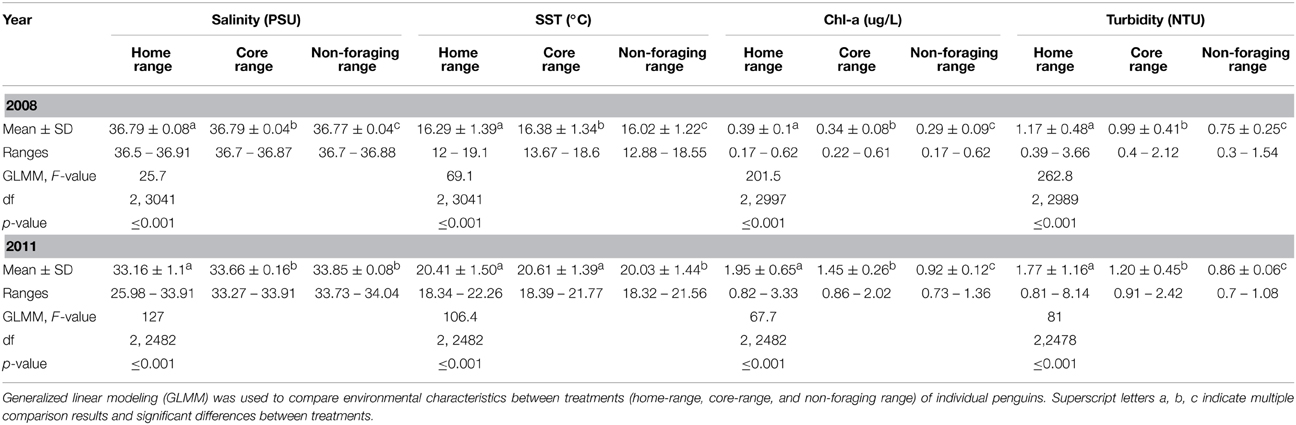
Table 1. Comparison of mean ± SD physico-chemical characteristics measured within the home-range, core-range and non-foraging range of little penguins (Eudyptula minor) in 2008 and 2011.
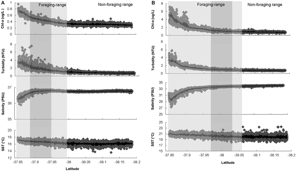
Figure 2. (A) Environmental characteristics measured along the Ship of Opportunity route during the 2008 penguin breeding season (Oct–Jan), commencing at Station Pier, in close proximity to the Yarra River mouth and ending at a latitudinal coordinate of −38.18°S approximately 30 km (straight line distance) from the St Kilda penguin colony. Shaded areas indicate the mean 2008 foraging range of penguins and comprise the home-range (95% KUD) shaded in light gray, and the core-range (50% KUD) shaded in dark gray. The non-shaded area represents the mean 2008 non-foraging range of penguins. (B) Environmental characteristics measured along the Ship of Opportunity route during the 2011 penguin breeding season (Nov–Jan), commencing at Station Pier, in close proximity to the Yarra River mouth and ending at a latitudinal coordinate of −38.18°S approximately 30 km (straight line distance) from the St Kilda penguin colony. Shaded areas indicate the mean 2011 foraging range of penguins and comprise the home-range (95% KUD) shaded in light gray, and the core-range (50% KUD) shaded in dark gray. The non-shaded area represents the mean 2008 non-foraging range of penguins.
In 2008, significant differences between environmental conditions in the home-range compared to those in the core-range were found, where waters in core-ranges contained lower Chl-a biomass (Z = −18.4, P = 0·001) and turbidity (Z = −21.8, P ≤ 0·001). Additionally, waters in the core-range were more saline (Z = −6.9, P ≤ 0·001), and warmer (Z = 2.4, P ≤ 0·05) compared to the home-range.
Environmental Conditions in 2011
Despite inter-annual and seasonal variations in climatic conditions, similar trends in environmental conditions between the foraging range and non-foraging range of penguins were found in 2011 (Table 1). Significant differences in environmental conditions between the foraging and non-foraging range were observed, and environmental conditions in the foraging range were substantially more dynamic than in the non-foraging range (Table 1, Figure 2B). Penguins foraged in waters with higher Chl-a biomass [F(1, 2483) = 36.4, P ≤ 0·001], turbidity [F(1, 2479) = 17.4, P ≤ 0·001], and in waters with higher temperatures [F(1, 2483) = 212.2, P ≤ 0·001] compared to the non-foraging range. However, no difference in salinity between the foraging range and non-foraging range was found [F(1, 2483) = 2.5, P > 0·05]. Environmental conditions within the home-range of penguins contained higher Chl-a biomass (Z = 11.3, P ≤ 0·001) and turbidity (Z = 11.3, P ≤ 0·001), were warmer (Z = 13.8, P = 0·001), and less saline (Z = −12.2, P = 0·001) compared to the non-foraging range. Compared to the non-foraging range, environmental conditions in the core-range of penguins comprised waters of higher Chl-a biomass (Z = 5.1, P ≤ 0·001) and turbidity (Z = 3.8, P ≤ 0·001), and that were warmer (Z = 11.9, P ≤ 0·001). No difference in salinity between the core-range and non-foraging range was found (Z = −1.2, P > 0·05).
In 2011, waters in core-ranges of penguins contained lower Chl-a biomass (Z = 8.6, P ≤ 0·001) and turbidity (Z = 12, P ≤ 0·001), were more saline (Z = −15.9, P ≤ 0·001), but did not differ in temperature (Z = 2.1, P > 0·05) compared to the home-range.
Discussion
Across years, penguin foraging ranges consistently occurred in waters with significantly higher Chl-a, turbidity, temperature and lower salinity than non-foraging ranges. We think that high Chl-a biomass was probably the key determinant of penguin distribution, as Chl-a rich areas are known to aggregate prey and act as important drivers of foraging effort (Weimerskirch et al., 2004; Ainley et al., 2005; Suryan et al., 2012). Within the foraging range, the core-range of penguins occurred in stable waters with lower productivity and lower turbidity than the near-river home-range. This showed the importance of turbidity to penguin foraging as they foraged in a core zone with less turbid waters even though it had a slightly lower Chl-a concentration. We suggest conditions in these core-ranges are more stable and offer a higher degree of prey predictability compared to conditions in the dynamic home-range. Furthermore, penguins may spend a greater proportion of their time in core-ranges as these waters have relatively low turbidity, which may improve the ability of penguins to detect and capture their prey.
Environmental Differences between the Foraging Range and Non-Foraging Range of Penguins
In 2008, the foraging ranges of penguins were located in the northern regions of the bay, in contrast to the north and central distribution of penguins in 2011 and 2012. Kowalczyk et al. (2015a) reported that penguin 2011 and 2012 distribution shifts were in response to increased river runoff, which had a dispersal effect on nutrients, prey, and therefore, penguins. In this study we examined this relationship further and found that despite the observed shifts in penguin foraging distribution between years, the foraging ranges of penguins in 2008 and 2011 consistently occurred in waters with higher Chl-a content, turbidity, SST and lower salinity than their non-foraging ranges. The presence of penguins in productive waters is in line with several studies that found that seabirds forage in areas of elevated levels of primary productivity (Weimerskirch et al., 2004; Ainley et al., 2005; Suryan et al., 2012). Areas with high Chl-a content are associated with sustained primary productivity and are therefore more likely to attract and aggregate planktivores that in turn provide predictable food sources for planktivorous fish and their predators (Grimes and Finucane, 1991; Ressler et al., 2005; Scales et al., 2014).
We cannot conclude that penguins selected their foraging ranges on the basis of productivity alone. Penguins may have utilized their foraging ranges (northern and central regions) in preference to the non-foraging range (southerly regions) due to the close proximity of these waters to their colony. By foraging close to the colony penguins may have been opting to minimize energy expenditure and reduce time spent foraging in pursuit of other fitness-enhancing activities (Buckley and Buckley, 1980). However, fish surveys conducted in the winters of 2008 and 2011 indicated that anchovy (Engraulis australis), the dominant prey species of penguins in 2008 and 2011 (Kowalczyk et al., 2015a), was most abundant in the central and eastern regions of the bay, and scarce in the southern regions of the bay (Parry and Stokie, 2008; Hirst et al., 2011). Hirst et al. (2011) suggested that the high biomass of anchovies in these regions matched with the abundant biomass of phytoplankton and zooplankton that resulted from the delivery of nutrients from the nearby Yarra and Patterson Rivers. Summer egg and larval surveys confirmed anchovies' preferred use of eastern regions, with highest egg and larval densities found in these areas (Acevedo et al., 2009). These findings are in support of Arnott and Mckinnon (1985) who stated that adult anchovy selectively spawn in plankton-rich areas and suggest that penguins were foraging in these regions due to high prey availability as opposed to distance to foraging areas.
The relatively minor temperature and salinity differences between the foraging and non-foraging ranges of penguins are unlikely to be a key factor in influencing anchovy distribution in Port Phillip Bay. A study on the distribution and abundance of anchovy in relation to temperature and salinity in the nearby Gippsland lakes, found that eggs and larvae occurred in waters with temperatures ranging from 14.8°C to 24.2°C, with the main spawning grounds occurring in waters above 18°C (Arnott and Mckinnon, 1985). Additionally, anchovy eggs were found in salinities ranging from 2.3 to 35.5 psu but most spawning activity occurred in waters above 15.8 psu (Arnott and Mckinnon, 1985). These findings show that anchovies can successfully reproduce in wide temperature and salinity ranges. Given that salinities and temperatures in the foraging and non-foraging ranges of penguins were within the preferred spawning conditions of anchovies, it is unlikely these factors were preventing anchovies from spawning in southerly regions of the bay. These findings suggest that productivity is the key driver of anchovy distribution and the high productivity in the northern and eastern regions of the bay presumably attracted anchovies and subsequently penguins to these regions.
Environmental Differences between the Home-Range and Core-Range of Penguins
Within Port Phillip Bay, waters in the northern section of the home-range occur in close proximity to river outlets. These regions are enriched in nutrients and are subsequently highly productive in terms of primary productivity (Lee et al., 2012). Given the high primary productivity in this region we would expect penguins to intensively forage in these productive areas. But, the core-ranges of penguins occurred away from the Yarra River mouth, in waters that were less productive (lower Chl-a) than the home-range (Figure 1A). Although waters in the core-ranges of penguins had lower Chl-a biomass compared to their home-ranges, it is likely these regions were still highly productive in terms of prey availability. This is because the temporal lag between the delivery of nutrients from the Yarra and Patterson rivers, their subsequent transport away from point sources, and eventual uptake and assimilation by phytoplankton, and in-turn, zooplankton, may have led to the spatial displacement of fish from the rivers (Hirst et al., 2011). This spatial displacement of fish may be a key factor driving penguin core-range selection and may explain why the core-ranges of penguins were positioned in waters with comparatively low Chl-a biomass, downstream of the Yarra River (Figure 1A).
Like most seabirds, penguins are visual predators, constrained to forage in daylight (Pelletier et al., 2014) and require minimum light thresholds to locate and capture their prey (Cannell and Cullen, 1998; Ropert-Coudert et al., 2006). Thus, water visibility would be a major factor on habitat selection but few studies have examined the effect of turbidity in foraging preferences of meso-top predators. Here we showed that the core-ranges of penguins occurred in waters that were less turbid compared to the home-range, which is an area subject to much river runoff (Lee et al., 2012). By foraging in relatively productive waters but with low turbidity and therefore higher light levels, penguins may be optimizing their ability to detect and capture prey. Slight increases in turbidity levels potentially have significant effects on their foraging efficiency, particularly in deeper waters where a small increase in turbidity has a large cumulative effect on visibility at depth (Eiane et al., 1999). In addition to reducing ambient light intensity, turbidity scatters light and thereby reduces the apparent difference in brightness between a prey item and its background, a phenomenon known as contrast degradation (Lythgoe, 1979). Therefore, by foraging in waters with low turbidity, penguins likely increase their prey visibility and encounter rate, and reduce the probability that prey will manoeuver their way outside of the penguin's field of view (De Robertis et al., 2003).
Less dynamic waters may also be related to the fish habitat preferences. Waters in the core-ranges of penguins were stable, with a lower range in environmental variables compared to the home-range. Several studies have found that species diversity and fish abundance is lower in dynamic-salinity environments compared to stable-salinity environments, as rapid fluctuations in salinity can present a significant stress for fish species (Serafy et al., 1997). Moreover, for marine spawners, including anchovies, large declines in salinity (salinity levels <15 psu) can be detrimental to successful fertilization and can present unfavorable incubation conditions for eggs (Arnott and Mckinnon, 1985). In Port Phillip Bay, following a heavy rainfall event, Longmore et al. (1999) recorded salinities as low as 5 psu in the Yarra River Mouth, and as low as 15 psu in Hobson Bay, the northern most region of the bay. The dynamic fluctuations in salinity in Hobson Bay may thus deter fish from both residing and spawning in this region and may explain the low biomass of fish in this region in 2008 and 2011 (Hirst et al., 2011). The poor prey availability in Hobson Bay would have a subsequent effect on the foraging distribution of penguins.
Similarly to salinity, temperature plays a dominant role in regulating fish metabolic processes and rapid changes to their specific temperature regimes can have significant effects on their physiology and behavior (Szekeres et al., 2014). Some species are able to habituate to rapid fluctuations in temperature (Tanck et al., 2000), while for others, sudden temperature changes can induce physiological stress that can lead to behavioral impairments (Szekeres et al., 2014). Although penguin prey are tolerant to wide ranges in temperature, exemplified by their within-year and between-year presence in the bay (Parry et al., 2009; Hirst et al., 2010, 2011), it is unclear how they respond to rapid fluctuations in water temperature and whether rapid temperature shifts close to point sources would influence their distribution. Regulating physiological and behavioral impairments is energetically costly and by residing in dynamic environments fish may compromise their growth and reproductive potential (Szekeres et al., 2014). Therefore, we would expect that regions with stable temperatures would provide a more favorable environment for both penguin prey and penguins.
Other factors not addressed in this study could be playing a role in low biomass of fish in Hobson Bay. For highly urbanized embayments like Port Phillip Bay, rapid fluctuations in dissolved oxygen, pollutants and contaminants at point sources have been associated with lower abundance and richness of marine invertebrate and vertebrate (including fish) communities (Petersen and Pihl, 1995; Wu, 2009; Mckinley and Johnston, 2010). However, species abundance and richness at point sources is not consistently lower in urbanized environments and may vary from system to system (Mckinley et al., 2011a,b). Nevertheless, by intensively foraging in waters that are relatively stable in terms of salinity, temperature and turbidity, and in waters that contain relatively high levels of productivity (e.g., Chl-a), penguins may be utilizing areas that offer consistently favorable conditions for prey, thereby having access to a relatively predictable supply of resources.
Finally, the selection of foraging–ranges around shipping channels can also be attributed to the influence of physical features of the shipping channel on penguin foraging efficiency. Preston et al. (2008) observed that the diving shape profiles and foraging locations of penguins corresponded with the locations and physical features (e.g., depth, angle) of the shipping channel and suggested penguins may be using shipping channels to reduce the escape field of prey. However, if penguins are using shipping channels to improve capture success rate then we would expect their foraging trajectories to be linear, similar to the tracks of yellow-eyed penguins (Megadyptes antipodes) in the Otago Peninsula, that travel in straight lines for several kilometers following demersal fish trawl furrows on the seafloor (Mattern et al., 2013), or zigzagged, reflecting the continued use of the shipping channel. Furthermore, if exploiting shipping channels is a means to improve foraging efficiency, we would expect the foraging ranges of a greater proportion of sampled penguins to overlap with the shipping channel. In light of these findings it is likely penguins utilized regions overlapping with shipping channels mainly due to environmental conditions that aggregated prey in these regions rather than as a foraging tactic to improve prey capture rate.
Limitations and Conclusion
The cost of obtaining oceanographic data to combine with biological data in higher trophic-level predator studies are usually prohibitive and therefore rare to obtain. Ships of Opportunity provide valuable environmental data that are very useful to seabird foraging studies. In our study, Ship of Opportunity data were collected on daily transects over the same route, providing a robust oceanographic picture. Despite these benefits, there are some drawbacks. Firstly, penguins/diving seabirds do not follow the exact transects traversed by ships. Consequently, significant parts of home-ranges and core-ranges fall on either side of transects, and it is unclear how environmental conditions in these areas vary from conditions within transects. As such, while we can gain information on environmental conditions within seabird home-and core-ranges, caution should be exercised to not extrapolate these conditions to their entire foraging range. However, because the foraging areas of little penguins are comparatively small, with the peripheries of home- and core-ranges falling within 10 km of the Spirit of Tasmania transect, we considered environmental conditions collected daily along the transect to be indicative of conditions in their foraging–range. Secondly, within dynamic regions such as river plumes, it can be unclear how the physical presence of a large shipping vessel affects measurements of environmental conditions within the sampled area. However, Ship of Opportunity data quality control and validation procedures are usually rigorous and in Port Phillip Bay data collected from the Spirit of Tasmania has been found to closely correlate with SST measured by moored buoys and data obtained from the Advanced Along Track Scanning Radiometer on the EnviSat polar-orbiting satellite (Beggs et al., 2012). Finally, necessary frequent maintenance and calibration of the autonomous sampling systems can lead to missing data. In this study, 11 penguins foraged along the shipping channel in 2012 but due to system maintenance we were unable to correlate environmental conditions with the foraging characteristics of little penguins in 2012, greatly reducing the sample size of this study.
Nevertheless, by coupling data obtained from bio-logging technologies and a Ship of Opportunity, we found that little penguins have close access to, and forage within, productive waters that appear to attract a large variety of prey taxa. Close proximity to abundant resources is of critical importance to the survival and breeding success of this short-ranging, central place forager. Despite their close proximity to productive waters, the breeding performance of little penguins is highly variable and this variability has been attributed to fluctuations in prey abundance and diversity (Kowalczyk et al., 2014). Consequently, the St Kilda penguin colony is vulnerable to changes in prey availability in local waters, particularly during the breeding season when adults are constrained by their need to feed chicks regularly (Chiaradia and Nisbet, 2006). Studies aimed at investigating how biotic and abiotic factors in plume fronts influence fish recruitment and distribution will be important to managing the resources that inshore seabirds depend upon.
Author Contributions
Conceived and designed the experiments: NK, AC, TP, and RR. Performed the experiments: NK and TP. Processed data: NK, TP. Analyzed the data: NK. Wrote the paper: NK, AC, TP, RR. Final approval of the manuscript: NK, AC, TP, RR.
Conflict of Interest Statement
The authors declare that the research was conducted in the absence of any commercial or financial relationships that could be construed as a potential conflict of interest.
Acknowledgments
Parks Victoria granted permission to work along the breakwater. We thank Holsworth Wildlife Research Trust and Coastcare Australia for financial support. We acknowledge Earthcare St Kilda and Phillip Island Nature Parks for their continued support to little penguin research at St Kilda. We thank all research volunteers for their field assistance, Christopher Johnstone for statistical advice, Bronwyn Isaac who assisted with the map design, and Annett Finger who improved earlier drafts of this manuscript.
References
Acevedo, S., Jenkins, G. P., and Kent, J. (2009). Baywide Egg and Larval Surveys Sub-program. Milestone report No. 3, in Technical Report Series No. 65, Department of Primary Industries, Queenscliff, VIC.
Adams, J., Takekawa, J. Y., Carter, H. R., and Yee, J. (2010). Factors influencing the at-sea distribution of Cassin's Auklets (Ptychoramphus aleuticus) that breed in the Channel Islands, California. The Auk 127, 503–513. doi: 10.1525/auk.2010.09273
Ainley, D. G., Spear, L. B., Tynan, C. T., Barth, J. A., Pierce, S. D., Glenn Ford, R., et al. (2005). Physical and biological variables affecting seabird distributions during the upwelling season of the northern California Current. Deep Sea Res. II Top. Stud. Oceanogr. 52, 123–143. doi: 10.1016/j.dsr2.2004.08.016
Arnott, G., and Mckinnon, A. (1985). Distribution and abundance of eggs of the anchovy, Engraulis australis antipodum Gunther, in relation to temperature and salinity in the Gippsland Lakes. Marine Freshw. Res. 36, 433–439. doi: 10.1071/MF9850433
Beggs, H., Verein, R., Paltoglou, G., Kippo, H., and Underwood, M. (2012). Enhancing ship of opportunity sea surface temperature observations in the Australian region. J. Oper. Oceanogr. 5, 59–73. doi: 10.1080/1755876X.2012.11020132
Buckley, F., and Buckley, P. (1980). “Habitat selection and marine birds,” in Behavior of Marine Animals, eds J. Burger, B. Olla, and H. Winn (New York, NY: Springer), 69–112.
Calenge, C. (2006). The package “adehabitat” for the R software: a tool for the analysis of space and habitat use by animals. Ecol. Model. 197, 516–519. doi: 10.1016/j.ecolmodel.2006.03.017
Cannell, B. L., and Cullen, J. M. (1998). The foraging behaviour of Little Penguins Eudyptula minor at different light levels. Ibis 140, 467–471. doi: 10.1111/j.1474-919X.1998.tb04608.x
Chiaradia, A., and Nisbet, I. C. T. (2006). Plasticity in parental provisioning and chick growth in little penguins Eudyptula minor in years of high and low breeding success. Ardea 94, 257–270.
Collins, M., Cullen, J. M., and Dann, P. (1999). Seasonal and annual foraging movements of little penguins from Phillip Island, Victoria. Wildl. Res. 26, 705–721. doi: 10.1071/WR98003
Commins, M. L., Ansorge, I., and Ryan, P. G. (2014). Multi-scale factors influencing seabird assemblages in the African sector of the Southern Ocean. Antarct. Sci. 26, 38–48. doi: 10.1017/S0954102013000138
De Robertis, A., Ryer, C. H., Veloza, A., and Brodeur, R. D. (2003). Differential effects of turbidity on prey consumption of piscivorous and planktivorous fish. Can. J. Fish. Aquat. Sci. 60, 1517–1526. doi: 10.1139/f03-123
Eiane, K., Aksnes, D. L., Bagoien, E., and Kaartvedt, S. (1999). Fish or jellies—a question of visibility? Limnol. Oceanogr. 44, 1352–1357. doi: 10.4319/lo.1999.44.5.1352
Evans, K., Brown, J. N., Sen Gupta, A., Nicol, S. J., Hoyle, S., Matear, R., et al. (2014). When 1+1 can be >2: Uncertainties compound when simulating climate, fisheries and marine ecosystems. Deep Sea Res. II Topic. Stud. Oceanogr. 113, 312–322. doi: 10.1016/j.dsr2.2014.04.006
Ford, R. G., and Krumme, D. W. (1979). The analysis of space use patterns. J. Theor. Biol. 76, 125–155. doi: 10.1016/0022-5193(79)90366-7
Grimes, C. B., and Finucane, J. H. (1991). Spatial distribution and abundance of larval and juvenile fish, chlorophyll and macrozooplankton around the Mississippi River discharge plume, and the role of the plume in fish recruitment. Marine Ecol. Progr. Ser. 75, 109–119. doi: 10.3354/meps075109
Grimes, C., and Kingsford, M. (1996). How do riverine plumes of different sizes influence fish larvae: do they enhance recruitment? Marine Freshw. Res. 47, 191–208. doi: 10.1071/MF9960191
Harris, G. (1996). Port Phillip Bay Environmental Study: Final Report. Melbourne, VIC: CSIRO Publishing.
Hirst, A. J., White, C. A., Green, C., Werner, G. F., Heislers, S., and Spooner, D. (2011). Baywide Anchovy Study Sub-Program. Milestone report No. 4. Technical report No. 150, Department of Primary Industries, Queenscliff, VIC.
Hirst, A. J., White, C. A., Heislers, S., Werner, G. F., and Spooner, D. (2010). Baywide Anchovy Study Sub-Program. Milestone report no. 3, Technical Report No. 114. Department of Primary Industries, Queenscliff, VIC.
Joint, I., and Groom, S. B. (2000). Estimation of phytoplankton production from space: current status and future potential of satellite remote sensing. J. Exp. Mar. Biol. Ecol. 250, 233–255. doi: 10.1016/S0022-0981(00)00199-4
Joiris, C., Humphries, G. W., and De Broyer, A. (2013). Seabirds encountered along return transects between South Africa and Antarctica in summer in relation to hydrological features. Polar Biol. 36, 1633–1647. doi: 10.1007/s00300-013-1382-9
Kaufman, J. H. (1962). Ecology and social behaviour of the coati Nasua nirica on Barro Colorado island, Panama. Univ. Calif. Publ. Zool. 95–222.
Kowalczyk, N. D., Chiaradia, A., Preston, T. J., and Reina, R. D. (2014). Linking dietary shifts and reproductive failure in seabirds: a stable isotope approach. Funct. Ecol. 28, 755–765. doi: 10.1111/1365-2435.12216
Kowalczyk, N. D., Chiaradia, A., Preston, T. J., and Reina, R. D. (2015a). Environmental variability drives shifts in the foraging behaviour and reproductive success of an inshore seabird. Oecologia. doi: 10.1007/s00442-015-3294-6. [Epub ahead of print].
Kowalczyk, N. D., Chiaradia, A., Preston, T. J., and Reina, R. D. (2015b). Fine-scale dietary changes between the breeding and non-breeding diet of a resident seabird. R. Soc. Open Sci. 2:140291. doi: 10.1098/rsos.140291
Le Fèvre, J. (1987). “Aspects of the Biology of Frontal Systems,” in Advances in Marine Biology, eds J. H. S. Blaxter and A. J. Southward (New York, NY: Academic Press), 163–299.
Lee, R., Black, K., Bosserel, C., and Greer, D. (2012). Present and future prolonged drought impacts on a large temperate embayment: Port Phillip Bay, Australia. Ocean Dyn. 62, 907–922. doi: 10.1007/s10236-012-0538-4
Lee, R. S., Mancini, S., Martinez, G., and Lindsay, M. (2011). “Resolving environmental dynamics in Port Phillip Bay, using high repeat sampling off the Spirit of Tasmania 1,” in Coasts and Ports 2011: Diverse and Developing: Proceedings of the 20th Australasian Coastal and Ocean Engineering Conference and the 13th Australasian Port and Harbour Conference (Barton, MI).
Longmore, A., Heggie, D., Flint, R., Cowdell, R., and Skyring, G. (1999). Impact of runoff on nutrient patterns in northern Port Phillip Bay, Victoria. J. Aust. Geol. Geophys. 17, 203–210.
Mattern, T., Ellenberg, U., Houston, D. M., Lamare, M., Davis, L. S., Van Heezik, Y., et al. (2013). Straight line foraging in yellow-eyed penguins: new insights into cascading fisheries effects and orientation capabilities of marine predators. PLoS ONE 8:e84381. doi: 10.1371/journal.pone.0084381
Mckinley, A. C., Dafforn, K. A., Taylor, M. D., and Johnston, E. L. (2011a). High levels of sediment contamination have little influence on estuarine beach fish communities. PLoS ONE 6:e26353. doi: 10.1371/journal.pone.0026353
Mckinley, A. C., Miskiewicz, A., Taylor, M. D., and Johnston, E. L. (2011b). Strong links between metal contamination, habitat modification and estuarine larval fish distributions. Environ. Pollut. 159, 1499–1509. doi: 10.1016/j.envpol.2011.03.008
Mckinley, A., and Johnston, E. L. (2010). Impacts of contaminant sources on marine fish abundance and species richness: a review and meta-analysis of evidence from the field. Mar. Ecol. Prog. Ser. 420, 175–191. doi: 10.3354/meps08856
Parry, G. D., Stokie, T., Hirst, A. J., Green, C., White, C. A., Heislers, S., et al. (2009). Baywide Anchovy Study Sub-Program. Milestone report No. 2, Technical Report No. 73. Department of Primary Industries, Queenscliff, VIC.
Parry, G., and Stokie, T. (2008). Baywide Anchovy Study Sub-Program. Milestone report No.1 Technical Report No. 23. Department of Primary Industries, Queenscliff, VIC.
Pelletier, L., Chiaradia, A., Kato, A., and Ropert-Coudert, Y. (2014). Fine-scale spatial age segregation in the limited foraging area of an inshore seabird species, the little penguin. Oecologia 176, 399–408. doi: 10.1007/s00442-014-3018-3
Petersen, J., and Pihl, L. (1995). Responses to hypoxia of plaice, Pleuronectes platessa, and dab, Limanda limanda, in the south-east Kattegat: distribution and growth. Environ. Biol. Fishes 43, 311–321. doi: 10.1007/BF00005864
Petersen, W., Schroeder, F., and Bockelmann, F.-D. (2011). FerryBox - Application of continuous water quality observations along transects in the North Sea. Ocean Dynamics 61, 1541–1554. doi: 10.1007/s10236-011-0445-0
Pinheiro, J., Bates, D., Debroy, S., Sarkar, D., and Team, R. C. (2013). Linear and Nonlinear Mixed Effects Models. R Package Version 3.1–108. Avaliable online at: http://cran.r-project.org/web/packages/nlme/index.html
Port of Melbourne. (2013). Port of Melbourne Corporation Operations Handbook Harbour Master's Directions. Melbourne, VIC.
Preston, T. (2010). Relationships Between Foraging Behaviour, Diet and Reproductive Success at an Urban Colony of Little Penguins (Eudyptula minor). Doctoral Thesis, Monash University, St Kilda, VIC.
Preston, T. J., Chiaradia, A., Caarels, S. A., and Reina, R. D. (2010). Fine-scale biologging of an inshore marine animal. J. Exp. Mar. Biol. Ecol. 390, 196–202. doi: 10.1016/j.jembe.2010.04.034
Preston, T., Ropert-Coudert, Y., Kato, A., Chiaradia, A., Kirkwood, R., Dann, P., et al. (2008). Foraging behaviour of little penguins Eudyptula minor in an artificially modified environment. Endanger. Species Res. 4, 95–103. doi: 10.3354/esr00069
R Core Development Team. (2013). “R: a language and environment for statistical computing,” in R Foundation for Statistical Computing (Vienna).
Ressler, P. H., Brodeur, R. D., Peterson, W. T., Pierce, S. D., Mitchell Vance, P., Røstad, A., et al. (2005). The spatial distribution of euphausiid aggregations in the Northern California Current during August 2000. Deep Sea Res, II Topic. Stud. Oceanogr. 52, 89–108. doi: 10.1016/j.dsr2.2004.09.032
Ropert-Coudert, Y., Kato, A., Wilson, R., and Cannell, B. (2006). Foraging strategies and prey encounter rate of free-ranging Little Penguins. Mar. Biol. 149, 139–148. doi: 10.1007/s00227-005-0188-x
Ropert-Coudert, Y., Knott, N., Chiaradia, A., and Kato, A. (2007). How do different data logger sizes and attachment positions affect the diving behaviour of little penguins? Deep Sea Res. II Topic. Stud. Oceanogr. 54, 415–423. doi: 10.1016/j.dsr2.2006.11.018
Sampson, J., Easton, A., and Singh, M. (2014). “Port phillip bay,” in Estuaries of Australia in 2050 and Beyond, ed E. Wolanski (Dordrecht: Springer), 49–68.
Scales, K. L., Miller, P. I., Embling, C. B., Ingram, S. N., Pirotta, E., and Votier, S. C. (2014). Mesoscale fronts as foraging habitats: composite front mapping reveals oceanographic drivers of habitat use for a pelagic seabird. J. R. Soc. Interface 11, 20140679–20140679. doi: 10.1098/rsif.2014.0679
Serafy, J. E., Lindeman, K. C., Hopkins, T. E., and Ault, J. S. (1997). Effects of freshwater canal discharge on fish assemblages in a subtropical bay: field and laboratory observations. Mar. Ecol. Prog. Ser. 160, 161–172. doi: 10.3354/meps160161
Shaffer, S., Tremblay, Y., Awkerman, J., Henry, R. W., Teo, S. H., Anderson, D., et al. (2005). Comparison of light- and SST-based geolocation with satellite telemetry in free-ranging albatrosses. Mar. Biol. 147, 833–843. doi: 10.1007/s00227-005-1631-8
Skov, H., and Prins, E. (2001). Impact of estuarine fronts on the dispersal of piscivorous birds in the German Bight. Mar. Ecol. Prog. Ser. 214, 279–287. doi: 10.3354/meps214279
Suryan, R. M., Santora, J. A., and Sydeman, W. J. (2012). New approach for using remotely sensed chlorophyll a to identify seabird hotspots. Mar. Ecol. Prog. Ser. 451, 213–225. doi: 10.3354/meps09597
Szekeres, P., Brownscombe, J. W., Cull, F., Danylchuk, A. J., Shultz, A. D., Suski, C. D., et al. (2014). Physiological and behavioural consequences of cold shock on bonefish (Albula vulpes) in The Bahamas. J. Exp. Mar. Biol. Ecol. 459, 1–7. doi: 10.1016/j.jembe.2014.05.003
Tanck, M. W. T., Booms, G. H. R., Eding, E. H., Bonga, S. E. W., and Komen, J. (2000). Cold shocks: a stressor for common carp. J. Fish Biol. 57, 881–894. doi: 10.1111/j.1095-8649.2000.tb02199.x
Tremblay, Y., Bertrand, S., Henry, R. W., Kappes, M. A., Costa, D. P., and Shaffer, S. A. (2009). Analytical approaches to investigating seabird–environment interactions: a review. Mar. Ecol. Prog. Ser. 391, 153–163. doi: 10.3354/meps08146
Wagner, C. M., and Austin, H. M. (1999). Correspondence between environmental gradients and summer littoral fish assemblages in low salinity reaches of the Chesapeake Bay, USA. Marine Ecol. Prog. Ser. 177, 197–212. doi: 10.3354/meps177197
Wakefield, E. D., Phillips, R. A., and Matthiopoulos, J. (2009). Quantifying habitat use and preferences of pelagic seabirds using individual movement data: a review. Mar. Ecol. Prog. Ser. 391, 165–182. doi: 10.3354/meps08203
Weimerskirch, H., Corre, M. L., Jaquemet, S. B., Potier, M., and Marsac, F. (2004). Foraging strategy of a top predator in tropical waters: great frigatebirds in the Mozambique Channel. Mar. Ecol. Prog. Ser. 275, 297–308. doi: 10.3354/meps275297
Wilson, R. P., Pütz, K., Peters, G., Culik, B., Scolaro, J. A., Charrassin, J.-B., et al. (1997). Long-term attachment of transmitting and recording devices to penguins and other seabirds. Wildl. Soc. Bull. 25, 101–106.
Wu, R. S. S. (2009). Effects of hypoxia on fish reproduction and development. Fish Physiol. 27, 79–141. doi: 10.1016/S1546-5098(08)00003-4
Keywords: penguin, anchovy, river front, Ship of Opportunity, core-range, home-range
Citation: Kowalczyk ND, Reina RD, Preston TJ and Chiaradia A (2015) Selective foraging within estuarine plume fronts by an inshore resident seabird. Front. Mar. Sci. 2:42. doi: 10.3389/fmars.2015.00042
Received: 09 March 2015; Accepted: 29 May 2015;
Published: 16 June 2015.
Edited by:
Jesper H. Andersen, NIVA Denmark Water Research, DenmarkReviewed by:
Ricardo Serrão Santos, University of the Azores, PortugalKatherine Dafforn, University of New South Wales, Australia
Copyright © 2015 Kowalczyk, Reina, Preston and Chiaradia. This is an open-access article distributed under the terms of the Creative Commons Attribution License (CC BY). The use, distribution or reproduction in other forums is permitted, provided the original author(s) or licensor are credited and that the original publication in this journal is cited, in accordance with accepted academic practice. No use, distribution or reproduction is permitted which does not comply with these terms.
*Correspondence: Richard D. Reina, School of Biological Sciences, 25 Rainforest Walk, Monash University, Clayton, VIC 3800, Australia, richard.reina@monash.edu