


Abstract
We have selected the positions of 54 6.7 GHz methanol masers from the Methanol Multibeam Survey catalogue, covering a range of longitudes between 20° and 34° of the Galactic plane. These positions were mapped in the J = 3-2 transition of both the 13CO and C18O lines. A total of 58 13CO emission peaks are found in the vicinity of these maser positions. We search for outflows around all 13CO peaks, and find evidence for high-velocity gas in all cases, spatially resolving the red and blue outflow lobes in 55 cases. Of these sources, 44 have resolved kinematic distances, and are closely associated with the 6.7 GHz masers, a subset referred to as Methanol Maser Associated Outflows (MMAOs). We calculate the masses of the clumps associated with each peak using 870 μm continuum emission from the ATLASGAL survey. A strong correlation is seen between the clump mass and both outflow mass and mechanical force, lending support to models in which accretion is strongly linked to outflow. We find that the scaling law between outflow activity and clump masses observed for low-mass objects, is also followed by the MMAOs in this study, indicating a commonality in the formation processes of low-mass and high-mass stars.
INTRODUCTION
Massive stars (>8 M⊙) play a key role in the evolution of the Universe, as the principal sources of heavy elements and UV radiation. Their winds, massive outflows, expanding H ii regions and supernova explosions serve as an important source of enrichment, mixing and turbulence in the interstellar medium (ISM) of galaxies (Zinnecker & Yorke 2007). Our understanding of the formation and evolution of young massive stars is made difficult by their rarity, large average distances that demands observations at higher angular resolution, deeply embedded formation within dense clusters resulting in confusing dynamics and obscuration, and rapid evolution with short-lived evolutionary phases (Shepherd & Churchwell 1996b; Zinnecker & Yorke 2007).
The specific formation process of massive stars is not yet fully understood. These stars reach the zero-age main sequence while still accreting material from their parent molecular cloud. Due to their high mass, they radiate strongly. This radiation pressure exceeds the gravitational pressure, and should the formation process be similar to low-mass stars, the growing radiation pressure from the newborn stars will eventually become strong enough to stop the accretion, yielding an upper mass limit of ∼40 M⊙ (Wolfire & Cassinelli 1987; Stahler & Palla 1993).
Previously, two solutions were proposed to overcome this problem: (i) a formation process involving multiple lower mass stars, either via coalescence of low- to intermediate-mass protostars (e.g. Bonnell, Bate & Zinnecker 1998; Bally & Zinnecker 2005), or competitive accretion in a clustered environment (e.g. Bonnell, Vine & Bate 2004), or (ii) a scaled-up version of the process found in low-mass star formation. The latter solution can be subdivided into the following main categories: (a) increased spherical accretion rates in turbulent cloud cores (order 10−4–10−3 M⊙ yr−1), high enough to overcome the star's radiation pressure (e.g. Norberg & Maeder 2000; McKee & Tan 2003) or (b) accretion via discs on to a single massive star (e.g. Jijina & Adams 1996; Yorke & Sonnhalter 2002).
A solution to overcome the radiation pressure barrier was proposed by Yorke & Sonnhalter (2002), that involved the generation of a strong anisotropic radiation field where an accretion disc reduces the effects of radiative pressure, by allowing photons to escape along the polar axis (the ‘flashlight effect’). However, these simulations showed an early end of the disc accretion phase, with final masses limited to ∼42 M⊙. Krumholz et al. (2009) suggested that the early end of the accretion phase is because the disc loses its shielding property as it cannot be fed in an axially symmetric configuration. Contrary to the stable radiation pressure-driven outflows in Yorke & Sonnhalter (2002), they proposed a three-dimensional radiation hydrodynamic simulation with a Rayleigh–Taylor instability in the outflow region, allowing further accretion on to the disc.
Kuiper et al. (2010) took this further by introducing a dust sublimation front to their simulations. This preserves the shielding of the massive accretion disc and allows the protostar to grow to ∼140 M⊙.
The easiest way to verify the disc accretion models, would be with the detection of accretion discs around massive protostars, but this is difficult without specialized techniques (e.g. Pestalozzi, Elitzur & Conway 2009), because they are small (at most several hundred au), short lived, and easily confused by envelopes (Kim & Kurtz 2006). Few clear examples of such discs exist (e.g. Cesaroni et al. 2007; Zapata, Tang & Leurini 2010).
However, we expect that if massive stars do form via accretion discs, they will generate massive and powerful outflows, similar to low-mass stars. These outflows are necessary to transport angular momentum away from a forming star (Shu et al. 1991, 2000; Konigl & Pudritz 2000; Chrysostomou et al. 2008). For massive stars, these outflows should be of much larger scale and easier to detect than the accretion discs (Kim & Kurtz 2006). Studying outflows offers an alternative approach to probe the embedded core.
There have been many studies that collectively suggest outflows are ubiquitously associated with massive star formation (e.g. Shepherd & Churchwell 1996a; Molinari et al. 1998; Beuther et al. 2002b; Xu et al. 2006).
Zhang et al. (2005) found outflow masses (∼tens to hundreds M⊙), momenta (10–100 M⊙ km s−1) and energies (∼1039 J) towards their sample of luminous IRAS point sources about a factor 10 higher than the values of low-mass outflows (Bontemps et al. 1996). This suggests that outflows consist of accelerated gas that has been driven by a young accreting protostar, rather than swept-up ambient material (Churchwell 1999). It could also be material that originates from the accretion disc/young stellar object (YSO) and is funnelled out of the central system (e.g. Shepherd & Churchwell 1996a).
To date, CO observations of molecular outflows have been made using mainly two methods: (1) single-point CO line surveys towards samples of massive YSOs in search of high-velocity (HV) molecular gas (e.g. Shepherd & Churchwell 1996b; Sridharan et al. 2002) or (2) CO line mapping of carefully selected sources that exhibit HV wings (e.g. Shepherd & Churchwell 1996a; Beuther et al. 2002b). Unless outflows are mapped, it is difficult to determine their physical properties. Mapping outflows at sufficient sensitivity and high angular resolution is time-consuming, but the development of heterodyne focal plane arrays [e.g. HARP on James Clerk Maxwell Telescope (JCMT) or HERA on Institut de Radioastronomie Millimétrique (IRAM)] has made it possible to map statistically significant samples of massive star-forming regions to search for outflows l(e.g. López-Sepulcre et al. 2009; Gottschalk et al. 2012).
Outflows are one of the earliest observable signatures of star formation, and are believed to develop from the central objects during the infrared bright stage called the ‘hot core’ phase (Cesaroni, Walmsley & Churchwell 1992; Kurtz et al. 2000), just before the UCHii phase (Shepherd & Churchwell 1996a; Wu et al. 1999; Zhang et al. 2001; Beuther et al. 2002b; Molinari et al. 2002).
Another important signpost of the ‘hot core’ phase is the turn-on of radiatively pumped 6.7 GHz (class II) methanol masers, the second brightest masers in the Galaxy (Menten 1991; Sobolev, Cragg & Godfrey 1997; Minier et al. 2003). Observations indicate that these masers are rarely associated with H ii regions, but most of them are found to be associated with massive millimetre and submillimetre sources (e.g. Beuther et al. 2002b; Walsh et al. 2003; Urquhart et al. 2013a). It appears as if these masers occupy a brief phase in the pre-UCHii region, even as short as ∼104 yr, and disappear as the UCHii region evolves (Hatchell et al. 1998; Codella & Moscadelli 2000; Codella et al. 2004; van der Walt 2005; Wu et al. 2010). They are also known to be mostly associated with massive star formation, making them important signposts of massive star formation (Minier et al. 2005; Ellingsen 2006; Breen et al. 2013; Caswell 2013).
However, there are limited simultaneous studies of methanol masers and outflow activity. Minier, Conway & Booth (2001) found that 10 out of 13 absolute positions for class II methanol maser sites coincided with typical tracers of massive star formation (e.g. UCHii regions, outflows and hot cores), while seven out of these ten were within less than 2000 au (∼10−2 pc) from outflows. Their results supported the expected association between the occurrence of class II methanol masers and molecular outflows.
The Spitzer GLIMPSE survey (Churchwell et al. 2009) revealed a new signpost for outflows in high-mass star formation regions in the form of extended emission which is bright in the 4.5-μm band. These objects are generally referred to either as extended green objects (EGOs; Cyganowski et al. 2008) or green fuzzies (Chambers et al. 2009). The enhanced emission in this wavelength range is believed to be due to shock-excited H2 and/or CO band-head emission (De Buizer & Vacca 2010). Cyganowski et al. (2008) found that many EGOs are associated with 6.7 GHz methanol masers, while Chen, Ellingsen & Shen (2009) showed a high rate of association with shock-excited class I methanol masers at 44 and 95 GHz. Sensitive, high-resolution searches for class II methanol masers towards a small sample of EGOs achieved a detection rates of 64 per cent (although this should be considered an upper limit since most targets had known 6.7 GHz methanol masers in their vicinity), with approximately 90 per cent of these sources also having associated 44 GHz class I methanol maser emission (Cyganowski et al. 2009). These results demonstrate a close association between methanol masers and young high-mass stars with active outflows.
Molecular outflows are more visible than the YSO or its disc, and because of the association of 6.7 GHz methanol masers with massive star formation, searching for outflows towards these masers and studying their physical properties can reveal information regarding the obscured massive cores they are associated with. Moreover, by selecting outflows that are only associated with methanol masers, deliberately biases the resulting sample towards a narrower, relatively well-defined evolutionary range which allows constraints to be placed on the ‘switch-on’ of the outflows and the study of their temporal development. In this paper, we focus on the study of the physical properties of the outflows and the relationship of these properties with those of their embedding clumps. In a following publication (de Villiers et al., in preparation), we will explore the effects of the maser selection bias in our sample and the resulting behaviour in the dynamical ages of our maser selected sample.
We present a survey of 13CO(J = 3-2) outflows towards a sample of 6.7 GHz Methanol Multibeam (MMB) masers (Green et al. 2009; Breen et al. in preparation) using the HARP (Heterodyne Array Receiver Programme) instrument on the JCMT. Observations and data reduction are described in Section 2. In Section 3, we describe the extraction and analysis of the spectra, as well as outflow mapping and outflow detection frequency. The results are presented in Section 4, where we demonstrate the calculation of the outflows’ physical properties and associated clump masses. The relation between the outflow and associated clump properties are examined, and compared with some low-mass relations found in the literature. We also inspect the correlation between outflow and 6.7 GHz maser luminosities, as well as between maser luminosity and clump masses, as a probe of the relationship between the physical properties of the driving force, outflow and associated maser. The main results are summarized in Section 6.
Although the study of the properties of massive molecular outflows and their relation with associated clump masses is not novel per se, the selection of the sources in this study is unique in terms of association with 6.7 GHz masers. This allows the selection of sources within a relatively well-defined evolutionary phase, which potentially could limit the scatter in parameter space compared to previous work. In this paper, we discuss and investigate the physical properties of the Methanol Maser Associated Outflows (MMAOs), and put them in context with other studies. In a second forthcoming paper, we discuss the effect and implications of the 6.7 GHz maser bias of our sample on our results.
OBSERVATIONS AND DATA REDUCTION
A sample of 6.7 GHz methanol masers were drawn from a preliminary catalogue of Northern hemisphere masers from the MMB Survey which has subarcsec positional accuracies (Green et al. 2009). The properties of these masers are described fully in Breen et al. (in preparation). The initial sample selection was chosen to have an even spread in maser luminosity, distance, association with UCHii regions and IR sources. A sample of 70 sources were observed between 20° < l < 34°.
The targets were observed with the JCMT, on the summit of Mauna Kea, Hawaii on seven nights between 2007 May 17 and 2008 July 22. Targets were mapped in the 13CO and C18O(J = 3-2) transitions (330.6 and 329.3 GHz), using the 16-receptor HARP. Only 14 of the 16 receptors were operational at the time of observation. The receptors are laid out in a 4 × 4 grid separated by 30 arcsec and the beam size of the individual receptors at 345 GHz is 14 arcsec. All the data were corrected for a main-beam efficiency of ηmb = 0.66 (Smith et al. 2008; Buckle et al. 2009). A HARP jiggle map (Buckle et al. 2009) produces a fully sampled, 16-point rectangular map with a pixel scale of 6 arcsec and a spectral resolution of 0.06 km s−1. The field of view is approximately 2 arcmin × 2 arcmin. As the typical distance to the methanol maser target sources is >2kpc, and with an estimated maser lifetime of 2.5-4 × 10⁴ yr (van der Walt 2005), the expected outflows from the maser-associated YSOs should be sampled in a single JCMT HARP jiggle-map. The pointing accuracy of the JCMT is of order 2 arcsec or better. Pointing checks were carried out regularly during observation runs to ensure and maintain accuracy.
The weather during the observations was mostly in JCMT-defined band 3, which implies a sky zenith opacity τ225 varying between 0.08 and 0.12 at 225 GHz as measured by the Caltech Submillimeter Observatory tipping radiometer.1
Out of the 70 observed maser coordinates, 16 observations did not meet one or more of the quality thresholds due to (a) too low signal-to-noise (less than ∼2), (b) non-functioning receptors (report unreliable temperatures), or (c) target positioning too close to the field-of-view border or a dead receptor. The remaining 54 target coordinates are listed in Table 1 and occur in the shaded area in Fig. 1.
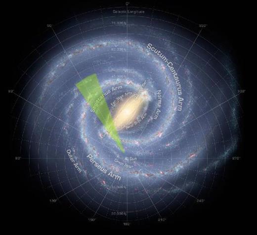
The shaded triangle indicates the approximate area from where the 6.7 GHz methanol maser sample were selected for this study. The background sketch is by R. Hurt and R. Benjamin (Churchwell et al. 2009), and shows how the Galaxy is likely to appear face-on, based on radio, infrared and optical data.
Complete list of 6.7 GHz methanol maser coordinates used as pointing targets, including target names. Suffixes ‘A’ and ‘B’ indicate separate clumps if more than one are detected. The clump coordinates from where spectra were extracted are listed. Sources marked with * had their spectra extracted at the maser coordinate itself. The last column lists the noise rms, integrated over the number of channels nchan in each C18O integrated map (|$\phi = \sigma _{{\rm {{\rm rms}}}} \Delta v \sqrt{n_{{\rm chan}}}$|, for a channel width Δv of 0.5 km s−1). When clumps were truncated at the edge of a map, or signal-to-noise was too low for significant C18O detection, it is indicated.
| Target name | Maser coord. | Clump coord. | ϕ | ||
|---|---|---|---|---|---|
| l(°) | b(°) | l(°) | b(°) | (K km s−1) | |
| G 20.081−0.135 | 20.081 | −0.135 | 20.081 | −0.135 | 1.1 |
| G 21.882+0.013 | 21.882 | 0.013 | 21.875 | 0.008 | 0.9 |
| G 22.038+0.222 | 22.038 | 0.222 | 22.040 | 0.223 | 1.7 |
| G 22.356+0.066 | 22.356 | 0.066 | 22.356 | 0.068 | 2.0 |
| G 22.435−0.169 | 22.435 | −0.169 | 22.435 | −0.169 | 1.3 |
| G 23.003+0.124 | 23.003 | 0.124 | 23.002 | 0.126 | 1.1 |
| G 23.010−0.411 | 23.010 | −0.411 | 23.008 | −0.410 | 2.0 |
| G 23.206−0.378 | 23.206 | −0.378 | 23.209 | −0.378 | 1.0 |
| G 23.365−0.291 | 23.365 | −0.291 | 23.364 | −0.291 | 1.1 |
| G 23.437−0.184 | 23.437 | −0.184 | 23.436 | −0.183 | 1.4 |
| G 23.484+0.097 | 23.484 | 0.097 | 23.483 | 0.098 | 0.9 |
| G 23.706−0.198 | 23.706 | −0.198 | 23.706 | −0.197 | 1.3 |
| G 24.329+0.144 | 24.329 | 0.144 | 24.330 | 0.145 | 1.4 |
| G 24.493−0.039 | 24.493 | −0.039 | 24.493 | −0.039 | 1.4 |
| G 24.790+0.083A | 24.790 | 0.083 | 24.790 | 0.083 | 1.6 |
| G 24.790+0.083B | 24.790 | 0.083 | 24.799 | 0.097 | Cut-off |
| G 24.850+0.087 | 24.850 | 0.087 | 24.853 | 0.085 | 0.9 |
| G 25.650+1.050 | 25.650 | 1.050 | 25.649 | 1.051 | 1.2 |
| G 25.710+0.044 | 25.710 | 0.044 | 25.719 | 0.051 | 1.0 |
| G 25.826−0.178 | 25.826 | −0.178 | 25.824 | −0.179 | 1.2 |
| G 28.148−0.004 | 28.148 | −0.004 | 28.148 | −0.004 | 0.8 |
| G 28.201−0.049 | 28.201 | −0.049 | 28.201 | −0.049 | 1.0 |
| G 28.282−0.359 | 28.282 | −0.359 | 28.289 | −0.365 | 0.6 |
| G 28.305−0.387 | 28.305 | −0.387 | 28.307 | −0.387 | 0.8 |
| G 28.321−0.011 | 28.321 | −0.011 | 28.321 | −0.011 | 0.8 |
| G 28.608+0.018 | 28.608 | 0.018 | 28.608 | 0.018 | 0.7 |
| G 28.832−0.253 | 28.832 | −0.253 | 28.832 | −0.253 | 1.3 |
| G 29.603−0.625 | 29.603 | −0.625 | 29.600 | −0.618 | 1.1 |
| G 29.865−0.043 | 29.865 | −0.043 | 29.863 | −0.045 | 1.6 |
| G 29.956−0.016A | 29.956 | −0.016 | 29.956 | −0.017 | 1.6 |
| G 29.956−0.016B | 29.956 | −0.016 | 29.962 | −0.008 | 1.6 |
| G 29.979−0.047 | 29.979 | −0.047 | 29.979 | −0.048 | 1.7 |
| G 30.317+0.070* | 30.317 | 0.070 | 30.317 | 0.070 | 1.0 |
| G 30.370+0.482A | 30.370 | 0.482 | 30.370 | 0.484 | 0.6 |
| G 30.370+0.482B | 30.370 | 0.482 | 30.357 | 0.487 | Low S/N |
| G 30.400−0.296 | 30.400 | −0.296 | 30.403 | −0.296 | 0.8 |
| G 30.419−0.232 | 30.419 | −0.232 | 30.420 | −0.233 | 1.1 |
| G 30.424+0.466 | 30.424 | 0.466 | 30.424 | 0.464 | 0.5 |
| G 30.704−0.068 | 30.704 | −0.068 | 30.701 | −0.067 | 1.2 |
| G 30.781+0.231 | 30.781 | 0.231 | 30.780 | 0.231 | 1.2 |
| G 30.788+0.204 | 30.788 | 0.204 | 30.789 | 0.205 | 1.4 |
| G 30.819+0.273 | 30.819 | 0.273 | 30.818 | 0.273 | 1.2 |
| G 30.851+0.123 | 30.851 | 0.123 | 30.865 | 0.114 | 1.2 |
| G 30.898+0.162 | 30.898 | 0.162 | 30.899 | 0.163 | 1.0 |
| G 30.973+0.562 | 30.973 | 0.562 | 30.972 | 0.561 | 1.2 |
| G 30.980+0.216 | 30.980 | 0.216 | 30.979 | 0.216 | 1.3 |
| G 31.061+0.094 | 31.061 | 0.094 | 31.060 | 0.092 | 0.9 |
| G 31.076+0.457 | 31.076 | 0.457 | 31.085 | 0.468 | 1.1 |
| G 31.122+0.063 | 31.122 | 0.063 | 31.124 | 0.063 | 1.0 |
| G 31.182−0.148A* | 31.182 | −0.148 | 31.182 | −0.148 | 1.2 |
| G 31.182−0.148B | 31.182 | −0.148 | 31.173 | −0.146 | Cut-off |
| G 31.282+0.062 | 31.282 | 0.062 | 31.281 | 0.063 | 0.9 |
| G 31.412+0.307 | 31.412 | 0.307 | 31.412 | 0.306 | 1.0 |
| G 31.594−0.192 | 31.594 | −0.192 | 31.593 | −0.193 | 1.2 |
| G 32.744−0.075 | 32.744 | −0.075 | 32.746 | −0.076 | 1.1 |
| G 33.317−0.360* | 33.317 | −0.360 | 33.317 | −0.360 | Low S/N |
| G 33.486+0.040* | 33.486 | 0.040 | 33.486 | 0.040 | Low S/N |
| G 33.634−0.021 | 33.634 | −0.021 | 33.649 | −0.024 | 1.4 |
The 13CO and C18O maps were simultaneously obtained using the multiple subband mode of the back-end Auto-Correlation Spectral Imaging System (ACSIS; Dent et al. 2000). The raw ACSIS data are in a HARP time series cube, giving the response of the receptors (x-axis) as a function of time (y-axis). The third dimension is the velocity spectrum recorded at the time for that receptor. Data were reduced with the Starlink ORAC-DR pipeline (Cavanagh et al. 2008) using the |${\rm REDUCE\_SCIENCE\_NARROWLINE}$| recipe with minor modifications tailored for this data set.2 The pipeline reduction process automatically fits and subtracts polynomial baselines. This was followed by truncation of the noisy spectral endpoints, removal of interference spikes and rebinning of the spectrum to a resolution of 0.5 km s−1. Any receptors with high baseline variations compared to the bulk of the spectra, were flagged as bad in addition to those masked out by the pipeline. Lastly, the time series were then mapped on to a position–position–velocity cube. The reduced data antenna temperature (TA) had an average rms noise level of 0.24 K (per 6 arcsec × 6 arcsec × 0.5 km s− 1 pixel), or a main-beam efficiency corrected average rms noise level of Tmb = 0.36 K.
DATA ANALYSIS
Finding the peak emission
13CO was used as an outflow tracer in this study. It is a useful probe of the cloud structure and kinematics, because it traces the higher velocity gas, but has a lower abundance than 12CO, and hence is less contaminated by other HV structures within the star-forming complex (Arce et al. 2010). Emission from the (J = 3-2) transition was observed (Ttrans = 31.8 K; Curtis, Richer & Buckle 2010), which traces the warm, dense gas, close to the embedded YSO and also serves as a clearer tracer of warm outflow emission than lower J transitions. Targets were simultaneously observed in the optically thin C18O transition, which serves as a useful tracer of the column density. The C18O emission peak is most likely to coincide with the YSO core's position.
Visual inspection indicated that the positions of peak emission in both 13CO and C18O did not always coincide with the maser coordinate. These offsets were larger than a beam size (14 arcsec) for seven maser coordinates, with a maximum offset of 1 arcsec. Although it is known that 6.7 GHz methanol masers are mostly associated with massive YSOs, two competing and unresolved formation hypotheses state that either methanol masers are embedded in circumstellar tori or accretion discs around the massive protostars (Pestalozzi et al. 2009), or that they generally trace outflows (De Buizer, Bartkiewicz & Szymczak 2012). It thus seems possible that although the masers are in the close vicinity of the YSO, some could be offset, as was found in this study.
Since the peak 13CO emission did not always coincide with the maser coordinates, and the exact coordinate of the peak emission was needed as the position from where the one-dimensional spectrum would be extracted as part of the outflow detection method, an alternative method was needed to pin-point this position. ClumpFind (Williams, de Geus & Blitz 1994), also used by Moore et al. (2007), Buckle et al. (2010) and Parsons et al. (2012), was used to carry out a consistent search for the position of peak emission in this study. The search was undertaken on two-dimensional images, intensity integrated over the emission peaks’ velocity ranges.
In a few cases, ClumpFind reported more than one clump coordinate per image, likely due to the irregular structure and crowded environment of massive star-forming regions. The purpose of using ClumpFind in this study was to find the position of the peak molecular emission in the vicinity of each methanol maser target. Multiple clumps were accepted if they were further than a beam width apart and not close to the edges of the image. Multiple spectra per field of view were extracted at these positions. In four cases (marked with asterisk in Table 1), ClumpFind did not detect any clumps, either due to low signal-to-noise or the physical area of the emission being too small to satisfy the ClumpFind criteria (minimum seven pixels). In these cases, we did detect some emission at the maser coordinate, hence we used the maser coordinates as the location for spectrum extraction.
Where clumps were detected close to a dead receptor or the edge of the map, they were rejected from further analysis, as any extracted spectra and derived results will be incomplete. This is the case for the maps of the targets associated with masers G 24.790+0.083 (clump 2), G 30.851+0.123 and G 31.182−0.148 (clump 2).
Of the original 70 targets observed, reliable clump detections were obtained in 54 maps (77 per cent), and because more than one clump was found in some images, a total of 58 positions were analysed. The positions of the observed clumps are summarized in Table 1. Intensity-integrated spatial maps were created for these targets, and are shown online in Appendix A as Supporting Information, where the integrated C18O emission is contoured over the background of 13CO emission, the latter integrated over velocity ranges vlow to vhigh, listed in Table 2.
Literature vlsr velocities (median velocity for 6.7 GHz maser or associated IRDC or molecular cloud if no maser velocity is available) associated with each target. Observed peak C18O and 13CO vlsr velocities with corresponding temperatures as derived from the each target spectrum's peak antenna temperature at the clump coordinate. These antenna temperatures are corrected for the main-beam efficiency (η = 0.66). Temperatures marked with * are the peaks of Gaussians fitted to spectrum profiles excluding velocity ranges showing strong self-absorption in 13CO, while for double-peaked G 23.010−0.411, they represent fits to the individual peaks (peak 1 indicated by ‘(pk.1)’ and peak 2 by ‘(pk.2)’). The velocities over which the 13CO profile is integrated to obtain the background emission shown in Appendixes A and B, are chosen to include all emission and are given by vlow and vhigh. Where maximum integrated intensities Intb and Intr are available for, respectively, blue and red 13CO integrated maps (corrected for main-beam efficiency), they are listed. For monopolar outflows, only one value is given. These intensities are used to determine contour intervals in Appendix B, published online. Δvb and Δvr are used in Section 4.4, equations (3), (4) and (7). These are the velocity extents measured from the peak velocity (as defined by C18O) to the maximum velocity along the blue or red 13CO line wing (as defined in the text).
| Target | Maser v | Vel. Ref. | C18O vp | C18O Tmb | 13CO vp | 13CO Tmb | (vlow → vhigh) | Δvb | Δvr | Intb | Intr |
|---|---|---|---|---|---|---|---|---|---|---|---|
| (km s−1) | (km s−1) | (K) | (km s−1) | (K) | (km s−1) | (km s−1) | (km s−1) | (K km s−1) | (K km s−1) | ||
| G 20.081–0.135 | 43.8m | 1 | 41.6 | 9.1 | 42.3 | 14.4* | (20 → 60) | 11.1 | 10.9 | 35.0 | 48.4 |
| G 21.882+0.013 | 20.7m | 1 | 20.2 | 4.0 | 19.8 | 11.3 | (10 → 35) | 4.5 | 6.5 | 20.3 | 9.7 |
| G 22.038+0.222 | 50.4m | 1 | 51.5 | 7.8 | 51.7 | 11.5* | (40 → 70) | 9.3 | 8.7 | 20.8 | 35.8 |
| G 22.356+0.066 | 82.4m | 1 | 84.2 | 5.8 | 84.4 | 11.5 | (75 → 95) | 5.0 | 3.5 | 13.9 | 4.3 |
| G 22.435–0.169 | 31.2m | 1 | 27.9 | 3.3 | 27.8 | 7.1 | (20 → 40) | 2.0 | 4.5 | 10.6 | 5.2 |
| G 23.003+0.124r | – | – | 107.4 | 3.5 | 108.5 | 4.7 | (102 → 112) | – | 4.0 | – | 7.7 |
| G 23.010–0.411pk.1 | 77.7m | 1 | 76.4 | 4.0 | 75.6 | 9.2* | (60 → 90) | 11.5 | 11.0 | 37.7 | 27.0 |
| G 23.010–0.411pk.2 | – | – | 78.4 | 3.8 | 79.6 | 9.4* | (60 → 90) | – | – | – | |
| G 23.206−0.378 | 80.3m | 1 | 77.8 | 4.0 | 77.6 | 5.3* | (65 → 95) | 12.0 | 11.5 | 18.0 | 18.9 |
| G 23.365−0.291 | 77.3c | 4 | 78.3 | 4.1 | 77.8 | 5.9* | (72 → 85) | 3.9 | 4.6 | 8.2 | 11.7 |
| G 23.437−0.184 | 101.5m | 1 | 100.6 | 8.0 | 101.2 | 12.7 | (90 → 115) | 14.5 | 9.0 | 31.7 | 46.1 |
| G 23.484+0.097 | 87.2m | 1 | 84.2 | 5.7 | 84.2 | 6.7* | (75 → 95) | 4.1 | 7.4 | 11.1 | 10.0 |
| G 23.706−0.198 | 76.8m | 1 | 69.1 | 5.4 | 68.3 | 8.3 | (60 → 80) | 3.5 | 5.5 | 17.2 | 13.7 |
| G 24.329+0.144 | 115.4m | 1 | 112.7 | 4.0 | 112.8 | 7.9 | (105 → 130) | 10.0 | 6.5 | 15.7 | 8.0 |
| G 24.493−0.039 | 114.0m | 1 | 111.8 | 6.1 | 109.8 | 14.2 | (100 → 120) | 6.5 | 7.5 | 33.7 | 17.9 |
| G 24.790+0.083A | 111.3m | 1 | 110.5 | 9.3 | 111.6 | 15.8 | (100 → 125) | 7.0 | 6.5 | 15.1 | 30.9 |
| G 24.790+0.083B | – | – | 110.5 | 6.4 | 111.1 | 11.5 | (100 → 120) | 9.5 | 9.5 | ||
| G 24.850+0.087 | 52.6m | 1 | 108.9 | 7.3 | 109.0 | 14.6 | (105 → 115) | 4.0 | 4.0 | 19.2 | 14.2 |
| G 25.650+1.050 | 40.6m | 1 | 42.3 | 8.7 | 43.1 | 18.0* | (35 → 55) | 12.5 | 10.5 | 32.5 | 45.3 |
| G 25.710+0.044 | 96.2m | 1 | 101.2 | 4.2 | 101.3 | 14.7 | (95 → 110) | 9.0 | 2.5 | 32.7 | 25.6 |
| G 25.826−0.178 | 94.7m | 1 | 93.2 | 6.5 | 91.8 | 10.9 | (80 → 105) | 8.0 | 10.0 | 22.2 | 13.8 |
| G 28.148−0.004 | 100.8m | 1 | 98.7 | 6.4 | 99.0 | 8.0* | (90 → 115) | 7.7 | 5.8 | 12.7 | 12.5 |
| G 28.201−0.049 | 95.9m | 1 | 94.9 | 11.7 | 96.2 | 19.4* | (78 → 115) | 15.6 | 15.4 | 62.3 | 87.1 |
| G 28.282−0.359 | 41.6m | 1 | 47.4 | 10.6 | 49.1 | 17.9* | (40 → 55) | 9.3 | 4.7 | 29.9 | 35.8 |
| G 28.305−0.387 | 80.9m | 1 | 85.6 | 8.0 | 85.9 | 27.5 | (78 → 95) | 5.5 | 3.0 | 37.1 | 50.3 |
| G 28.321−0.011 | 99.0c | 4 | 99.6 | 5.2 | 99.8 | 12.4 | (85 → 110) | 8.0 | 4.5 | 22.7 | 17.0 |
| G 28.608+0.018 | – | – | 103.1 | 9.0 | 103.8 | 22.3 | (90 → 115) | 11.5 | 7.0 | 38.1 | 25.8 |
| G 28.832−0.253 | 86.1m | 1 | 87.2 | 6.1 | 88.4 | 10.6 | (72 → 110) | 8.0 | 11.0 | 20.2 | 35.1 |
| G 29.603−0.625r | – | – | 77.2 | 4.0 | 76.9 | 7.2 | (70 → 90) | – | 4.0 | – | 11.0 |
| G 29.865−0.043 | – | – | 101.8 | 9.0 | 101.1 | 19.6 | (90 → 110) | 6.5 | 6.0 | 67.9 | 22.5 |
| G 29.956−0.016A | 99.9m | 1 | 97.8 | 17.6 | 97.6 | 31.7 | (90 → 110) | 10.5 | 9.0 | 63.2 | 38.8 |
| G 29.956−0.016B | 99.9m | 1 | 97.8 | 5.8 | 97.6 | 20.4 | (90 → 108) | 5.5 | 9.0 | 30.8 | 38.8 |
| G 29.979−0.047 | 101.7m | 1 | 101.8 | 4.3 | 101.7 | 8.2* | (85 → 110) | 11.1 | 5.4 | 40.1 | 18.2 |
| G 30.317+0.070 | 42.6m | 1 | 44.6 | 2.9 | 44.1 | 6.0 | (30 → 50) | 5.5 | 4.5 | 9.7 | 5.9 |
| G 30.370+0.482A | – | – | 17.4 | 1.4 | 17.4 | 6.0 | (10 → 28) | 2.5 | 5.5 | 4.4 | 7.7 |
| G 30.370+0.482B | – | – | 17.9 | 1.5 | 17.4 | 4.6 | (10 → 22) | 2.0 | 2.0 | 2.5 | 3.6 |
| G 30.400−0.296 | 101.7m | 3 | 103.0 | 3.9 | 102.7 | 12.8 | (90 → 115) | 10.0 | 5.0 | 23.8 | 16.4 |
| G 30.419−0.232 | 102.8m | 1 | 104.5 | 7.7 | 104.3 | 17.2 | (95 → 110) | 5.0 | 10.0 | 30.2 | 41.4 |
| G 30.424+0.466 | 9.5m | 3 | 15.5 | 3.6 | 15.6 | 6.8 | (10 → 25) | 3.5 | 6.0 | 7.4 | 9.1 |
| G 30.704−0.068b | 88.9m | 1 | 90.1 | 9.5 | 88.9 | 32.1 | (80 → 102) | 9.0 | 50.6 | – | |
| G 30.781+0.231 | 49.5m | 1 | 41.9 | 3.7 | 42.3 | 10.3 | (30 → 55) | 4.0 | 2.5 | 11.2 | 17.6 |
| G 30.788+0.204 | 82.8m | 1 | 81.6 | 5.4 | 82.3 | 8.0* | (70 → 90) | 7.3 | 6.2 | 17.0 | 23.5 |
| G 30.819+0.273r | 104.9m | 1 | 98.1 | 3.0 | 98.1 | 7.8 | (90 → 110) | – | 5.5 | – | 10.2 |
| G 30.851+0.123 | – | – | 39.4 | 4.8 | 40.4 | 15.6 | (30 → 50) | 6.5 | 5.5 | – | – |
| G 30.898+0.162r | 104.5m | 1 | 105.3 | 4.2 | 105.8 | 9.5 | (100 → 115) | – | 2.5 | – | 13.0 |
| G 30.973+0.562 | – | – | 23.4 | 3.6 | 23.5 | 9.2 | (10 → 30) | 3.0 | 3.0 | 23.6 | 9.8 |
| G 30.980+0.216r | – | – | 107.4 | 3.2 | 107.1 | 7.2 | (100 → 120) | – | 4.5 | – | 8.4 |
| G 31.061+0.094 | 16.2m | 1 | 19.2 | 1.9 | 17.7 | 13.6 | (10 → 25) | 4.0 | 5.0 | 19.0 | 1.0 |
| G 31.076+0.457b | – | – | 28.3 | 1.9 | 24.5 | 5.8* | (15 → 30) | 5.1 | 8.8 | – | |
| G 31.122+0.063 | – | – | 41.5 | 3.6 | 41.5 | 10.4 | (30 → 50) | 6.5 | 5.5 | 10.6 | 16.7 |
| G 31.182−0.148A | – | – | 42.6 | 1.3 | 42.6 | 3.5 | (35 → 50) | 3.5 | 2.5 | 7.2 | 2.4 |
| G 31.182−0.148B | – | – | 43.6 | 1.6 | 43.1 | 5.2 | (35 → 50) | 3.0 | 2.0 | – | – |
| G 31.282+0.062 | 108.0m | 1 | 109.0 | 7.4 | 109.0 | 14.1* | (100 → 120) | 7.0 | 5.0 | 23.4 | 19.3 |
| G 31.412+0.307 | 96.7m | 1 | 96.4 | 8.9 | 97.3 | 18.5* | (90 → 108) | 4.3 | 6.2 | 14.4 | 25.1 |
| G 31.594−0.192 | – | – | 43.1 | 2.3 | 43.1 | 7.5 | (35 → 50) | 3.5 | 2.5 | 6.7 | 8.3 |
| G 32.744−0.075 | 34.8m | 1 | 37.5 | 5.4 | 37.0 | 10.8 | (25 → 50) | 7.0 | 9.0 | 25.0 | 22.7 |
| G 33.317−0.360r | – | – | 34.8 | 2.4 | 35.8 | 3.8 | (25 → 45) | – | 4.0 | – | 8.4 |
| G 33.486+0.040 | – | – | 112.0 | 1.4 | 112.2 | 3.2 | (106 → 118) | 3.5 | 2.0 | 2.1 | 5.4 |
| G 33.634−0.021 | 105.900m | 2 | 103.8 | 5.9 | 103.5 | 13.6 | (95 → 115) | 2.0 | 7.5 | 20.3 | 8.7 |
First column supercripts: b = blue lobe only, r = red lobe only. Second column superscripts: m = mid-line velocity, p = peak-velocity, c = cloud velocity.
Contour intervals are shown in steps of the integrated noise rms, ϕ, where |$\phi = \sigma _{{\rm {{\rm rms}}}} \Delta v \sqrt{n_{{\rm chan}}}$|, calculated for the same number of channels, nchan, over which the C18O image is integrated, with |$\sigma _{{\rm {{\rm rms}}}}$| the average rms per channel and Δv = 0.5 km s−1 the velocity range per channel. All values are listed in Table 1. Where contour intervals are larger than 2ϕ, this is indicated in the figure captions. The lowest level contour was manually selected for each image, because every image has a unique signal-to-noise and background. The lowest contour levels ranged between 3ϕ and 14ϕ. Both maser and clump coordinates are indicated on the maps, shown respectively as a star and circle symbol.
Sometimes, C18O noise levels were excessive due to poor atmospheric transmission, as this line is at the edge of the atmospheric window, which makes it susceptible to small changes in the water vapour column. Targets associated with masers G 30.370+0.482 (clump 2), G 31.182−0.148 (clump 1), G 33.317−0.360 and G 33.486+0.040 did not show sufficiently high signal-to-noise to isolate any clump emission above a 3 × ϕ threshold. For these targets, the C18O maps are not shown in Appendix A.
Spectrum extraction and wing selection
After locating the emission peak, the spectrum was extracted at this position from both the 13CO and C18O cubes. Table 2 lists the maser median velocity taken from the literature, or its associated IRDC velocity if the former was not available (Simon et al. 2006) and the literature references of these values, for each target. It also gives the measured peak main-beam efficiency-corrected temperatures (Tmb) and corresponding velocities for both 13CO and C18O. Sources marked with an asterisk exhibit self-absorption dips in their 13CO spectra. For these spectra, a Gaussian was fitted to the shoulders of the absorbed spectrum and the peak of this resultant profile was used as the estimate of peak temperature. The peak from the Gaussian fit showed on average a ∼13 per cent increase with respect to the peak Tmb of the original, absorbed spectrum, with three extreme cases of a 30–40 per cent increase. Two examples of these sources and their Gaussian fits are shown in Fig. 2. Plotted C18O spectra give an indication where the optically thin peak is expected. In the case of the double-peaked target G 23.010−0.411, the values marked with an asterisk in Table 2 represent peak values of fits to the individual peaks. The values of Δvb and Δvr in columns 9 and 10 are the blue and red velocities relative to the peak C18O velocity, measured respectively from each wing extreme, to be discussed in Section 4.4. The use of Intb and Intr in columns 11 and 12 will be discussed in Section 3.3.
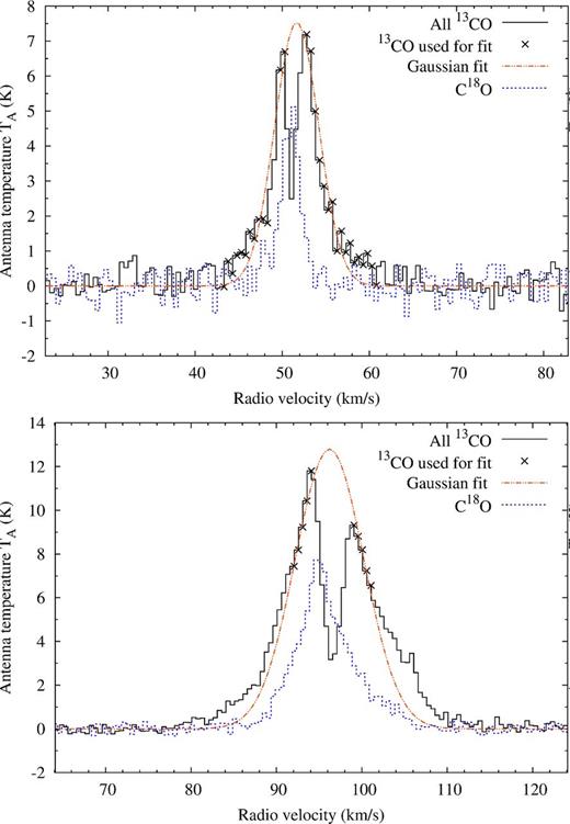
Gaussian fits (double dot–dashed lines) to the shoulders of 13CO spectra (crosses) towards G 22.038+0.222 (top) and G 28.201−0.049 (bottom), whose profiles show clear evidence of self-absorption. The Gaussian's peak is used as the estimated peak temperature. The C18O spectra (short dashed lines) give an indication where the actual peak is expected.
Following Codella et al. (2004), the optically thin C18O profiles were used as tracers for the line cores of targets. The C18O spectra were scaled to the 13CO peak temperature. To avoid subtracting any emission from higher velocity features that may be present in the C18O if densities were sufficiently high, a Gaussian was fitted to the C18O peak to approximate the line core-only emission. This was done by gradually removing points from the outer (higher velocity) edges of the C18O spectrum until the peak could be fitted, following the same approach as van der Walt, Sobolev & Butner (2007); see Fig. 3(a). The scaled Gaussian fit was then subtracted from the 13CO spectra to show the velocity ranges in the line wings where there is excess emission in 13CO.
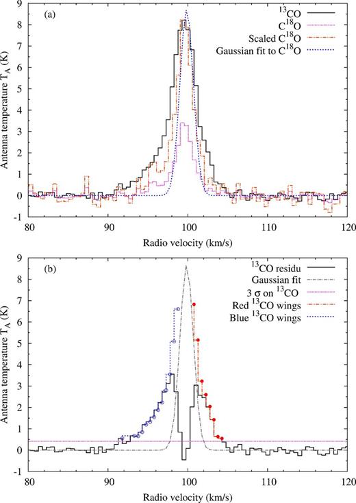
(a) Example of the 13CO spectrum (solid line) for the clump associated with maser G 28.321-0.011. Its C18O spectrum (dot–dashed line) is scaled to the 13CO peak (double dot–dashed line) and a Gaussian is fitted to the scaled spectrum (short dashed line). (b) The 13CO residuals following Gaussian subtraction is shown (solid line), along with the 3σ noise level (dotted line) and wing residuals satisfying the selection criteria. Blue wings are indicated by a short dashed line and empty circles, and red wings by a double dot–dashed line and solid circles.
G 23.010−0.411 is a special case with a double-peaked profile. Assuming that this is caused by two separate but closely associated clumps, we used two Gaussians, each fitted just to the highest velocity shoulder of each C18O line peak. Whenever absorption dips occur in the 13CO profiles, no natural profile peak existed. Instead, the C18O spectra were scaled to the peak of the previous Gaussian fitted to the 13CO.
This Gaussian was then subtracted from the 13CO profile. The line wings are defined by the sections where the 13CO profile is broader than the scaled Gaussian representing the C18O line core emission, provided the 13CO corrected antenna temperature is higher than 3σ (σ is the noise per 0.5 km s−1 channel, averaged over a 30 km s−1 section of the emission-free spectrum). An example of this wing selection process is shown in Fig. 3(b), which shows the 13CO residual spectrum and discrete spectral points that satisfy the wing criteria (empty circles are blue, and solid circles are red).
There is a risk that some blue and red emission might be missed by analysing a single spectrum at the location of the clump peak. Therefore, when the position of peak intensity in both the blue and red integrated images was found (mapping of blue and red images is explained in Section 3.3), another two additional spectra, called the ‘red-wing spectrum’ and ‘blue-wing spectrum’, were extracted. Once again blue and red residual spectra were calculated. If broader wing emission was found, the initial wing ranges were expanded to incorporate the ranges covered by the red-wing and blue-wing spectra. The final velocity ranges for blue and red wings are listed in Table 2.
Mapping the outflows
The final blue- and redshifted velocity ranges are used to produce two-dimensional 13CO intensity integrated images corresponding to each wing. These are overlaid as solid blue- and dotted red contours on to the 13CO-integrated intensity image, representing the outflow lobes. Two examples are shown in Fig. 4, showing target G 24.493−0.039 with the maser and clump coordinates overlapping, and target G 29.956−0.016A with an offset between the maser and clump coordinates. The remainder of the maps are shown online in Appendix B as Supporting Information. Contours are plotted in 10 per cent intervals up to 90 per cent of the maximum intensity, Intb or Intr, for each integrated image (values listed in columns 10 and 12 in Table 2). The lowest contour is never lower than 30 per cent, but values differ for each image depending on the individual background brightness levels. The lowest contour is selected by eye as the level which encompassed the outflow lobe clearly.
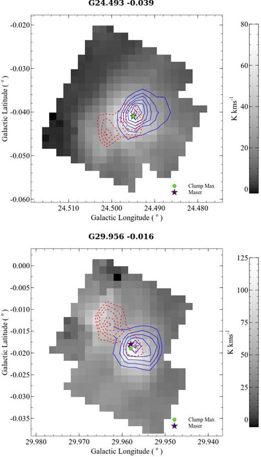
Two examples of intensity integrated images of the blue and red wing, from top to bottom: G 24.493−0.039 and G 29.956−0.016 (clump 1). Grey-scale image shows 13CO, integrated over the peak emission (velocity ranges listed in Table 1), with blue and red contours representing blue and red wing integrated intensities respectively. Contour intervals are 10 per cent of the maximum intensity for each image, increasing up to 90 per cent of the maximum intensity. Lower contours are, respectively, at 60 and 50 per cent for the two targets.
As massive stars form in clusters, the observed targets often have contamination from similarly HV components as the outflow, but from different spatial structures in the field of view (Shepherd & Churchwell 1996a). This makes it difficult to isolate the outflow. Therefore, if identified as belonging to such structures, these pixels were flagged to be bad in any further analysis. Sometimes one or both of the outflows are partially cut off where they are situated close to the edge of the field of view or to a dead receptor. These sources are flagged as such in the second to last column in Table 5 and their calculated properties only serve as a lower limit because a fraction of the emission is not included in the analysis.
Three of the 58 analysed clumps have been too close to the edge of the field of view for any significant information to be derived and are excluded from further analysis. Out of the remaining 55 maps, 47 outflows are clearly bipolar (85), with the eight exceptions marked with a superscript in Table 2. For a sample of high-mass protostellar objects, Beuther et al. (2002b) had a bipolar outflow detection frequency of 81 in 12CO, comparable with what we find.
RESULTS
Detection frequency
All of the 58 spectra available for analysis (see Section 3.1) were found to have HV outflow signatures, either in the spectra or in the contour maps, resulting in a 100 per cent detection rate. Such a high detection rate of outflows towards massive YSOs is not uncommon. Shepherd & Churchwell (1996b) searched for 12CO(J = 1-0) HV line wings towards 122 high-mass star-forming regions and detected low-intensity line wings in 94 of them. Of these 94, 90 per cent were associated with HV gas in the beam. The argument has already been made at that stage, that if the HV gas is due to bipolar outflows, molecular outflows are a common property of newly formed massive stars. Sridharan et al. (2002) detected 84 per cent of sources with HV gas from a 12CO |${\rm (J = 2{\rm -}1)}$| survey of 69 protostellar candidates.
Zhang et al. (2001, 2005) observed a sample of 69 luminous IRAS point sources in CO (J = 2-1) and detected 39 molecular outflows towards them (57 per cent). They found the search for outflows hampered for Galactic longitudes <50° (due to confusion my multiple cloud components when observing in this transition). A total of 39 objects were outside of this region, towards which 35 outflows were detected, resulting in a 90 per cent outflow detection rate.
Kim & Kurtz (2006) observed 12 sources from the same Molinari et al. (1996) catalogue that Zhang et al. (2001) selected their sources from. They detected outflows in 10 sources and adding these sources to the detections from Zhang, results in a detection rate of 88 per cent ([35 + 10 − 3 = 42] out of [39 + 12 − 3 = 48]), taking into account that there are three sources in common between the two samples. More recently, López-Sepulcre et al. (2009) searched for molecular outflows towards a sample of eleven very luminous massive YSOs. They found HV wings, indicative of outflow motions, in 100 per cent of the sample.
Three further studies have dealt specifically with class II methanol masers. Codella et al. (2004) surveyed for molecular outflows towards 136 UCHii regions, out of which 56 positions showed either 6.7 GHz methanol or 22.2 GHz water maser emission. Their overall outflow detection rate from 13CO(J = 1-0) and (J = 2-1) transition lines was ∼39 per cent, but they found that in cases where observations were made towards 6.7 GHz methanol or 22.2 GHz water maser emission lines, the outflow detection rate increased to 50 per cent. As their observations were single pointings, they may have missed some outflows that were offset from the masers. Xu et al. (2006) studied molecular outflows using high-resolution CO (J = 1-0) mapping towards eight 6.7 GHz methanol masers closer than 1.5 kpc. They found outflows in seven of them, an 88 per cent detection rate. Wu et al. (2010) investigated the distinctions between low- and high-luminosity 6.7 GHz methanol masers via multiline mapping observations of various molecular lines, including 12CO(J = 1-0), towards a sample of these masers. They found outflows to be common among both sets of masers: of the low-luminosity masers, they found six outflows out of nine, and from the high-luminosity masers they found four outflows out of eight, an overall detection rate of 59 per cent. Note that the detection frequencies from both Xu et al. (2006) and Wu et al. (2010) are obtained from small number samples.
All these results suggest that the majority of massive YSOs have molecular outflows, and should 6.7 GHz methanol masers be present, they are closely associated with the outflow phase.
Maser distances
Green & McClure-Griffiths (2011) published the kinematic distances for about 50 per cent of the targets in this study, using the 6.7 GHz maser mid-velocity as an estimate for the systemic velocity. They used respectively the presence/absence of self-absorption in H i spectra in the proximity of the systemic velocity, to determine whether the source is at the near/far kinematic distance. However, methanol maser emission often consists of a number of strong peaks spread over several km s−1. As differences of only a few km s−1 in the velocity of the local standard of rest vlsr can be enough to change the kinematic distance solution from near to far and vice versa in the H i absorption feature method of resolving the former, using estimated vlsr values form the maser emission could lead to an incorrect distance solution. Therefore, molecular line observations provide more reliable measurements of the clump systemic velocity (Urquhart et al. 2014).
For this reason, and to prevent the additional uncertainties introduced by adopting distances calculated using different techniques by different authors, we decided to recalculate all distances of the methanol masers using their associated C18O peak velocities. This was done using the Galactic Rotation Curve (GRC) as fitted by Brand & Blitz (1993), with the Sun's Galactocentric distance, R0, assumed as 8.5 kpc and its circular rotation Θ0 as 220 km s−1. Calculated values are listed in Table 3. The average difference between distances calculated using the GRC, versus the maser distances listed by Green & McClure-Griffiths (2011) for our targets, is 0.8 ± 0.6 kpc.
Target C18O velocities used to calculate their kinematic distances from the GRC (Brand & Blitz 1993). Literature references used to resolve the far/near distance ambiguities are listed in the fourth column, being an assembly from published 6.7 GHz masers, OH-masers, EGOs, IRCD's and molecular clouds. Sources with velocities within 10 km s−1 of the tangent velocity are placed at the tangent distance, indicated by TAN. Columns five to eight show information used in Section 4.4: the surface areas A for blue and red lobes as mapped in 13CO and lobe lengths l as measured from the clump coordinate to each outflow's radial extreme.
| Target | C18O v | D | Literature Reference | Ab | Ar | lb | lr |
|---|---|---|---|---|---|---|---|
| (km s−1) | (kpc) | (pc2) | (pc2) | (pc) | (pc) | ||
| G 20.081-0.135 | 41.602 | 12.6 | Fish et al. (2003) | 1.48 | 1.75 | 1.28 | 0.92 |
| G 21.882+0.013 | 20.158 | 1.8 | Purcell et al. (2006) | 0.06 | 0.05 | 0.29 | 0.23 |
| G 22.038+0.222 | 51.533 | 3.8 | Cyganowski et al. (2009) | 0.29 | 0.29 | 0.60 | 0.44 |
| G 22.356+0.066 | 84.189 | 5.2 | Green & McClure-Griffiths (2011) | 0.41 | 0.62 | 0.53 | 1.59 |
| G 22.435-0.169 | 27.895 | 13.4 | Roman-Duval et al. (2009) | 2.27 | 1.06 | 1.56 | 0.78 |
| G 23.003+0.124r | 107.445 | 6.2 | Roman-Duval et al. (2009) | – | 0.26 | – | 0.54 |
| G 23.010-0.411 | 76.380 | 4.8 | Green & McClure-Griffiths (2011) | 1.03 | 0.68 | 1.48 | 0.99 |
| G 23.206-0.378 | 77.829 | 10.7 | Green & McClure-Griffiths (2011) | 0.97 | 1.17 | 1.40 | 1.40 |
| G 23.365-0.291 | 78.292 | 4.9 | Roman-Duval et al. (2009) | 0.35 | 0.53 | 1.14 | 1.07 |
| G 23.437-0.184 | 100.630 | 5.9 | Green & McClure-Griffiths (2011) | 0.52 | 0.90 | 0.77 | 0.85 |
| G 23.484+0.097 | 84.181 | 5.2 | Simon et al. (2006) | 0.50 | 0.25 | 0.68 | 0.53 |
| G 23.706-0.198 | 69.090 | 11.1 | Green & McClure-Griffiths (2011) | 5.07 | 4.35 | 2.25 | 3.06 |
| G 24.329+0.144 | 112.743 | 7.7 | TAN | 0.86 | 0.81 | 1.01 | 0.68 |
| G 24.493-0.039 | 111.752 | 6.4 | Caswell & Green (2011) | 1.19 | 0.91 | 1.03 | 0.94 |
| G 24.790+0.083A | 110.548 | 9.1 | Green & McClure-Griffiths (2011) | 0.49 | 0.56 | 0.92 | 0.79 |
| G 24.850+0.087 | 108.941 | 6.3 | Roman-Duval et al. (2009) | 0.40 | 1.48 | 0.82 | 1.19 |
| G 25.650+1.050 | 42.315 | 12.3 | Green & McClure-Griffiths (2011) | 4.83 | 4.58 | 2.32 | 1.61 |
| G 25.710+0.044 | 101.214 | 9.4 | Green & McClure-Griffiths (2011) | 1.86 | 2.83 | 2.46 | 1.77 |
| G 25.826-0.178 | 93.206 | 5.5 | Green & McClure-Griffiths (2011) | 0.60 | 0.26 | 0.81 | 0.65 |
| G 28.148-0.004 | 98.665 | 5.9 | Green & McClure-Griffiths (2011) | 0.68 | 0.59 | 0.86 | 0.95 |
| G 28.201-0.049 | 94.860 | 9.3 | Green & McClure-Griffiths (2011) | 1.10 | 1.75 | 0.81 | 1.35 |
| G 28.282-0.359 | 47.354 | 3.2 | Green & McClure-Griffiths (2011) | 0.24 | 0.44 | 0.61 | 0.76 |
| G 28.305-0.387 | 85.627 | 9.8 | Green & McClure-Griffiths (2011) | 2.02 | 4.44 | 1.42 | 1.56 |
| G 28.321-0.011 | 99.570 | 6.0 | Roman-Duval et al. (2009) | 0.94 | 1.33 | 0.70 | 1.04 |
| G 28.608+0.018 | 103.075 | 7.5 | TAN | 0.80 | 1.23 | 1.09 | 1.09 |
| G 28.832-0.253 | 87.189 | 5.3 | Green & McClure-Griffiths (2011) | 1.31 | 0.48 | 0.93 | 0.69 |
| G 29.603-0.625r | 77.185 | 4.8 | Roman-Duval et al. (2009) | – | 0.54 | – | 0.84 |
| G 29.865-0.043 | 101.849 | 7.4 | TAN | 1.79 | 1.98 | 2.36 | 1.61 |
| G 29.956-0.016A | 97.838 | 7.4 | TAN | 1.51 | 1.19 | 1.18 | 1.61 |
| G 29.956-0.016B | 97.838 | 7.4 | TAN | 0.55 | 0.92 | 0.64 | 1.18 |
| G 29.979-0.047 | 101.843 | 7.4 | TAN | 0.96 | 0.87 | 1.29 | 0.64 |
| G 30.317+0.070 | 44.645 | 11.6 | Green & McClure-Griffiths (2011) | 1.83 | 1.49 | 1.52 | 1.52 |
| G 30.370+0.482A | 17.414 | 13.4 | Roman-Duval et al. (2009) | 3.03 | 1.36 | 1.95 | 1.36 |
| G 30.370+0.482B | 17.914 | 13.4 | Roman-Duval et al. (2009) | 2.58 | 1.67 | 2.92 | 1.17 |
| G 30.400-0.296 | 102.959 | 7.3 | TAN | 1.23 | 0.77 | 1.39 | 0.96 |
| G 30.419-0.232 | 104.549 | 7.3 | TAN | 0.73 | 1.59 | 2.00 | 2.03 |
| G 30.424+0.466 | 15.493 | 13.5 | Roman-Duval et al. (2009) | 4.64 | 4.95 | 3.74 | 2.36 |
| G 30.704-0.068b | 90.123 | 5.5 | Green & McClure-Griffiths (2011) | 0.49 | – | 0.40 | – |
| G 30.781+0.231 | 41.851 | 2.9 | Green & McClure-Griffiths (2011) | 0.13 | 0.09 | 0.29 | 0.25 |
| G 30.788+0.204 | 81.615 | 9.5 | Green & McClure-Griffiths (2011) | 2.55 | 1.16 | 1.39 | 0.83 |
| G 30.819+0.273r | 98.128 | 6.1 | Green & McClure-Griffiths (2011) | – | 0.58 | – | 0.80 |
| G 30.898+0.162r | 105.328 | 7.3 | TAN | – | 0.86 | – | 1.49 |
| G 30.973+0.562 | 23.396 | 12.89, 1.7 | – | 4.64, 0.08 | 2.25, 0.04 | 1.69, 0.22 | 1.12, 0.15 |
| G 30.980+0.216r | 107.365 | 7.3 | Roman-Duval et al. (2009) | – | 1.12 | – | 1.06 |
| G 31.061+0.094 | 19.227 | 13.2, 1.4 | – | 2.05, 0.02 | 0.29, 0.003 | 1.53, 0.16 | 0.96, 0.10 |
| G 31.076+0.457b | 28.310 | 12.5, 2.0 | – | 4.26, 0.11 | 3.59, 0.09 | 3.10, 0.50 | |
| G 31.122+0.063 | 41.528 | 11.7 | Roman-Duval et al. (2009) | 5.11 | 3.25 | 3.58 | 3.58 |
| G 31.182-0.148A | 42.648 | 11.6 | Roman-Duval et al. (2009) | 2.30 | 1.26 | 1.02 | 0.85 |
| G 31.282+0.062 | 109.028 | 7.3 | TAN | 1.61 | 1.16 | 1.58 | 1.27 |
| G 31.412+0.307 | 96.428 | 7.3 | TAN | 0.58 | 1.42 | 0.63 | 0.84 |
| G 31.594-0.192 | 43.149 | 11.6 | Roman-Duval et al. (2009) | 3.17 | 5.09 | 1.18 | 3.70 |
| G 32.744-0.075 | 37.528 | 11.7 | Green & McClure-Griffiths (2011) | 2.10 | 2.21 | 1.54 | 1.19 |
| G 33.317-0.360r | 34.814 | 11.8, 2.4 | – | – | 2.13, 0.09 | – | 1.38, 0.28 |
| G 33.486+0.040 | 111.986 | 7.1 | TAN | 0.17 | 0.64 | 0.52 | 1.13 |
| G 33.634-0.021 | 103.750 | 7.1 | TAN | 0.93 | 0.42 | 0.72 | 0.62 |
Alternative solutions to Brand & Blitz (1993) for calculating the kinematic distances are Reid et al. (e.g. 2009) and Clemens (1985). Urquhart et al. (2014) found that for sources in the inner Galaxy, the distances given, respectively, by these rotation curves, all agree within a few tenths of a kpc, which are smaller than their associated uncertainty of the order ±1 kpc due to streaming motions (Urquhart et al. 2011, 2012). Consequently, the statistical results are robust against the choice of model.
The galactocentric distances obtained using the GRC from Brand & Blitz (1993) were geometrically converted to heliocentric distances, of which two solutions exist within the solar circle, called the kinematic distance ambiguity (KDA). These distances are equally spaced on either side of the tangent position, and are generally referred to as the near and far distances. Sources with velocities within 10 km s−1 of the tangent velocity are placed at the tangent distance (indicated by TAN in the reference column), since the error in the distance is comparable to the difference between the near/far distance and the tangent distance.
As Green & McClure-Griffiths (2011) could resolve the KDA for many masers using corresponding H i self-absorption profiles, when available, we used their values to resolve the KDAs for our targets. Where maser distances were not published in Green & McClure-Griffiths (2011), alternative sources were used where available, being other publications of 6.7 GHz masers (Purcell et al. 2006; Caswell & Green 2011), EGOs (Cyganowski et al. 2009), OH-masers (Fish et al. 2003), associated IRDCs (Simon et al. 2006), or molecular clouds (Roman-Duval et al. 2009) – if the maser position fell within the cloud as well as within ∼ 5 km s− 1 of the cloud's vlsr – were used to resolve our KDAs. The literature reference used to resolve the distance for each source, should it exist, is also listed in Table 3.
For four out of the 58 targets, no published distance could be found to resolve the KDA. In these cases, both the near and far values are listed. Three targets are rejected from this list in Table 3: G 24.790+0.083B, because of too high noise, and G 30.851+0.123 and G 31.182−0.148B, because the clumps are mostly cut off by the edge of the field of view. The columns after the distance columns, list outflow lobe surface areas and lengths, values used for calculations discussed in Section 4.4.
Dealing with uncertainties
Calculation of the physical properties of molecular outflows can provide useful information on the obscured driving source. These calculations are subject to a number of uncertainties, most prominent of which is the outflow orientation. However, this is not easily determined (e.g. Shepherd & Churchwell 1996b; Curtis et al. 2010) and, as such, no correction is applied in this study. Although we will not apply any corrections, we discuss in the following paragraphs the corrections usually applied in the literature for outflow orientation. We also report the effects of such corrections on the calculated outflow properties, as well as additional contributors to uncertainties.
Our observations were some of the first to be carried out with the HARP instrument and some of the receptors exhibited poor performance and did not yield useful data. Often more than two receptors had to be switched off. At times this resulted in some of the clump/outflow emission being missed. Potentially, this could also result in outflow lobes not being detected at all. Blue and red contour levels were determined by eye, since each image is uniquely characterized by the background noise, emission brightness and available receptors. The 14 arcsec beam of the telescope places a limit on the size of outflows that can be resolved, especially for the more distant targets.
The most significant of the above uncertainties, is θ, the angle of the outflow axis with respect to the line of sight. As only a projection of the outflow is observed, any inclination with respect to the plane of sky will reduce the length of the outflow (not the width) by sin(θ), and increase the observed Doppler broadening by cos(θ). Cabrit & Bertout (1990) give a detailed discussion of the effect of inclination angle. Due to the lack of a specific orientation for each outflow, many authors assume a mean inclination angle for their sample to correct the calculated outflow parameters. The most commonly used angle is 57| $_{.}^{\circ}$|3, determined using the assumption that outflows are distributed uniformly and with random inclinations to the line of sight (Bontemps et al. 1996; Beuther et al. 2002b; Hatchell, Fuller & Richer 2007; Curtis, Richer & Buckle 2010). Table 4 summarizes the corrections due to inclination for the outflow parameters calculated (see Section 4.4). Unknown inclinations mostly cause the outflow parameters to be underestimated. Time-scales td are thus likely to represent a lower limit to the true age of the outflows (Parker, Padman & Scott 1991) and hence also to the time over which the embedded protostars responsible for the outflows have been accreting from their surroundings (Beuther et al. 2002b).
Inclination angle corrections on outflow parameters. All values in column 3 calculated for θ = 57| $_{.}^{\circ}$|3.
| Flow parameters | Correction | Corr. val. | Lit. val. |
|---|---|---|---|
| p | 1/cos(θ) | 1.9 | 2a, b, c |
| Em | 1/cos2(θ) | 3.4 | 3a, b, c |
| td | cot(θ) | 0.6 | ★d |
| |$\dot{M}_{{\rm out}}$| | tan (θ) | 1.6 | |
| Fm | sin(θ)/cos2(θ) | 2.9 | 3e, f |
| Lm | sin(θ)/cos3(θ) | 5.3 |
| Flow parameters | Correction | Corr. val. | Lit. val. |
|---|---|---|---|
| p | 1/cos(θ) | 1.9 | 2a, b, c |
| Em | 1/cos2(θ) | 3.4 | 3a, b, c |
| td | cot(θ) | 0.6 | ★d |
| |$\dot{M}_{{\rm out}}$| | tan (θ) | 1.6 | |
| Fm | sin(θ)/cos2(θ) | 2.9 | 3e, f |
| Lm | sin(θ)/cos3(θ) | 5.3 |
Note: *for 20° < θ < 70°, 0.4–2.7
Other contributors to uncertainties are possible difficulty separating the outflowing gas from the ambient gas; higher interstellar extinction towards the molecular ring in the inner Galaxy (0° < l < 50°) in addition to their internal extinction (Zhang et al. 2005); different CO/H2 abundance ratios used by different authors (e.g. Rodriguez et al. 1982; Cabrit & Bertout 1992; Herbst & van Dishoeck 2009).
Some authors use the mean atomic weight of the mixture of hydrogen and helium gas (Garden et al. 1991), while others only consider pure hydrogen molecular gas (Snell et al. 1984), resulting in a difference of 0.36 amu in the mean atomic weight (Wu et al. 2004). The excitation temperature, Tex, is assumed to range from 30 to 50 K for high-mass sources (Shepherd & Churchwell 1996b; Beuther et al. 2002b; Wu et al. 2004). However, a constant temperature assumption will underestimate the kinetic energy for an outflow with high jet/ambient density contrast (Downes & Cabrit 2007). Contamination from additional unrelated velocity components within the telescope beam could make it difficult to isolate the outflow, unless the components have a different spatial distribution from the outflow gas (Shepherd & Churchwell 1996a). Finally, even though we used 13CO as a tracer, we note that for their 12CO observations, Cabrit & Bertout (1990) estimated typical errors in the outflow parameters that reflect uncertainties in 12CO/H2, distance determinations, Tex, inclination angles, optical depth effects and possible low-level contamination of 12CO emission in the reference position. These error values are a factor ∼3 on outflow mass Mout, a factor ∼10 on mechanical force Fm, and a factor ∼30 on mechanical luminosity Lm.
Calculation of outflow physical properties
Physical properties of all blue and red outflow lobes as detected in 13CO. Where multiple clumps exist, their target labels are distinguished by ‘A’ and ‘B’. Both values are listed for sources with distance ambiguities, with (1) next to the target name indicating values for far distances, and (2) mark the values for near distances. Application of the 12CO/13CO scaling factor to wing velocity ranges will lead to a factor 2 increase in p and Fm and factor 4 increase in E and Lm. Column 11 lists any additional notes about the mapped lobes and column 12 indicates whether a target belongs to the MMAOs subset (as defined in Section 4.4) or not.
| Target | Mb | Mr | Mout | p | E | t | |$\dot{M}_{{\rm out}}$| | Fm | Lm | Notes | MMAO? |
|---|---|---|---|---|---|---|---|---|---|---|---|
| ( M⊙) | (M⊙) | (M⊙) | (M⊙ km s− 1) | (J) | (yr) | (|${\rm 10^{-4}\,\mathrm{M}_{{\odot }} \,\mathrm{yr}^{-1}}$|) | (M⊙ km s−1 yr) | (L⊙) | |||
| G 20.081−0.135 | 110 | 180 | 280 | 2700 | 1.5E+41 | 5.7E+04 | 50 | 4.6E−02 | 210 | B/R partly c.o. | Y |
| G 21.882+0.013 | 3 | 1 | 4 | 23 | 8.4E+38 | 2.6E+04 | 2 | 8.9E−04 | 3 | Big offset-X | N |
| G 22.038+0.222 | 12 | 18 | 30 | 170 | 7.3E+39 | 3.3E+04 | 9 | 5.3E−03 | 18 | Y | |
| G 22.356+0.066 | 10 | 4 | 14 | 70 | 2.0E+39 | 1.8E+05 | 1 | 3.8E−04 | 1 | Y | |
| G 22.435−0.169 | 55 | 16 | 71 | 240 | 5.8E+39 | 2.3E+05 | 3 | 1.0E−03 | 2 | Y | |
| G 23.003+0.124r | – | 3 | 3 | 13 | 3.6E+38 | 6.6E+04 | 1 | 1.9E−04 | 0 | No B | Y |
| G 23.010−0.411 | 74 | 31 | 100 | 1200 | 8.1E+40 | 6.4E+04 | 16 | 1.8E−02 | 100 | 2 peaks,1clump | Y |
| G 23.206−0.378 | 38 | 38 | 76 | 670 | 4.0E+40 | 5.8E+04 | 13 | 1.2E−02 | 57 | Y | |
| G 23.365−0.291 | 7 | 12 | 20 | 83 | 2.1E+39 | 1.3E+05 | 2 | 6.3E−04 | 1 | Y | |
| G 23.437−0.184 | 30 | 81 | 110 | 1100 | 6.6E+40 | 3.6E+04 | 31 | 3.1E−02 | 150 | Y | |
| G 23.484+0.097 | 10 | 6 | 16 | 82 | 2.7E+39 | 5.8E+04 | 3 | 1.4E−03 | 4 | B/R partly c.o. | Y |
| G 23.706−0.198 | 160 | 110 | 270 | 1100 | 2.8E+40 | 3.3E+05 | 8 | 3.4E−03 | 7 | R partly c.o. | Y |
| G 24.329+0.144 | 24 | 11 | 35 | 230 | 1.0E+40 | 6.0E+04 | 6 | 3.8E−03 | 14 | Y | |
| G 24.493−0.039 | 50 | 31 | 81 | 700 | 3.4E+40 | 7.2E+04 | 11 | 9.8E−03 | 39 | Y | |
| G 24.790+0.083A | 17 | 31 | 48 | 400 | 1.8E+40 | 6.7E+04 | 7 | 6.0E−03 | 23 | Y | |
| G 24.790+0.083B | – | – | – | – | – | – | – | – | – | Clump c.o.-X | N |
| G 24.850+0.087 | 12 | 30 | 42 | 170 | 3.6E+39 | 1.5E+05 | 3 | 1.1E−03 | 2 | R partly c.o. | Y |
| G 25.650+1.050 | 400 | 350 | 750 | 7600 | 4.6E+41 | 9.9E+04 | 76 | 7.8E−02 | 380 | Y | |
| G 25.710+0.044 | 110 | 110 | 220 | 880 | 2.9E+40 | 2.1E+05 | 10 | 4.2E−03 | 12 | Big offset-X | N |
| G 25.826−0.178 | 18 | 7 | 25 | 190 | 9.2E+39 | 4.4E+04 | 6 | 4.3E−03 | 17 | Y | |
| G 28.148−0.004 | 14 | 12 | 26 | 140 | 4.4E+39 | 6.9E+04 | 4 | 2.0E−03 | 5 | Y | |
| G 28.201−0.049 | 120 | 250 | 370 | 4400 | 3.4E+41 | 4.3E+04 | 86 | 1.0E−01 | 660 | Y | |
| G 28.282−0.359 | 16 | 37 | 53 | 340 | 1.3E+40 | 5.3E+04 | 10 | 6.5E−03 | 21 | Big offset-X, B/R partly c.o. | N |
| G 28.305−0.387 | 160 | 410 | 570 | 1700 | 3.5E+40 | 1.8E+05 | 32 | 9.3E−03 | 16 | R partly c.o. | Y |
| G 28.321−0.011 | 34 | 36 | 70 | 280 | 7.6E+39 | 8.2E+04 | 9 | 3.4E−03 | 8 | R partly c.o. | Y |
| G 28.608+0.018 | 63 | 51 | 110 | 920 | 4.7E+40 | 5.7E+04 | 20 | 1.6E−02 | 67 | B/R partly c.o. | Y |
| G 28.832−0.253 | 43 | 38 | 81 | 660 | 3.8E+40 | 4.8E+04 | 17 | 1.4E−02 | 66 | Y | |
| G 29.603−0.625r | – | 13 | 13 | 41 | 8.1E+38 | 1.0E+05 | 3 | 4.0E−04 | 1 | Big offset-X, no B | N |
| G 29.865−0.043 | 240 | 61 | 300 | 1900 | 6.5E+40 | 1.8E+05 | 16 | 1.0E−02 | 29 | B partly c.o. | Y |
| G 29.956−0.016A | 160 | 90 | 250 | 1800 | 7.6E+40 | 8.1E+04 | 31 | 2.2E−02 | 78 | Y | |
| G 29.956−0.016B | 8 | 13 | 21 | 180 | 8.4E+39 | 7.9E+04 | 3 | 2.3E−03 | 9 | Big offset-X | N |
| G 29.979−0.047 | 93 | 26 | 120 | 1100 | 6.6E+40 | 7.6E+04 | 16 | 1.4E−02 | 72 | Y | |
| G 30.317+0.070 | 42 | 25 | 67 | 320 | 9.1E+39 | 1.5E+05 | 5 | 2.1E−03 | 5 | R partly c.o. | Y |
| G 30.370+0.482A | 43 | 29 | 73 | 310 | 8.2E+39 | 2.4E+05 | 3 | 1.3E−03 | 3 | Y | |
| G 30.370+0.482B | 3 | 2 | 5 | 15 | 2.5E+38 | 7.1E+05 | 0 | 2.1E−05 | 0 | Big offset-X, B mostly c.o. | N |
| G 30.400−0.296 | 65 | 20 | 84 | 500 | 2.1E+40 | 9.0E+04 | 9 | 5.5E−03 | 20 | Y | |
| G 30.419−0.232 | 53 | 140 | 190 | 810 | 2.4E+40 | 1.3E+05 | 15 | 6.1E−03 | 15 | B mostly c.o. | Y |
| G 30.424+0.466 | 100 | 130 | 230 | 990 | 2.4E+40 | 3.8E+05 | 6 | 2.6E−03 | 5 | B/R partly c.o. | Y |
| G 30.704−0.068b | 67 | – | 67 | 200 | 9.1E+39 | 2.2E+04 | 61 | 9.1E−03 | 34 | RR-X red lobe | Y |
| G 30.781+0.231 | 4 | 4 | 8 | 24 | 4.6E+38 | 4.4E+04 | 2 | 5.5E−04 | 1 | Y | |
| G 30.788+0.204 | 76 | 48 | 120 | 830 | 3.3E+40 | 1.0E+05 | 12 | 8.2E−03 | 27 | Y | |
| G 30.819+0.273r | – | 11 | 11 | 59 | 1.9E+39 | 7.2E+04 | 3 | 8.2E−04 | 2 | No B | Y |
| G 30.851+0.123 | – | – | – | – | – | – | – | – | – | Clump c.o., Big offset-X | N |
| G 30.898+0.162r | – | 26 | 26 | 170 | 3.8E+39 | 2.9E+05 | 2 | 5.7E−04 | 1 | No B, RR-adapted shape | Y |
| G 30.973+0.562(1) | 250 | 58 | 310 | 590 | 9.0E+39 | 2.7E+05 | 11 | 2.1E−03 | 3 | N | |
| G 30.973+0.562(2) | 4 | 1 | 5 | 10 | 1.5E+38 | 3.6E+04 | 2 | 2.8E−04 | 0 | N | |
| G 30.980+0.216r | – | 19 | 19 | 850 | 4.7E+41 | 1.2E+05 | 3 | 7.3E−03 | 330 | B separated-X, partly c.o. | Y |
| G 31.061+0.094(1) | 110 | 1 | 110 | 780 | 2.9E+40 | 1.7E+05 | 7 | 4.7E−03 | 15 | Subresolution R | N |
| G 31.061+0.094(2) | 1 | 0 | 1 | 9 | 3.3E+38 | 1.8E+04 | 1 | 5.0E−04 | 2 | Sub-resolution R | N |
| G 31.076+0.457b(1) | 110 | – | 110 | 1500 | 1.1E+41 | 3.0E+05 | 7 | 5.1E−03 | 30 | Big offset-X, RR-X red lobe | N |
| G 31.076+0.457b(2) | 3 | – | 12 | 40 | 2.8E+39 | 3.8E+04 | 6 | 1.1E−03 | 6 | Big offset-X, RR-X red lobe | N |
| G 31.122+0.063 | 170 | 130 | 300 | 2000 | 7.8E+40 | 2.9E+05 | 10 | 6.9E−03 | 22 | B/R partly c.o. | Y |
| G 31.182−0.148A | 43 | 7 | 50 | 190 | 4.1E+39 | 1.7E+05 | 3 | 1.2E−03 | 2 | Y | |
| G 31.182−0.148B | – | – | – | – | – | – | – | – | – | Clump c.o.-X | N |
| G 31.282+0.062 | 73 | 42 | 110 | 810 | 3.1E+40 | 1.3E+05 | 9 | 6.2E−03 | 20 | Y | |
| G 31.412+0.307 | 15 | 58 | 73 | 680 | 3.3E+40 | 7.9E+04 | 9 | 8.6E−03 | 35 | Y | |
| G 31.594−0.192 | 47 | 120 | 160 | 600 | 1.2E+40 | 6.0E+05 | 3 | 9.9E−04 | 2 | R partly c.o. | Y |
| G 32.744−0.075 | 110 | 110 | 220 | 1700 | 7.6E+40 | 9.4E+04 | 24 | 1.8E−02 | 67 | Y | |
| G 33.317−0.360r(1) | – | 46 | 46 | 240 | 6.7E+39 | 1.7E+05 | 6 | 1.4E−03 | 3 | No B | N |
| G 33.317−0.360r(2) | – | 2 | 2 | 10 | 2.7E+38 | 6.8E+04 | 1 | 1.4E−04 | 0 | No B | N |
| G 33.486+0.040 | 1 | 7 | 8 | 19 | 3.1E+38 | 2.0E+05 | 0 | 9.6E−05 | 0 | Sub-resolution B | Y |
| G 33.634−0.021 | 37 | 9 | 46 | 110 | 2.2E+39 | 7.4E+04 | 6 | 1.5E−03 | 3 | Big offset-X, B partly c.o. | N |
Notes: key: R = red lobe, B = blue lobe; RR = red ridge; Offset = clump-maser coordinate offset; X = reject.
13CO is a less abundant molecule than 12CO, thus exhibiting a narrower spectral profile. A sample of 56 sources for which both 12CO and 13CO spectra were published has been investigated and the average 12CO/13CO full width zero intensity ratio is found to be ∼2 with a standard deviation of 1.3 (Cabrit, Goldsmith & Snell 1988; Shepherd & Churchwell 1996a; Su, Zhang & Lim 2004; Bronfman et al. 2008; Narayanan, Snell & Bemis 2012; Ortega et al. 2012; Xu & Wang 2013). All calculations containing wing velocities relative to the systemic velocity are scaled by this factor, implying a factor 2 increase in p and factor 4 increase in E.
For sources with unresolved distances, both values are shown and distinguished by the numbers next to the target names (1 = far and 2 = near). Exclusions are then made in further analyses for targets which have (i) kinematic distance ambiguities, hence uncertainties in calculated physical parameters, or, (ii) offsets of more than 3 pixels (18 arcsec, of the order of a beam size) between the maser coordinate and peak CO emission. These targets are marked as such in the notes of Table 5. Following the exclusions, we are left with 44 outflows in our sample that are positionally associated with methanol masers and for which we can calculate physical properties that are unaffected by distance ambiguities. We refer to this sample as MMAOs, indicated as such in Table 5, and base all further discussion on these outflows.
Clump masses
The evolutionary sequence of massive stars begins with prestellar clumps and cores, which are gravitationally bound overdensities inside a molecular cloud that show signs of inward motion before a protostar starts forming (Zinnecker & Yorke 2007; Dunham et al. 2011). Most massive stars form in star clusters (e.g. Clarke, Bonnell & Hillenbrand 2000; Lada & Lada 2003), which are part of a hierarchical structure, defined by Williams, Blitz & McKee (2000) and summarized by Bergin & Tafalla (2007). In this approach, the largest structure is a molecular cloud, with masses of the order 103–104 M⊙ and diameters ranging from 2 to 15 pc. Clouds contain subunits of enhanced density gas and dust, called clumps, wherein the earliest stages of massive star formation take place. Clumps will typically form stellar clusters (Williams et al. 2000).
Studies of massive star formation regions showed that clumps generally have sizes of the order of ∼1 pc, and masses ranging from order 10 M⊙ to ∼103–104 M⊙ (Kurtz et al. 2000; Smith, Longmore & Bonnell 2009). They are defined to be coherent in position–velocity space. Smith et al. showed that the gravitational potential of these clumps causes global collapse, which channels mass from large radii towards the centre of the cluster, where protostars with the greatest gravitational radius accrete it, causing them to become massive. Stars (or multiple systems such as binaries) eventually form from gravitationally bound subunits in the clumps, called cores (Williams et al. 2000). Cores have sizes typically ≤0.1 pc and masses ranging from 0.5 M⊙ up to ∼102–103 M⊙ (Kurtz et al. 2000; Smith et al. 2009).
We have corresponding C18O maps for 51 out of the 55 13CO maps. The optically thin C18O serves as a useful tracer of the central clump (e.g. López-Sepulcre et al. 2009). With a median source distance of 7.2 kpc and telescope beam of 14 arcsec, our resolving power is of the order of 0.5 pc, which, given the above definitions, implies the traced structures are more likely clumps than cores.
Coordinates and masses of the central clumps associated with the methanol masers, as derived from the 870 μm dust flux measurements from ATLASGAL (Csengeri et al. 2014). The last column lists the clump masses as calculated using C18O maps. (Suffixes ‘A’ and ‘B’ and numbers (1) and (2) next to some entries in column 1 have the same meaning as in Table 5).
| Target | Clump coord. | Dust flux | M870μm | |$M{_{\rm C^{18}O}}$| | |
|---|---|---|---|---|---|
| l(°) | b(°) | Sν (Jy) | (M⊙) | (M⊙) | |
| G 20.081−0.135 | 20.081 | −0.135 | 10.5 | 9200 | 1800 |
| G 21.882+0.013 | 21.875 | 0.008 | 3.7 | 65 | 20 |
| G 22.038+0.222 | 22.040 | 0.223 | 5.5 | 430 | 41 |
| G 22.356+0.066 | 22.356 | 0.068 | 5.4 | 810 | 64 |
| G 22.435−0.169 | 22.435 | −0.169 | 2.3 | 2300 | 200 |
| G 23.003+0.124 | 23.002 | 0.126 | 0.9 | 200 | 18 |
| G 23.010−0.411 | 23.008 | −0.410 | 12.8 | 1700 | 110 |
| G 23.206−0.378 | 23.209 | −0.378 | 11.1 | 7100 | 370 |
| G 23.365−0.291 | 23.364 | −0.291 | 5.0 | 660 | 47 |
| G 23.437−0.184 | 23.436 | −0.183 | 11.9 | 2300 | 490 |
| G 23.484+0.097 | 23.483 | 0.098 | 4.2 | 620 | 120 |
| G 23.706−0.198 | 23.706 | −0.197 | 3.9 | 2600 | 340 |
| G 24.329+0.144 | 24.330 | 0.145 | 9.0 | 3000 | 91 |
| G 24.493−0.039 | 24.493 | −0.039 | 12.0 | 2700 | 300 |
| G 24.790+0.083A | 24.790 | 0.083 | 26.6 | 12 000 | 670 |
| G 24.850+0.087 | 24.853 | 0.085 | 2.4 | 530 | 240 |
| G 25.650+1.050 | 25.649 | 1.051 | 16.6 | 14 000 | 2200 |
| G 25.710+0.044 | 25.719 | 0.051 | 0.6 | 300 | 250 |
| G 25.826−0.178 | 25.824 | −0.179 | 12.1 | 2100 | 120 |
| G 28.148−0.004 | 28.148 | −0.004 | 3.6 | 700 | 170 |
| G 28.201−0.049 | 28.201 | −0.049 | 15.7 | 7500 | 1800 |
| G 28.282−0.359 | 28.289 | −0.365 | 8.8 | 510 | 250 |
| G 28.305−0.387 | 28.307 | −0.387 | 4.3 | 2300 | 1200 |
| G 28.321−0.011 | 28.321 | −0.011 | 3.4 | 670 | 150 |
| G 28.608+0.018 | 28.608 | 0.018 | 5.2 | 1600 | 680 |
| G 28.832−0.253 | 28.832 | −0.253 | 9.5 | 1500 | 130 |
| G 29.603−0.625 | 29.600 | −0.618 | 2.5 | 310 | 53 |
| G 29.865−0.043 | 29.863 | −0.045 | 4.2 | 1300 | 630 |
| G 29.956−0.016A | 29.956 | −0.017 | 17.5 | 5200 | 900 |
| G 29.956−0.016B | 29.962 | −0.008 | 3.5 | 1000 | 27 |
| G 29.979−0.047 | 29.979 | −0.048 | 6.5 | 1900 | 170 |
| G 30.317+0.070 | 30.317 | 0.070 | 1.2 | 930 | 160 |
| G 30.370+0.482A | 30.370 | 0.484 | 1.2 | 1200 | 140 |
| G 30.400−0.296 | 30.403 | −0.296 | 1.9 | 570 | 120 |
| G 30.419−0.232 | 30.420 | −0.233 | 7.2 | 2100 | 290 |
| G 30.424+0.466 | 30.424 | 0.464 | 1.9 | 1900 | 950 |
| G 30.704−0.068 | 30.701 | −0.067 | 22.0 | 3700 | 790 |
| G 30.781+0.231 | 30.780 | 0.231 | 0.7 | 30 | 10 |
| G 30.788+0.204 | 30.789 | 0.205 | 5.9 | 3000 | 320 |
| G 30.819+0.273 | 30.818 | 0.273 | 1.8 | 380 | 53 |
| G 30.898+0.162 | 30.899 | 0.163 | 3.7 | 1100 | 140 |
| G 30.973+0.562(1) | 30.972 | 0.561 | 0.7 | 660 | 150 |
| G 30.973+0.562(2) | – | – | – | 11 | 3 |
| G 30.980+0.216 | 30.979 | 0.216 | 2.7 | 780 | 150 |
| G 31.061+0.094(1) | 31.060 | 0.092 | 1.0 | 930 | 130 |
| G 31.061+0.094(2) | – | – | – | 10 | 1 |
| G 31.076+0.457(1) | 31.085 | 0.468 | 1.5 | 1300 | 230 |
| G 31.076+0.457(2) | – | – | – | 34 | 6 |
| G 31.122+0.063 | 31.124 | 0.063 | 0.9 | 700 | 290 |
| G 31.182−0.148A | 31.182 | −0.148 | 1.1 | 830 | Too low S/N |
| G 31.282+0.062 | 31.281 | 0.063 | 13.1 | 3800 | 520 |
| G 31.412+0.307 | 31.412 | 0.306 | 29.8 | 8700 | 1000 |
| G 31.594−0.192(1) | 31.593 | −0.193 | 1.0 | 720 | 180 |
| G 32.744−0.075 | 32.746 | −0.076 | 7.8 | 6000 | 1100 |
| G 33.317−0.360(1) | 33.317 | −0.360 | 0.6 | 500 | Too low S/N |
| G 33.317−0.360(2) | – | – | – | 20 | Too low S/N |
| G 33.634−0.021 | 33.649 | −0.024 | 2.3 | 630 | 190 |
However, López-Sepulcre et al. (2009) noted that their dust clump masses are a factor ∼5 larger than the corresponding C18O masses, and stated that this difference might be explained by the fact that C18O and the submm continuum are tracing different parts of the clump. They found the angular full width at half-maximum (FWHM) measured in the submm continuum surveys to be a factor ∼2.5 larger than what is mapped by C18O (J = 2–1), and speculated that this played a main role in the difference between the two mass estimates. Hofner et al. (2000) also concluded from their survey that masses derived from submm dust emission, tend to be systematically higher than masses derived from C18O by a factor ∼2. They pointed out that contributing sources of uncertainty to this discrepancy could be C18O abundance, optical depth estimates, and the dust grain emissivity adopted.
Therefore, we also use continuum measurements to calculate the clump masses associated with MMAOs, and use the latter in all further discussions. The 870 μm flux measurements were obtained from the the APEX Telescope Large Area Survey of the Galaxy (ATLASGAL) survey (Schuller et al. 2009; Contreras et al. 2013), using offsets within a FWHM beam (beam size 19 arcsec) as matching criteria. Using the matching fluxes from Csengeri et al. (2014) for the targets in this study, clump masses were calculated following Urquhart et al. (2013a), with a gas-to-dust mass ratio assumed to be 100, dust absorption coefficient κν of 1.85 cm2 g−1 and dust temperature of 20 K. All values are listed in Table 6. Two clump masses are listed for sources with distance ambiguities, marked with (1) next to the name for the far distance, and (2) for the near distance. Excluding all targets with distance ambiguities, these clump masses range from ∼30 to 1.4 × 10⁴ M⊙, have a mean value of ∼(2.5 ± 0.5) × 103 M⊙ and median of ∼1.3 × 10³ M⊙. The clump masses associated with the MMAO subset have a mean of ∼2.8 × 10³ M⊙. For the targets with resolved distances, 96 per cent have masses >102 M⊙ and 49 per cent have masses of the order of 103–104 M⊙. This confirms that the majority of these targets are likely classified as clumps, as per definitions given above.
We find that the clump masses derived from dust measurements for our targets, are on average a factor 8 higher than masses derived using their C18O emission, in agreement with López-Sepulcre et al. (2009) and Hofner et al. (2000).
DISCUSSION
Clump and outflow mass relations
Here, we investigate the relationships between outflow properties and the mass of the clumps that they are associated with. While it is not possible to resolve the contribution from individual stars or protostellar cores in our data we can at least infer a relationship between clump mass and the most massive star present in the clump (e.g. Urquhart et al. 2013b).
McKee & Tan (2003) derived a relation for the accretion rate of a free-falling envelope as a function of time, wherein it is proportional to the clump surface density Σ0.75. This implies higher mass accretion in the most massive and dense clumps, compared to those forming in lower mass clumps. The former will arrive at the main-sequence sooner, and hence form an H ii region much more quickly than less massive stars forming in lower mass clumps. Urquhart et al. (2014) found their results to confirm this hypothesis, being consistent with the decreasing time-scale with increasing massive YSO luminosity found by Mottram et al. (2011).
In addition to this, Urquhart et al. also found that the most massive stars form predominantly towards the centres of their spherical, centrally condensed host clumps, where the highest densities exists and the gravitational potential is the deepest. These stars evolve much quicker than those outside the central region, and reach the main sequence in ∼105 yr, ahead of the lower mass stars which can take ∼10 times longer. Thus, while the most massive star, traced by the 6.7 GHz methanol maser in this study, is near to joining the main sequence, it is likely that the lower mass members of the protocluster still need to evolve to a stage where they make a significant contribution to the observed luminosity.
Urquhart et al. (2013b) found that for the H ii regions they investigated, the bolometric luminosities (which are effectively a measure of the whole protocluster luminosity), were very similar to values estimated from the radio continuum flux (which only trace the most massive stars). This suggests that it is likely that the bolometric luminosity is actually dominated by the most massive stars. Urquhart et al. (2014) also found that there is a strong correlation between the clump masses and the bolometric luminosities of the most massive stars, but that the total clump luminosities are much lower than would be expected from the fully formed cluster. These findings agree with the stated hypothesis, that the most massive stars have very rapid evolution times, and are consequently likely to dominate the observed clump properties. Thus, if the luminosity of a clump is dominated by the most massive stars, then it is reasonable to assume that so too, is the luminosity, and consequently the energetics, of the outflow.
In the following, we compensate for the loss of one lobe's mass in monopolar targets by doubling the values of the detected lobe for Mout, p, E, |$\dot{M}{_{\rm out}}$|, Fm and Lm, as they all depend on the outflow mass. Figs 5(a) and (b) shows the relation between, respectively, outflow masses and mass-loss rates, and clump masses for the MMAO sample (solid circles). In order to compare these relations with low-mass YSOs, we obtained associated outflow masses from Wu et al. (2004), Narayanan et al. (2012) and Davis et al. (2010) for 13 of the core envelope masses listed by Bontemps et al. (1996, empty circles). The pink squares represent the clump masses from Beuther et al. (2002a), derived from 1.2 mm dust continuum data, together with their associated outflow masses and mass-loss rates, as calculated in Beuther et al. (2002b). These values are corrected according to the erratum that was later published by Beuther et al. (2005), where the authors explain that their grain emissivity approximation should be a factor 2 higher than initially calculated, which would cause their derived clump masses to be a factor 2 lower than reported.
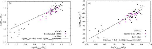
Relation between (a) outflow and clump masses and (b) outflow mass-loss rate and clump masses, for MMAOs (solid circles), with the best-fitting power laws shown. Empty circles indicate values for low-mass YSOs, with core envelope masses from Bontemps et al. (1996) and associated outflow mass and mass-loss rates from Wu et al. (2004), Narayanan et al. (2012) and Davis et al. (2010). Pink squares show the data from Beuther et al. (2002b).
In Fig. 5(a), a best-fitting power law to the MMAO sample (circles) is given by log(Mout/M⊙) = (−0.8 ± 0.3) + (0.8 ± 0.1)log(Mclump/M⊙), holding over three orders of magnitude for massive outflows, and extending towards the low-mass regime to cover six orders of magnitude in total.
López-Sepulcre et al. (2009) converted their clump masses derived from C18O to dust masses, and found a tight correlation between Mclump and Mout, described by Mout = 0.3M0.8clump. Sánchez-Monge et al. (2013) did a similar fit, but they calculated their outflow masses from SiO observations and clump masses from SED fits to the Hershel infrared Galactic Plane Survey (Hi-GAL) data. They found the same relation as López-Sepulcre et al. (2009). The power law found for MMAOs agrees with these authors within uncertainties. It is interesting to note that the outflow masses and mass-loss rates for MMAOs are generally higher than those estimated by Beuther et al. (2002b). We will discuss this property more detail in an upcoming second paper (de Villiers et al., in preparation).
Fig. 5(b) shows the best-fitting linear relation between the logarithmic values for the mass-loss rates and clump masses for MMAOs, given by |${\rm log}(\dot{M}_{{\rm out}}/{\mathrm{M}_{{\odot }} \,\mathrm{yr}^{-1}}) = (-5.0 \pm 0.4)+(0.6 \pm 0.1){\rm log}(M{_{\rm clump}}/{\mathrm{M}_{{\odot }}})$|. It again holds over three orders of magnitude for massive outflows, and extend to the low-mass regime to cover six orders of magnitude in total.
As both Mout and |$\dot{M}_{{\rm out}}$| depend on mass and distance, a nonparametric measure of the statistical dependence between these parameters and Mclump is needed. The Spearman-rank test is used, similarly to Ridge & Moore (2001), where a perfect positive or negative correlation exists between the ranks when rs is ±1. No correlation exists when rs = 0. The Spearman parameter rs is related to the two-tailed Student's t-test via, |$t_{\rm s} = r_{\rm s} \sqrt{(n-2)/(1-r^{2}_{\rm s})}$| for a sample size n. For no significant correlation, |$|t_{\rm s}| < |t_{s{_{\rm crit}}|}$|. For a sample size of 43 (MMAO sample of 44 had 43 matches from ATLAGAL for clump masses), |$t_{s{_{\rm crit}}}$| is ±2.02. The relation between Mout and Mclump for MMAOs is statistically significant with rs = 0.59 (ts = 4.66). The same is true for the relation between |$\dot{M}_{{\rm out}}$| and Mclump, where rs = 0.64 (ts = 5.28).
The result that both relations in Fig. 5 are found to hold over six orders of magnitude when extrapolated to the low-mass regime, suggests that a similar process causes outflows in both low- and high-mass star formation.
Fig. 6(a) shows the relation between the outflow mass and dynamical time-scales for MMAOs. A power law fitted to the data resulted in a poor correlation given by log(Mout/M⊙) = (0.3 ± 1.2) + (0.3 ± 0.3)log(t/ yr− 1), with rs = 0.18 (ts = 1.18, for a complete MMAO sample of 44) implying no significant correlation, as also found by Wu et al. (2004). Our range of dynamical times is possibly too small for any significant evolutionary trends, such as the increase in outflow mass, to be observed.
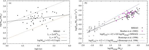
(a) Outflow masses versus dynamical time as derived from 13CO for MMAOs, with the best-fitting power law indicated by the solid line. Dot–dashed and dotted lines show, respectively, the lower and upper luminosity boundaries as defined by Shepherd & Churchwell (1996a). (b) Outflow mechanical force derived from 13CO versus associated clump masses for MMAOs (solid circles). The solid line is a power-law fit to MMAOs and the dotted line the fit from Bontemps et al. (1996). Empty circles represent this relation for low mass YSOs (Bontemps et al. 1996), and pink squares show the data from Beuther et al. (2002b).
Shepherd & Churchwell (1996a) plotted the same relation for their 10 massive star-forming regions. They divided their plot into three regions based on the bolometric luminosities of the outflow sources in Cabrit & Bertout (1992). We show the same luminosity boundaries in Fig. 6(a). Using data from Cabrit & Bertout (1992), Shepherd & Churchwell (1996a) found that sources with L* < 102 L⊙ were located below the bottom line and sources with L* > 2 × 10⁴ L⊙ above the top. This sectioning contributes a useful estimate of the expected bolometric luminosity of the YSO associated with each outflow studied – a property that could not be derived directly from the available data. Consistent with what is expected for massive YSO's, the majority (95 per cent) of the sources occur above the L* = 102 L⊙ boundary, with ∼79 per cent of them between L* = 102 L⊙ and L* = 2 × 10⁴ L⊙, and ∼16 per cent above L* = 2 × 10⁴ L⊙. Also, we find that higher luminosity (and hence more massive) YSOs will drive the higher mass outflows we study in this paper. A more massive accreting YSO is likely to have higher angular momentum, hence power larger outflows. In addition to this, star formation regions that form O and B stars tend to have larger reservoirs of material available to be entrained into a molecular outflow.
Fig. 6(b) shows the relation between the CO momentum flux/mechanical force FCO and the clump masses for MMAOs (circles), together with the values from Beuther et al. (2002b) (pink squares), as well as with 33 low-mass sources from Bontemps et al. (1996, triangles). FCO is the inclination corrected mechanical force, derived from Fm by applying a correction factor of 2.9, corresponding to a mean inclination angle of 57| $_{.}^{\circ}$|3 (i.e. assuming random outflow orientations, Beuther et al. 2002b and Table 4). Although we do not apply inclination corrections to the data in this study, in this specific case we correct Fm values in order to compare the CO momentum flux values from MMAOs with those from Beuther et al. (2002b) and Bontemps et al. (1996). Once again, as in Fig. 5, MMAOs’ momentum flux values are generally higher than those estimated by Beuther et al. (2002b, also to be discussed by de Villiers et al., in preparation).
The outflow's mechanical force is a very important parameter in studying the early phases of star formation. It is a measure of the rate at which momentum is injected from the underlying driving agent, via interactions with the molecular gas in the core, into the envelope. In other words, it is a measure of the outflow's strength and used to understand the driving mechanism of outflows (Bachiller & Tafalla 1999; Downes & Cabrit 2007). Hatchell et al. (2007) suggests that, although it is difficult to separate this effect from contamination due to the initial conditions, the correlation between FCO and Mclump suggests that the outflow activity declines during the later stages of the accretion phase (when the clump mass decreases).
Many authors have studied this relation before, both for low-mass outflows (e.g. Bontemps et al. 1996; Hatchell et al. 2007; Takahashi et al. 2008; Curtis et al. 2010; van der Marel et al. 2013) and high-mass outflows (e.g. Henning et al. 2000; Beuther et al. 2002b). For our massive MMAOs, we find the relation to be log(FCO/M⊙ km s−1 yr−1) = (−4.5 ± 0.4) + (0.8 ± 0.1)log(Mclump/M⊙) (black solid line) with a Spearman-rank coefficient of rs = 0.66(ts = 5.62). This relation found for MMAOs corresponds within uncertainties to what Bontemps et al. (1996) found for low-mass sources, log(FCO/M⊙ km s−1 yr−1) = −(4.2 ± 0.1) + (1.1 ± 0.2)log(Mclump/M⊙) (blue dotted line).
If, as stated in the beginning of this section, the outflow energetics are dominated by the most massive cores in a clump harbouring massive star formation, the presence of the same relationship between the outflow parameters and the clump masses for both high and low masses, is consistent with the theory that massive star formation is an scaled-up version of the low-mass scenario.
Mass-loss rate and accretion rates
If massive outflows are produced by the same mechanism as low-mass outflows, it implies that the outflows are momentum driven by the jet coming from the central YSO which entrains the surrounding molecular gas and forms the outflow. One of the proposed solutions, enabling disc accretion to be a possible formation process for massive stars, is when accretion proceeds through a disc with a high enough mass accretion rate to overcome the radiation pressure of the central massive star (Jijina & Adams 1996; Yorke & Sonnhalter 2002). Even more involved disc accretion models including asymmetric configurations and Rayleigh–Taylor instabilities (Krumholz, Klein & McKee 2007; Krumholz et al. 2009), assume accretion rates of the order of 10− 4 M⊙ yr− 1. High accretion rates (∼10−5–10−3 M⊙ yr−1) are also used in more recent disc accretion models that incorporate a dust sublimation front and consequently yielded the growth of the highest mass stars ever formed in multidimensional radiation hydrodynamic simulations (Kuiper et al. 2010).
The mean |$\dot{M}{_{\rm out}}$| for MMAOs is ∼1.7 × 10⁻³ M⊙ yr−1, which would lead to accretion rates of ∼3 × 10⁻⁴ M⊙ yr−1, being of the same order of magnitude as the ∼10−4 M⊙ yr−1 found by both Beuther et al. (2002b) and Kim & Kurtz (2006). Our approximate accretion rate for MMAOs is also much higher than typical accretion rates of |${\rm 10^{-7}\hbox{--}10^{-5} \,\mathrm{M}_{{\odot }}\,\mathrm{yr}^{-1}}$| expected for low-mass YSOs (Shu 1977), and agrees with the theoretical rates used in disc accretion models for massive stars (Krumholz et al. 2007; Kuiper et al. 2010).
Comparison with methanol masers
Integrated 6.7 GHz flux densities (Si) are obtained from the MMB catalogue (Breen et al., in preparation) for 38 of the MMAO masers. Using the distance of each target, Si is converted to an integrated spectral luminosity L6.7 GHz.
Fig. 7 shows the relation between the outflow mechanical luminosities (or energy supply rates) and maser luminosities for 38 masers from the MMAO subset, given as log(Lm/ L⊙) = (3.2 ± 1.3) + (0.2 ± 0.2)log(L6.7 GHz/ L⊙) and a Spearman-rank coefficient of rs = 0.28(ts = 1.78), which, although not quite, is at the margin of being statistically significant as the 5 per cent acceptance interval for t is ±2.02.
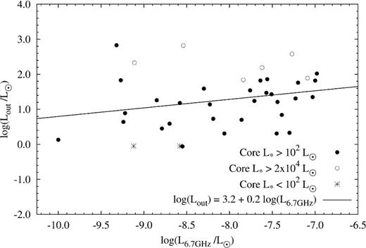
Outflow mechanical luminosities Lm derived from 13CO plotted versus 6.7 GHz maser luminosities. The solid line indicates the best-fitting power law to the data. Empty circles indicate sources located above the 2 × 10⁴ L⊙ bolometric luminosity boundary in Fig. 6(a), solid circles are sources located between the L* = 102 L⊙ and L* = 2 × 10⁴ L⊙ boundaries, and star symbols indicate sources located below L* = 102 L⊙.
Furthermore, following their positions in Fig. 6(a), we divide all the outflows plotted in Fig. 7 into three categories; outflows associated with clumps whose luminosities above 2 × 10⁴ L⊙, between the L* = 102 L⊙ and L* = 2 × 10⁴ L⊙, and below L* = 102 L⊙. The data points in Fig. 7 are marked accordingly. Although bright outflows are mostly associated with bright clumps, and low-luminosity outflows associated with lower luminosity clumps, there is no such preference for maser brightness.
Finally, we plot the relation between the 6.7 GHz maser luminosities against clump masses in Fig. 8 and found the best-fitting linear relation between the logarithmic values of these parameters to be log(L6.7 GHz/ L⊙) = ( − 10.6 ± 0.7) + (0.8 ± 0.2)log(Mclump/M⊙). The associated value for rs is 0.59 (ts = 4.36), which implies a statistically significant positive correlation.
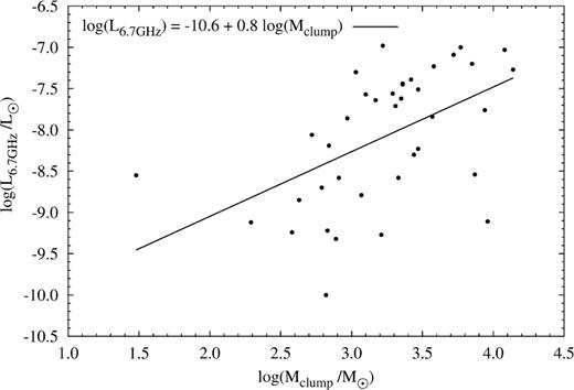
6.7 GHz maser luminosities versus clump masses derived from 870 μm continuum emission.
Breen et al. (2010) studied the relation between 101 1.2 mm dust clumps and their associated 6.7 GHz methanol masers. Their study showed that more luminous 6.7 GHz methanol masers are likely to be associated with dust clump sources that have bigger radii, higher mass and lower clump densities (the latter possibly due to the assumption of a constant dust temperature). These results are represented graphically in their fig. A2. Wu et al. (2010) also found molecular clumps (derived from NH3 lines) associated with high-luminosity 6.7 GHz masers to be larger and ∼10 times more massive than those associated with low-luminosity masers. They also found that outflows associated with high-luminosity masers have wider line wings and larger sizes than those associated with low-luminosity masers. This lead to their interpretation that masers with higher luminosities are associated with YSOs with larger masses.
Urquhart et al. (2013a) found a weak linear correlation between the maser luminosity and clump masses for 442 ATLASGAL–MMB associations. They speculated that this correlation may be related to the fact that the most massive clumps are likely to form more massive stars, and that a higher isotropic maser luminosity is somehow related to a higher stellar luminosity.
The results from Figs 8 and 7 agrees with above authors and suggest that there is some correlation between the mass (hence also brightness) of a massive YSO and both the luminosity of the outflow it generates as well as the total 6.7 GHz maser luminosity it pumps. Note that in this case, we know that a higher maser luminosity could not be due to a larger number of masers in more massive regions, as all our MMB-sample selected masers have supporting interferometric observations that reveal they are principally single-maser spots.
SUMMARY AND CONCLUSIONS
We analysed the 13CO and C18O spectra extracted at 58 13CO clump coordinates towards 6.7 GHz methanol maser coordinates between 20° < l < 34°. All spectra showed HV outflow signatures. Of these, the HV emission was mapped for 55 with 47 showing bipolar structures. A subset containing 44 targets is referred to as MMAOs, with the criteria that all members have to have resolved kinematic distances and be closely associated with a methanol maser. Only MMAOs were used for further analysis.
The wing spectra and spatial maps were used to calculate the physical properties of all 55 mapped outflows, generally following Beuther et al. (2002b), with a few adjustments in their approach for this study. The associated clump masses for MMAOs were calculated from the 870 μm flux measurements towards these targets, of the ATLASGAL survey (Csengeri et al. 2014).
The main results for this study can be summarized as follows. (i) A statistically significant relation over three orders of magnitude was found between the outflow and clump masses for the MMAOs, given by log(Mout/M⊙) = (−0.8 ± 0.3) + (0.8 ± 0.1)log(Mclump/M⊙). This relation agreed, within uncertainties, with Beuther et al. (2002b), López-Sepulcre et al. (2009) and Sánchez-Monge et al. (2013). Low-mass sources (Bontemps et al. 1996; Wu et al. 2004; Davis et al. 2010; Narayanan et al. 2012) were found to follow a similar trend as the massive sources, expanding the power-law relationship to over six orders of magnitude.
(ii) The relation between the outflow mass-loss rate and clump masses was described by |${\rm log}(\dot{M}_{{\rm out}}/{\mathrm{M}_{{\odot }} \,\mathrm{yr}^{-1}}) = (-5.0 \pm 0.4)+(0.6 \pm 0.1){\rm log}(M{_{\rm clump}}/{\mathrm{M}_{{\odot }}})$|, which held over six magnitudes down to the low-mass regime.
(iii) When plotting outflow masses against dynamical time-scales, 95 per cent of the MMAOs occurred above the L* = 102 L⊙ boundary for YSO luminosities, with ∼79 per cent of them between L* = 102 L⊙ and L* = 2 × 10⁴ L⊙, and ∼16 per cent above L* = 2 × 10⁴ L⊙. This suggests that higher luminosity (and hence more massive) YSOs will generate higher mass outflows.
(iv) The relationship between the mechanical force (CO momentum flux) FCO and the clump masses was described by log(FCO/M⊙ km s−1 yr−1) = (−4.5 ± 0.4) + (0.8 ± 0.1)log(Mclump/M⊙), a trend which held over six orders of magnitude if we included low-mass outflows.
(v) We derived an approximate accretion rate of ∼3 × 10⁻⁴ M⊙ yr−1 from our mean mass-loss rate. This is of the same order of magnitude than both the mean accretion rates found by Beuther et al. (2002b) and Kim & Kurtz (2006) and agrees with the theoretical rates used in disc accretion models for massive stars (Krumholz et al. 2007; Kuiper et al. 2010).
(vi) An investigation of the relation between the outflow mechanical luminosities and maser luminosities for 38 MMAO targets showed a weak positive correlation wherein bright outflows were associated with brighter masers and clumps. However, low-luminosity outflows and clumps showed no preference for maser brightness. The relation between the 6.7 GHz maser luminosities and clump masses was given by log(L6.7 GHz/ L⊙) = ( − 10.6 ± 0.7) + (0.8 ± 0.2)log(Mclump/M⊙). Although weakly correlated, these relations suggest that there is a correlation between the mass (hence also brightness) of a massive YSO and both the luminosity of the outflow it generates as well as the 6.7 GHz maser it pumps. It agrees with the speculation from Urquhart et al. (2013a) that such a correlation may be related to the fact that the most massive clumps are likely to form more massive stars, and that a higher isotropic maser luminosity is somehow related to a higher stellar luminosity.
Results (i), (ii) and (vi) indicate that both the outflow mass relations and energetics follow a common relation for low- and high-mass YSOs. This lends evidence to the hypothesis that a similar process is responsible for outflows in both mass regimes, i.e. high-mass star formation is a scaled-up version of the low-mass scenario. In addition to this, result (v) shows that the approximate mass accretion rate for MMAOs is sufficiently high to overcome the radiation pressure of a massive central star.
Although this evidence suggests that massive stars form in a similar fashion to low-mass stars, to determine whether each massive YSO indeed drives its own outflow, high-resolution imaging is required.
In a following paper (de Villiers et al., in preparation), the outflow property distributions are compared to those from other surveys, focusing on the evolutionary sequence of 6.7 GHz methanol masers and molecular outflows during the hot core phase.
We want to thank James Caswell for useful comments and contributions to the paper. Timea Csengeri acknowledges financial support for the ERC Advanced Grant GLOSTAR under contract no. 247078. The JCMT is operated by the Joint Astronomy Centre on behalf of the STFC of the United Kingdom, the National Research Council of Canada, and (until 2013 March 31) the Netherlands Organization for Scientific Research. The programme ID for the observations is M07AU20. We also thank the anonymous referee for constructive comments on the paper.
REFERENCES
SUPPORTING INFORMATION
Additional Supporting Information may be found in the online version of this article:
Appendix A
Appendix B (Supplementary Data).
Please note: Oxford University Press is not responsible for the content or functionality of any supporting materials supplied by the authors. Any queries (other than missing material) should be directed to the corresponding author for the paper.
