


Abstract
The static and transient deformations produced by earthquakes cause density perturbations which, in turn, generate immediate, long-range perturbations of the Earth's gravity field. Here, an analytical solution is derived for gravity perturbations produced by a point double-couple source in homogeneous, infinite, non-self-gravitating elastic media. The solution features transient gravity perturbations that occur at any distance from the source between the rupture onset time and the arrival time of seismic P waves, which are of potential interest for real-time earthquake source studies and early warning. An analytical solution for such prompt gravity perturbations is presented in compact form. We show that it approximates adequately the prompt gravity perturbations generated by strike-slip and dip-slip finite fault ruptures in a half-space obtained by numerical simulations based on the spectral element method. Based on the analytical solution, we estimate that the observability of prompt gravity perturbations within 10 s after rupture onset by current instruments is severely challenged by the background microseism noise but may be achieved by high-precision gravity strainmeters currently under development. Our analytical results facilitate parametric studies of the expected prompt gravity signals that could be recorded by gravity strainmeters.
1 INTRODUCTION
Earthquakes generate transient and static deformation, including volumetric deformation and displacement of material interfaces, which modify the spatial distribution of material density. This mass redistribution induces changes in the Earth's gravitational field. Permanent gravity changes generated by static deformation induced by the co-seismic and post-seismic slip of large earthquakes have been observed by superconducting gravimeters and gravity field satellite missions on multiple occasions (Imanishi et al.2004; Wang et al.2012a; Fuchs et al.2013; Cambiotti & Sabadini 2013). Theoretical models of these static gravity perturbations have been developed (Okubo 1992; Sun et al.2009) and compared to observations (Matsuo & Heki 2011; Wang et al.2012b). The transient effects of elasto-gravitational coupling on the Earth's gravest normal modes are well established and routinely included in normal mode computations for long-period seismology (Dahlen & Tromp 1998). Transient perturbations of the gravity field concurrent with the passage of seismic waves have been examined as a broad-band source of so-called Newtonian noise for gravitational-wave (GW) detectors (Beker et al.2011; Driggers et al.2012). Here we address, for the first time, the problem of modelling the gravity perturbations generated by earthquakes at short timescales, including those generated by transient deformation induced by seismic waves and those occurring during the fault rupture.
Our focus here is on a particular short-term elasto-gravitational effect that has received no attention in the literature. Owing to the long-range and virtually instantaneous (speed-of-light) effect of gravitational forces, density perturbations lead immediately to global perturbations of the Earth's gravity field. In particular, the volumetric deformation carried by P waves induces remote gravity perturbations even at distances beyond the P-wave front. Hence, at any distance from an earthquake source and its dynamically deforming region, gravity perturbations are expected to be induced even between the onset time of the rupture and the arrival time of seismic waves. We refer to these as prompt gravity perturbations. If practically measurable, these signals would add a new dimension to real-time seismology that may enhance rapid earthquake source detection and parameter estimation capabilities and may contribute to earthquake and tsunami early warning. Some analogies may be drawn to prompt electromagnetic perturbations caused, in principle, by earthquakes via the electrokinetic effect in saturated porous media (Gao et al.2013) or via the motional induction effect of the Earth's conductive crust and magnetic field (Gao et al.2014). Here we develop building blocks for the quantitative analysis of prompt gravity perturbations, as needed to assess their detectability and information content. An analysis of their potential contribution to earthquake early warning will be reported elsewhere, as well as results of a search for prompt gravity signals in superconducting gravimeter recordings of a recent mega-earthquake.
While normal mode theory in global seismology accounts for gravitational effects (Takeuchi & Saito 1972; Dahlen & Tromp 1998), the structure of the prompt gravity perturbation field is not immediately evident from it. To facilitate systematic, parametric studies of transient gravity signals, we develop in Section 2 an analytical model of transient Newtonian gravity perturbations from point shear dislocations in unbounded, uniform, non-self-gravitating elastic media. The model accounts for the effects of density perturbations induced by both static and transient deformations and provides a complete gravity time-series, before and after the passage of seismic waves. The key result is a compact expression for prompt gravity perturbations. Its relevance in more realistic settings is assessed in Section 3 by comparing the analytical results with results from numerical simulations that include finite fault and free surface effects. In Section 4, after realizing that prompt gravity perturbations are generally too weak to be detected by conventional gravimeters within 10 s after rupture onset, we derive expressions for transient gravity gradients and assess the theoretical potential of high-sensitivity gravity strainmeters to observe prompt gravity signals.
2 GRAVITY PERTURBATIONS FROM POINT-SHEAR DISLOCATIONS IN INFINITE, HOMOGENEOUS, NON-SELF-GRAVITATING ELASTIC MEDIA
2.1 Model assumptions and density perturbations
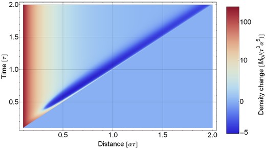
Density perturbation field as a function of distance and time, for ϕ = 0, θ = π/4 and seismic moment time function M0 tanh (t/τ)Θ(t), where Θ( · ) denotes the unit step function. Since the positive and negative values vary over many orders of magnitude, the colour scale is based on a log-modulus transformation (John & Draper 1980).
2.2 Prompt gravity perturbation
Prompt gravity perturbations are essentially the exterior gravitational field induced by the density perturbation outside its spatial support, that is, beyond the P-wave front. Their structure can be determined by exploiting classical results in potential theory (Jekeli 2007) as follows. The density perturbation field inherits the symmetries of a quadrupole from the P-wave radiation pattern, which features four lobes of alternating signs. A quadrupole density perturbation generates an exterior gravitational potential, which has also a quadrupole structure and decays as |$1/r_0^3$|, where r0 is the distance to the centroid of the quadrupole.
In this section, we use seismic potentials (of the seismic fields and alternatively of the seismic sources) to obtain an explicit expression of the gravity perturbation in homogeneous space valid for all times. In the Appendix, a second method is described, which uses the spherical multipole expansion. While the method based on potentials is not very intuitive and does not give a direct interpretation of the effective source of gravity perturbations, it is more elegant and should prove useful also to solving more complicated calculations in the future, for example concerning gravity perturbations in a half space.
The derivation, in particular eq. (9), has the unintuitive feature that the prompt gravity potential perturbation appears to emerge from the ‘acausal’ component of the P-wave potential. This component has actually no physical significance in the seismic wave equation, where its contribution to the near-field seismic wavefield is cancelled out by a similar contribution from the S-wave potential.
3 COMPARISON WITH SPECTRAL ELEMENT SIMULATIONS
The theory developed in Section 2 does not capture all effects that may be present in nature. Even if for some purposes the Earth can be sufficiently approximated by a homogenous medium, it remains to be determined under which conditions this theory adequately describes finite fault sources in a half space.
First, the theoretical results are derived for a point source. Additional finite-source effects are expected close to a finite-size rupture. We do not consider this a major drawback, since the problem is linear and finite-sized sources of arbitrary shape and with complicated rupture propagation can be represented by superposition of point sources. A suitable approximation to describe finite-size ruptures on a single planar fault is proposed here. The prompt gravity perturbation in that scenario is a superposition of quadrupole gravity fields, each of the form given by eq. (12). The leading term of the multipole expansion of a superposition of quadrupoles is also a quadrupole, whose quadrupole moment is simply the sum of the individual ones. The higher order multipole terms (octupole, etc.) are not necessarily zero but they decay faster with distance. Hence, at a distance from the P-wave front, the prompt gravity perturbation produced by a finite earthquake source is approximately given by eq. (12) if, as conventionally in seismology, M0(t) is understood as the seismic moment integrated over the whole finite rupture surface. To minimize the octupole contribution, r0 should be understood as the distance to the instantaneous earthquake centroid (or, more generally, to the instantaneous centroid of the density perturbation field). The quality of this approximation is expected to degrade as the P-wave front approaches.
Secondly, the analytical solution was derived for infinite media. If an event occurs at a depth h, then we can expect deviations from our results as soon as P waves reach the surface at time h/α, which is typically a few seconds only. Therefore, simulating many tens of seconds of gravity time-series using the analytical results of Section 2 would in general lead to inaccurate predictions. However, for early warning applications of prompt gravity signals the important question is if the influence of the surface is significant within a few seconds of the rupture onset.
The assumed kinematic source model is specified in Appendix B. It represents a circular pulse-like rupture of finite duration τ with cosine slip rate function, uniform final slip δ, rise time T and constant rupture speed vrup. From the rupture model, an explicit expression of the moment function M0(t) is obtained that is inserted into eq. (18) to calculate an analytical prediction of the gravity perturbation. We present results of three simulations, a very deep strike-slip event, a shallow one and a shallow dip-slip event, and compare them with the analytical predictions. The duration of the strike-slip events is τ = 2 s, while the duration of the dip-slip event is 4 s. The rise time in all cases is T = 1 s. We simulated about 5 s of time-series, a short timescale relevant to anticipated applications in early warning. It is computationally expensive to increase the simulation duration and at the same time increase the size of the simulation domain to encompass the complete P-wave front and preserve accuracy at high frequencies. Further parameter values of the simulations are listed in Table 1. For the strike-slip scenarios, the total ruptured area is A = π(vrupτ)2 and the seismic moment M0 = μδA. In the dip-slip scenario the rupture reaches the surface.
Parameter values used for the comparison between the numerical simulation and theory.
| Parameter | Symbol | Value |
|---|---|---|
| Rupture speed | vrup | 3 km s−1 |
| P-wave speed | α | 6.4 km s−1 |
| Mass density | ρ0 | 2670 kg m−3 |
| Shear modulus | μ | 27 GPa |
| Slip | δ | 0.5 m |
| Strike-slip events | ||
| Total ruptured area | A | 110 km2 |
| Total seismic moment | M0 | 1.5 × 10¹⁸ N m |
| Moment magnitude | Mw | 6.1 |
| Dip-slip event | ||
| Total ruptured area | A | 400 km2 |
| Total seismic moment | M0 | 5.4 × 10¹⁸ N m |
| Moment magnitude | Mw | 6.5 |
Fig. 2 shows the comparison between theory and simulation for the deep strike-slip event with hypocentre at 50 km depth. We compare the gravity acceleration in the horizontal direction normal to the fault evaluated at a horizontal distance of 1 km to the epicentre and to the fault (to avoid a null of gravity acceleration) and 2 km above ground (to avoid exponentially decaying artefacts of the gravity calculation related to the finite grid density). The relative deviation (shown as dashed line) grows with time but stays smaller than 7 per cent over the entire 5 s. This serves as verification of our SPECFEM3D implementation and to show that finite source effects are not significant at this distance.
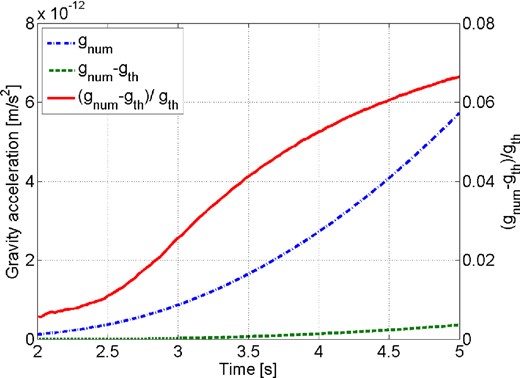
Comparison between analytical predictions gth and numerical simulation gnum of prompt gravity acceleration perturbations for a deep strike-slip earthquake. The solid curve is plotted against the right y-axis, while the dashed and dash-dotted curves are plotted against the left y-axis. The hypocentre is 50 km deep so that surface effects are non-existent during the first 5 s. The detector is located at a horizontal distance of 1 km from the epicentre to avoid a null of gravity acceleration. The result shows that approximating the fault rupture as a point source leads to relative deviations smaller than 0.07 within the first 5 s.
Fig. 3 (left) shows the comparison for the shallow strike-slip event with hypocentre depth 7.5 km. Gravity is evaluated at 50 km horizontal distance to the epicentre and 2 km above ground. The horizontal distance was chosen larger than the propagation distance of seismic waves during the first 5 s. The plot in the right of Fig. 3 shows the comparison for the 7.5 km deep dip-slip event with 45° dip angle, and 4 s duration. In these two examples, the relative deviation is smaller than 1.5 and 6 per cent, respectively. This is even smaller than in the previous example, which may seem surprising given that at t = 5 s seismic waves have already been reflected from the surface or have been converted into surface waves, which was not considered in the theoretical analysis. Especially concerning the dip-slip event, one might have expected more significant deviations since the surface experiences a differential lift across the fault trace when the rupture reaches the surface at about t = 3.5 s. The agreement between the theoretical and numerical results even in this case may be taken as a hint of a more fundamental principle that is to be discovered in the full half-space solution.
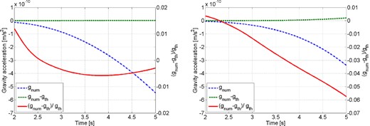
Comparison between analytical predictions gth and numerical simulation gnum of prompt gravity acceleration perturbations for a shallow strike-slip earthquake and a surface-breaking dip-slip earthquake. Same representation as in Fig. 2. Left: strike-slip event with 2 s duration. Right: dip-slip event with dip angle of 45° and duration of 4 s. In both cases, the event hypocentre is 7.5 km deep so that surface effects can be expected shortly after 1 s, and the detector is located at 50 km distance from the epicentre so that seismic waves do not reach it within the 5 s of simulation time. For the dip-slip scenario, the rupture reaches the surface at about 3.5 s. The impact of the surface onto gravity perturbations stays weak within the first 5 s, leading to relative deviations smaller than 0.015 for the strike-slip event, and 0.06 for the dip-slip event.
Strong deviations between theory and numerical simulations were only observed for shallow events in cases where gravity was evaluated close to the epicentre so that the contribution from passing Rayleigh waves was dominant. An open question that should be addressed in future studies is whether results still agree well even long after 5 s, at least as long as contributions from passing Rayleigh waves can be excluded. The effect of heterogeneity of the crust also deserves further scrutiny.
4 TRANSIENT GRAVITY GRADIENTS
4.1 Motivations
The past two decades have seen rapid progress in the development of ultra-sensitive gravity strainmeters, mainly driven by scientific communities working on GW detection from astrophysical sources. Gravity strain is the relative change in physical distance between two test masses in response to a changing gravitational field. This change can be produced by a GW of astrophysical origin as well as by gravity perturbations from terrestrial sources. Laser-interferometric GW detectors such as LIGO (LIGO Scientific Collaboration 2009), Virgo (Accadia et al.2011), GEO600 (Lück et al.2010), and KAGRA (Aso et al.2013) measure gravity strain as differential displacement between seismically isolated test masses using high-power, in-vacuum lasers. Strain sensitivities of better than 10− 22 Hz− 1/2 have been demonstrated in the frequency range between about 50 and 1000 Hz. The LIGO and Virgo detectors are currently being upgraded to advanced configurations with design strain sensitivity better than 10− 23 Hz− 1/2 between about 30 Hz and 2000 Hz. Furthermore, future ground-based detectors have been proposed, such as the Einstein Telescope (ET Science Team 2011) with even more enhanced strain sensitivity, and a detection band extending down to a few Hz. In parallel to these kilometre-scale detectors, groups are developing gravity strainmeters targeting signals below 1 Hz, which are better suited to detect gravity perturbations changing over timescales of a few seconds (Ando et al.2010; Hohensee et al.2011; Dickerson et al.2013; Shoda et al.2014).
In the next section, we derive expressions for gravity strain perturbations (expressed as gravity gradients, i.e. the second time derivative of gravity strain) useful to assess the capability of future sensors to observe prompt gravity signals. Current concepts and sensitivity goals of these ‘low-frequency’ instruments are briefly reviewed in Section 4.4.
4.2 Gravity-gradient tensor
4.3 Gravity-strain response
The instruments anticipated to observe weak gravity transients of the form given in eq. (28) measure changes in distance between test masses or relative rotations between suspended bars. These instruments measure the so-called gravity-strain tensor|${\mathsf {h}}\equiv I_2[{\mathsf {D}}](t)$|, rather than the gravity-gradient tensor |${\mathsf {D}}$|. The concept of gravity strain is similar to that of elastic strain. While elastic strain determines the relative change in distance between test masses bolted to an elastic medium, gravity strain causes a relative change in distance between freely falling test masses. The concept of gravity strain is predominantly used in the GW community, and since it emerged from studies of gravity in the framework of general relativity, it should also be emphasized that some of the predicted effects on instruments cannot be explained by Newtonian gravity theory. Nonetheless, in the context of this paper, it is sufficient to understand gravity strain as if produced by a tidal force and therefore it can be calculated from the gravity-gradient tensor by double integration as stated above.
4.4 Sensitivity of low-frequency gravity strainmeters
We conclude with a brief discussion about instruments and instrumental concepts potentially able to detect the gravity transients from earthquakes discussed in this work. Several concepts have been proposed for gravity strainmeters that target signals between 10 mHz and 10 Hz. These include atom-interferometric, laser-interferometric, torsion-bar, and superconducting gravity strainmeters (Moody et al.2002; Harms et al.2013). While none of the concepts has reached the sensitivity yet required for the detection of earthquake transients, sensitivities of 10−15 Hz−1/2 in the region 0.1–1 Hz seem within reach. Correspondingly and according to eq. (33), transient gravity signals from earthquakes at ∼10 s after rupture onset and at epicentral distances ∼50 km can be expected to have high signal-to-noise ratio. We point out that these low-frequency strainmeters are much smaller scale (of the order of 1 to 10 m) than the km-scale GW detectors LIGO and Virgo, which operate at higher frequencies. In fact, some of the modern concepts of low-frequency gravity strainmeters evolved from well-known gravity gradiometer technology. We also want to emphasize that the sensitivity of low-frequency gravity strainmeters required for the detection of earthquake transients lies well below the sensitivity required for GW detection at the same frequencies, which is about 10−19 Hz−1/2 at 0.1 Hz (Harms et al.2013). So it is conceivable that these instruments can be either early prototypes of future GW detectors, or instruments specifically built for geophysical observations.
Groups working on the realization of these new concepts rely on modern understanding of terrestrial gravity noise, seismic isolation, and thermal noise acquired over the past decade. For seismic-noise suppression, each concept follows a different strategy. Atom-interferometric detectors use freely falling ultracold atom clouds, and seismic noise couples strongly suppressed into the system through the laser interacting with the atoms (Baker & Thorpe 2012). Superconducting gravity strainmeters achieve seismic-noise reduction by common-mode suppression by differential readout of test-mass displacements versus a common rigid reference (Moody et al.2002). Laser-interferometric concepts rely on active and passive seismic isolation of suspended test masses (Harms et al.2013). Torsion-bar detectors profit from the mechanical filtering of seismic noise through a potentially very low frequency torsion resonance (Ando et al.2001). In reality, isolation performance is impeded by cross-coupling between degrees of freedom allowing seismic noise to couple into the strainmeter output through unwanted channels. The goal is to improve the mechanical designs to suppress these couplings.
As explained by Harms et al. (2013), terrestrial gravity noise is expected to pose sensitivity limitations at a level 10−15 Hz−1/2 at 0.1 Hz mainly due to atmospheric infrasound, and possibly also seismic fields (depending on the instrument site). It was proposed to use microphone or seismometer arrays to coherently cancel associated gravity fluctuations from the strainmeter data. However, this technique is mostly unexplored and therefore its performance is difficult to predict. Some experience has been gained with the cancellation of atmospheric gravity noise in gravimeter data (Neumeyer 2010), but gravity-noise cancellation in gravity gradiometers is not equivalent to cancellation in gravimeters.
The best strain sensitivity at 0.1 Hz so far has been demonstrated with superconducting gravity strainmeters reaching 10−10 Hz−1/2 (Moody et al.2002). Torsion-bar sensitivities have surpassed 10−7 Hz−1/2 at 0.1 Hz (Shoda et al.2014). Naturally, work on detector designs needs to be accompanied by careful selection of instrument sites, which can have a big impact on ambient seismic or infrasound fields (Berger et al.2004; Brown et al.2014), and also on the associated gravity noise.
5 CONCLUSION
In this paper we addressed for the first time the problem of modelling transient gravity perturbations produced by an earthquake during fault rupture. Since gravity changes propagate essentially instantaneously in comparison with seismic waves, gravity perturbations are generated at any distance as soon as the rupture starts. In particular, a prompt gravity perturbation is expected before the arrival of P waves, and has been computed here by an original analytical model, validated with numerical simulations. The model indicates that it would be challenging to observe prompt gravity signals within 10 s of the rupture onset with current instruments, but that they may be within the reach of high-precision gravity strainmeters currently under development.
This study sets building blocks to evaluate the detectability and information content of prompt gravity perturbations. The analysis of a potential application to earthquake early warning will be reported elsewhere, in which a few seconds of gravity signal would enable warning significantly faster than conventional systems based on seismic data. The detection of prompt gravity perturbations may also open new directions in earthquake seismology, since it consists in a direct measurement of the mass redistribution during fault rupture. How complementary is the information about the earthquake source contained in the transient gravity field and in seismic waves remains to be assessed.
Further analysis is needed to extend this study to cases where the Earth's surface affects more significantly the gravity perturbation field. Surface effects can be studied numerically, as was done here, but an analytical model of gravity perturbations in the presence of a surface would provide further insight.
We thank Eric Clévédé for discussions during the initial phase of this study and Mauricio Fuentes for assistance with verification and simplification of analytical derivations. This work was supported by NSF Grants PHY 0855313 and PHY 1205512 to UF. BFW acknowledges sabbatical support from the Université Paris Diderot and the CNRS through the APC, where part of this work was carried out. JPA acknowledges support by a grant from the Gordon and Betty Moore Foundation to Caltech. We acknowledge the financial support from the UnivEarthS Labex program at Sorbonne Paris Cité (ANR-10-LABX-0023 and ANR-11-IDEX-0005-02) and the financial support of the Agence Nationale de la Recherche through the grant ANR-14-CE03-0014-01.
SPECFEM3D is available at http://www.geodynamics.org/cig/software/specfem3d.
