


Abstract
The representation of viscoelastic media in the time domain becomes more challenging with greater bandwidth of the propagating waves and number of travelled wavelengths. With the continuously increasing computational power, more extreme parameter regimes become accessible, which requires the reassessment and improvement of the standard ‘memory variable’ methods to implement attenuation in time-domain seismic wave-propagation methods. In this paper, we propose a method to minimize the error in the wavefield for a fixed complexity of the anelastic medium. This method consists of defining an appropriate misfit criterion based on a first-order analysis of how errors in the discretized medium propagate into errors in the wavefield and a simulated annealing optimization scheme to find the globally optimal parametrization. Furthermore, we derive an analytical time-stepping scheme for the memory variables that encode the strain history of the medium. Then we develop the coarse grained memory variable approach for the spectral element method (SEM) and benchmark it using the 2.5-D code AxiSEM for global body waves up to 1 Hz. Showing very good agreement with a reference solution, it also leads to a speedup of a factor of 5 in the anelastic part of the code (factor 2 in total) in this 2.5-D approach. A factor of ≈15 (3 in total) can be expected for the 3-D case compared to conventional implementations.
1 INTRODUCTION
Ongoing advances in supercomputer architecture and numerical methods enable the solution of the wave equation in increasingly extreme parameter regimes, such as higher frequency waves in larger modelling domains, having longer propagation distances in terms of the number of travelled wavelengths. Numerical errors as well as errors in physical approximations accumulate over these larger distances and require more precision both in the numerical solution and in the physical medium representation. We address the question of how accurate attenuation and the corresponding physical dispersion needs to be represented to accurately model seismic waves including attenuation with a focus on global body waves, although the treatment is more general and scale invariant. Even though the quality factor Q is itself poorly constrained by existing seismic studies, especially its 3-D structure and frequency dependence (Romanowicz & Mitchell 2007, and references therein), we consider it an essential pre-requisite to carefully evaluate the accuracy of the numerous numerical and physical approximations, before upscaling conventional methods of implementing attenuation to the more extreme regimes that modern computational seismology approaches.
While moving from purely elastic to viscoelastic media is easy in the frequency domain via the correspondence principle and introduction of complex-valued media properties, it is more involved in the time domain since the multiplication in the constitutive relation of the elastic medium needs to be replaced by a convolution. A first method to transform the stress–strain relation into a differential form using Padé approximations is introduced by Day & Minster (1984). Later, Emmerich & Korn (1987) and Carcione et al. (1988) suggested to improve this by approximating the medium properties with a discrete relaxation spectrum (Liu et al.1976) and fitting the parameters used to describe this spectrum to the observed behaviour numerically. These methods are still common today (e.g. Komatitsch & Tromp 2002b; Graves & Day 2003; Kristek & Moczo 2003; Käser et al.2007; Fichtner et al.2009; Savage et al.2010), a more complete summary and historical overview is given by Carcione (2007) and Moczo et al. (2014). In this study, we suggest several improvements to this scheme leading to better accuracy in the medium representation at zero extra cost.
Even if Q is large [on the global scale the minimum observed value is about 50, Gung & Romanowicz (2004)] and the effect of attenuation on the seismograms small, accounting for it typically leads to an increase of the computational costs by a factor of two to four in both computation time and memory (e.g. Blanch et al.1995; Käser et al.2007). Day (1998) suggested a method called the coarse-grained memory variable approach to redistribute the medium properties on the subwavelength scale such that it behaves the same for the wavefield, but is computationally significantly less expensive. Day's method was originally developed for the acoustic wave equation and regular grid finite-difference schemes. It is generalized to the viscoelastic wave equation and improved by more appropriate averaging schemes by Day & Bradley (2001) and Graves & Day (2003). Kristek & Moczo (2003) further improved the scheme by introducing material-independent memory variables to avoid artificial averaging of material parameters at gridpoints where interpolation of the memory variables is necessary (e.g. in the context of heterogeneous finite-differences methods at material discontinuities or for thin layers). Ma & Liu (2006) apply the coarse-grained method to a low-order finite-element scheme on unstructured grids. However, their approach cannot directly be translated to higher-order methods such as the spectral element method (SEM), because in such schemes the elements are too large compared to the wavelength (less than four elements per wavelength). We propose to redistribute the medium properties within the elements on the high-order basis functions, which again is small scale compared to the wavelength.
On the global scale, high-frequency body waves are routinely observed at propagation distances of 1000–2000 wavelengths and more, a regime that is hardly accessible with current global 3-D solvers and computers (Carrington et al.2008). While the methods we propose for parameter optimization are completely general and the coarse-grained memory variable approach applicable to all high-order finite-element methods, we use the axisymmetric SEM AxiSEM introduced by Nissen-Meyer et al. (2007a,b, 2008), further developed to include anisotropy by van Driel & Nissen-Meyer (2014) and published open source by Nissen-Meyer et al. (2014) as an example implementation to test our theoretical arguments. The efficiency of this 2.5-D approach allows very high-frequency simulations (currently up to 2 Hz on the global scale) that are still impossible to reach using full 3-D methods, so it provides a good basis to test common physical and numerical approximations.
Other axisymmetric approaches to global and local wave propagation have been presented (Alterman & Karal 1968; Igel & Weber 1995, 1996; Chaljub & Tarantola 1997; Furumura et al.1998; Thomas et al.2000; Takenaka et al.2003; Toyokuni et al.2005; Jahnke et al.2008), but only recently Toyokuni & Takenaka (2006, 2012) generalized their method to include moment tensor sources, attenuation and the Earth's centre. These methods are all based on isotropic media and especially the finite-difference methods among them have to deal with large dispersion errors for interface-sensitive waves such as surface waves and diffracted waves (Igel & Weber 1995; Igel et al.1995). We generalize AxiSEM to viscoelastic anisotropic axisymmetric media to overcome these issues. This enables the simulation of high-frequency body waves with a particularly high sensitivity to attenuation, travelling distances over thousands of wavelengths such as transmitted, reflected and diffracted core phases.
2 THEORY
Here, we introduce the concepts and our notation for time-domain modelling of the memory variable approach to viscoelastic dissipation. We start with the simple 1-D case (scalar instead of tensorial quantities) and generalize to the full 3-D problem subsequently.
2.1 Preliminaries
Arbitrary frequency dependency of Q can hence be approximated by a sum of absorption bands (see Fig. 2), by tuning the 2N parameters of the discrete relaxation spectrum aj and ωj. This is one non-linear optimization problem for each set of Q and M in the model. It is important to note that this optimization is subject to the additional non-linear constraint aj > 0 [equivalent τϵ > τσ for the Zener model, compare Carcione (2007), eqs. 2.169 and 2.193].
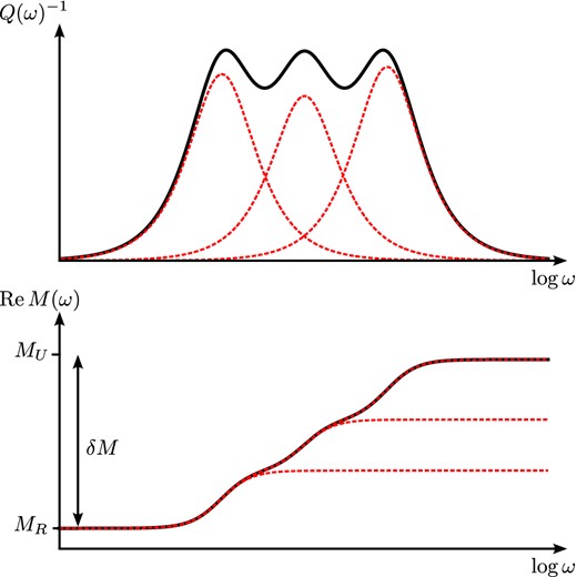
Inverse quality factor Q−1 and real part of the modulus M for a medium with three standard linear solids (see eqs 6 and 7). Dashed red lines indicate contributions from the individual linear solids, black solid lines the sum. Arbitrary frequency dependency (here: constant Q/logarithmic M in a limited frequency range) can be approximated by a sum of absorption bands. In the limit of large Q these take the form of Debye functions.
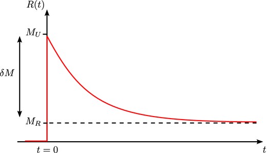
An important consequence of causality are the Kramers–Kronig relations stating that the real and imaginary part of M(ω) are related by Hilbert transforms. The medium is therefore fully described by either the modulus or the phase velocity at a reference frequency ωr, and the quality factor in the frequency range of interest Q(ω), which in practice is often assumed to be constant or obey a power law.
A basic question is then what criterion to use in order to find the parametrization of the medium for a numerical solution to the wave equation. We strive to optimize this procedure by means of the maximal error tolerance in the wavefield as defined by amplitude and phase error estimates in the next section.
2.2 Optimal Q parametrization
In this section, we analyse the influence of deviations in M(ω) and Q(ω) on the wavefield. As discussed, the optimization problem of finding the best set of 2N parameters is inherently non-linear (also for large Q due to the free choice of relaxation frequencies) and has a non-linear constraint. Taking this as given, choosing a non-linear optimization approach such as simulated annealing also enables the free choice of optimization criteria. The goal of this section is to define such a criterion for finding the material parametrization for the discrete relaxation spectrum that minimizes the error in the wavefield.
where nλ denotes number of propagated wavelengths and |$\frac{\Delta Q}{Q}$| and |$\frac{\Delta M_1}{M_1}$| are the relative errors in quality factor and real part of the modulus. As expected intuitively, the phase error is determined by the error in the real part of the modulus, which for large Q dominates the phase velocity, while the error in amplitude is determined by the error in Q.
Fig. 3 shows how the acceptable errors in the real part of the modulus and Q can be determined based on the phase and amplitude errors that are acceptable in a given application. For global high-frequency body waves (t* = Tr/Q = 4s, nλ = 1000) and an acceptable error of a few per cent in phase and amplitude, we conclude that Q should be approximated to well below 1 per cent and the modulus below 0.03 per cent. In contrast, the same seismic phase observed at lower frequencies, that is, smaller nλ = 100 as typically used in full 3-D global simulations, is well represented with errors in Q and modulus that are 10 times larger.
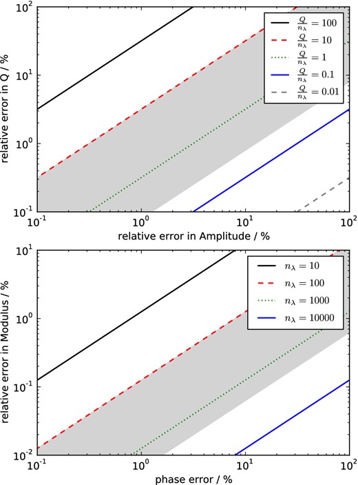
Given acceptable amplitude (top panel) or phase (bottom panel) error, what are the requirements for the parametrization of the anelastic medium in terms of acceptable error in quality factor Q and modulus M for a range of number of travelled wavelengths nλ. Shaded areas indicate typical global body waves, that is, t* = 1–4 s, period 1–10 s, traveltime 1000–2000 s. Note the different scales on the y-axis.
2.2.1 Optimization criteria and variables
It is common practice (Emmerich & Korn 1987; Blanch et al.1995; Komatitsch & Tromp 2002b; Graves & Day 2003; Kristek & Moczo 2003; Käser et al.2007; Savage et al.2010) to find the medium parametrization aj, ωj by choosing the relaxation frequencies ωja priori, mostly logarithmically spaced in the frequency range of interest. Then, the aj can be found by sampling Q(ω) at a finite number of frequencies ωk and solving an overdetermined inverse problem. We propose the following three-fold strategy to improve the parametrization: (1) a specific choice of the norm for the afore-mentioned inverse problem, (2) invert for ωj instead of setting them a priori and (3) fit the medium more accurately at the higher frequencies.
Fig. 4 visualizes the importance of including the relaxation frequencies in the optimization: for log-spaced fixed frequencies, the discretization of the medium does not converge towards the analytical behaviour, neither for increased N nor for smaller bandwidth for which the medium is optimized. This is in contrast to the finding by Savage et al. (2010), Fig. 2, whose results we are only able to reproduce when ignoring the constraint aj > 0. For applications where fitting of Q better than 1 per cent is needed (this is low Q or many wavelength propagation as for global high-frequency body waves, compare Fig. 3), inversion for the relaxation frequencies is inevitable. This non-linear optimization problem with 2N parameters can effectively be solved by a simulated annealing approach within seconds using 105–107 iterations for N ≤ 6, this was also suggested by Liu & Archuleta (2006).
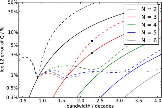
Importance of the choice of relaxation frequencies for a good approximation of constant Q for various numbers of absorption bands N as a function of bandwidth: frequencies fixed log-spaced (dashed lines) versus inversion using simulated annealing (solid line). Note that for fixed relaxation frequencies Q does not converge towards the optimal value, neither for larger N, nor for smaller bandwidth, and the minimal error is about 1 per cent. The dots correspond to the first two examples in Fig. 5.
Fig. 5 shows three examples of seismograms calculated with different medium representations that have the same numerical complexity in time-domain wave-propagation solvers due to the same number of memory variables. Both the reference solution and the approximations are calculated using the dissipation operator, the difference is only in M(ω). The first column represents the standard method of choosing the relaxation frequencies of the absorption bands log-spaced. Inverting for the frequencies can reduce both the misfit in Q and consequently phase and amplitude errors of the seismograms in all frequency bands by factors of 2–4 (second column). Additional frequency weighting reduces the phase and envelope misfit by another factor of 2 in the highest frequency band at the cost of worse fit in the lower frequency range (third column), resulting in same order of magnitude misfits in all frequency bands.
![Influence of the parametrization of the medium on the accuracy of the seismograms simulated with dissipation operators for t* = 4 s [typical for teleseismic S waves, see for example, Nolet (2008)] while keeping the complexity of the parametrization constant (three absorption bands). Left to right: relaxation frequencies fixed log-spaced in the frequency band of interest (2.3 decades), optimized frequencies using simulated annealing, additional linear weighting with the frequency. Top to bottom: seismograms filtered with Gabor-bandpass filters with centre period Tc, quality factor Q, modulus M and relative error of the modulus as approximated with standard linear solids. EM and PM denote the envelope and phase misfit (Kristekova et al.2009). Shaded region indicates the frequency range used in the parameter optimization, vertical dashed lines the relaxation frequencies ωj and solid black lines the reference medium. Optimization criterion was the log-l2 error of Q, see text for details. Note the large deviations of the optimal value in the modulus at the boundaries of the frequency range.](https://oup.silverchair-cdn.com/oup/backfile/Content_public/Journal/gji/199/2/10.1093/gji/ggu314/3/m_ggu314fig5.jpeg?Expires=1716451074&Signature=LKe~dnJbPC2K9YNRzFyAie8qs~KMBMzp1hPgThVK7sSNjhdyEHr4O5Fu8m1xX6di1~Ln9SjiJY3U2wC2dMYBri99--erQ~otIrcq0lx7jGcxQmiv4o5s~~4UW77cjGMRlffwuTTpazG3veEnlBdGhtf~O~L-Ds724J5iZJwmJhsR-apuZOebS3IfL47O3fTHTZP0n9ZWrk2QM9br5fbfb-J-0JfwmsfWiOYF1GzrjFsnHzDP~S9hVL1Hw0l7oj9isjPjZEme4QEVeN5t6lwuMPoMY3hD49zZP0VSWZBcbJVJTV7MmotrGq-aPpA5PKvgDBzvJQ9OU3T9nn7oSIi16g__&Key-Pair-Id=APKAIE5G5CRDK6RD3PGA)
Influence of the parametrization of the medium on the accuracy of the seismograms simulated with dissipation operators for t* = 4 s [typical for teleseismic S waves, see for example, Nolet (2008)] while keeping the complexity of the parametrization constant (three absorption bands). Left to right: relaxation frequencies fixed log-spaced in the frequency band of interest (2.3 decades), optimized frequencies using simulated annealing, additional linear weighting with the frequency. Top to bottom: seismograms filtered with Gabor-bandpass filters with centre period Tc, quality factor Q, modulus M and relative error of the modulus as approximated with standard linear solids. EM and PM denote the envelope and phase misfit (Kristekova et al.2009). Shaded region indicates the frequency range used in the parameter optimization, vertical dashed lines the relaxation frequencies ωj and solid black lines the reference medium. Optimization criterion was the log-l2 error of Q, see text for details. Note the large deviations of the optimal value in the modulus at the boundaries of the frequency range.
2.2.2 The modulus
The fit of M1 can then be added to the inverse problem with a weighting relative to the fit of Q. Fig. 6 shows an example, where the reference frequency was deliberately chosen inconvenient (fr = 2 Hz) at the upper limit of the frequency range. If the modulus is determined by setting it to the reference value at the reference frequency, its average value is too low, leading to large phase errors. Adding the real part of the modulus to the optimization criterion circumvents this problem and makes the result independent of the choice of the reference frequency, while keeping essentially the same Q(ω) (green). Additionally, the parametrization can be tuned towards lower amplitude or phase errors by the weighting between Q and M1 in the optimization criterion (red).
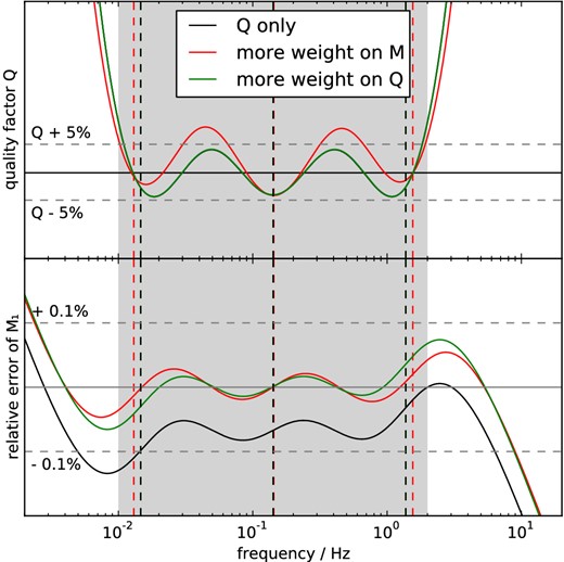
Optimized constant Q ≈ 250 (black) versus simultaneous optimization of Q and real part of the modulus M1 (red + green) using the relation by Kjartansson (1979) for a medium with three absorption bands: additional optimization of the modulus makes the parametrization independent of the choice of the reference frequency (here: fr = 2 Hz) and allows for tuning the parametrization towards lower phase errors at the boundaries of the frequency range (red) or lower amplitude errors (green). Vertical dashed lines indicate the relaxation frequencies ωj. Frequency weighting was not used for clarity.
2.3 Determination of the optimal structural parameters in full-scale applications
In full seismic applications, the material parameters aj and ωj need to be determined for many values of Q and seismic velocities, typically for each spatial gridpoint, that is, 106−109 times. The performance of an algorithm to find them is thus important and several approaches have been suggested.
This was proposed by Emmerich & Korn (1987) and later became more popular as the ‘τ-method’ by Blanch et al. (1995). The advantage of this method is that it results in only one inverse problem while finding the parameters for different Q is trivial due to the linearity of aj in Q−1. For low values of Q, this approximation introduces a logarithmic error to the resulting approximation of constant Q, see blue curve in Fig. 7(a). The largest error shows up at the high-frequency end of the frequency range of interest, that is, where the wavefield is most sensitive to such errors, see earlier. Furthermore, this problem becomes more dominant with increasing bandwidth.
![Recursive correction for the coefficients yj as in eq. (24): (a) linearization of Q in yj as suggested by Blanch et al. (1995; ‘τ-method’) leads to a logarithmic trend with the strongest effect in the high frequencies (blue), the correction (red) results in a behaviour very close to optimizing the exact relation (black) even for Q as low as 20 [on the global scale, the minimum value is ≈50 in the 3-D model QRLW8 by Gung & Romanowicz (2004)]. Errors are frequency-weighted, see text for details. (b) Frequency-weighted log-l2 error in Q as a function of Q for the linearization (dashed), the correction (solid) and the exact (dotted) relation.](https://oup.silverchair-cdn.com/oup/backfile/Content_public/Journal/gji/199/2/10.1093/gji/ggu314/3/m_ggu314fig7.jpeg?Expires=1716451074&Signature=UrQthTX4gJvMcFJyFALX6L2lJ-SOeE4fjsKudWr76JmWtuPdVApIeh5CoJCYXFfEPcGMijBn5BluQpsy4aOywrudzgx8W0GrwBPrSt-3jqCn4Hoi6nA4p2JZSFcRLrsNcpZnvY9nQ0eZqqX~~4Se0C3h6yTqysFyHZnqLqw9zP2wn0QkYYVgi~uBMGIrvibGO3BA~RYAx9AkD~NO4nUn7pD591Ig0Tg3IWuEf-orL~hVKnGpHmHF3dDtO-XGdIeTUO35pw4cG5bFTZ2kjhbC8qhlCk~VB2LR-WkgjpfLVZqXeERPUmm~l2Uk9JqxKZGchY9XjT2gMNRqIviHO8eXZQ__&Key-Pair-Id=APKAIE5G5CRDK6RD3PGA)
Recursive correction for the coefficients yj as in eq. (24): (a) linearization of Q in yj as suggested by Blanch et al. (1995; ‘τ-method’) leads to a logarithmic trend with the strongest effect in the high frequencies (blue), the correction (red) results in a behaviour very close to optimizing the exact relation (black) even for Q as low as 20 [on the global scale, the minimum value is ≈50 in the 3-D model QRLW8 by Gung & Romanowicz (2004)]. Errors are frequency-weighted, see text for details. (b) Frequency-weighted log-l2 error in Q as a function of Q for the linearization (dashed), the correction (solid) and the exact (dotted) relation.
Often, the relaxation frequencies ωj are not inverted for, but fixed log-spaced, since this allows for a linear (hence faster) inversion for the parameters aj as suggested by Emmerich & Korn (1987) by rearranging terms in eq. (7).
Similarly, Savage et al. (2010) use log-spaced frequencies, but a simplex approach for the non-linear inversion and suggest to use a look-up table to solve fewer inverse problems. However, these methods cannot handle the constraint aj > 0.
Liu & Archuleta (2006) present empirical formulae to interpolate the parameters between the largest and smallest value of Q in the model and use a simulated annealing approach to solve the remaining two inverse problems. As they do not present a closed form to find the coefficients in their interpolation, their formulae can only be used for their specific setup of frequency range, number of absorption bands N and Q range.
Here, we suggest a correction to the linearization as an easy-to-implement and computationally light method, combining the advantages of the linearization (‘τ-method’) with increased accuracy for low Q. As this results in a single inverse problem, the relatively expensive simulated annealing method can be used allowing to invert for the relaxation frequencies as well as including the constraint aj > 0.
The performance of this correction is visualized in Fig. 7, where panel (a) compares Q computed using corrected parameters to the linearization and the exact result for Q = 20. While the linearization causes an error of almost 20 per cent in the high frequencies, the corrected version is still quite close to the optimal solution using the exact relation. Fig. 7(b) shows tests of the approximation as a function of Q for a variety of different bandwidths and numbers of absorption bands in terms of the frequency weighted log-l2 error as defined earlier. The more accurate the approximation of constant Q is desired, the higher the Q value where the linearization breaks down: for example, at 2.2 decades bandwidth and using three absorption bands (red), the linearization (dashed) doubles the error for Q values lower than 90, while the corrected ones hit this error bound only for Q < 10. On the global scale, where Q typically takes values larger than 50, this scheme allows to find the parameters aj efficiently with very high accuracy.
This correction scheme has negligible computational imprint such that it may be used in the time loop, which means that the 2N coefficients aj and wj need to be stored only once and not for each gridpoint.
2.4 Analytic time stepping
Many discrete schemes have been proposed to integrate the memory variable equation, eq. (5), over time to determine the values of the memory variables at the next time step: for example, finite differences (Day & Minster 1984), some unspecified second-order scheme (Emmerich & Korn 1987), second-order central difference (Kristek & Moczo 2003), ADER (Käser et al.2007) or fourth-order Runge–Kutta (Komatitsch & Tromp 2002a; Savage et al.2010). To our best knowledge, integrating the equation analytically has not been published in the seismological community.
2.5 Generalization to three dimensions
Generalization to three dimensions is rather straightforward and extensive literature is available, for example, Carcione (2007) and references therein. We restrict ourselves to slightly anisotropic media, where the effect of attenuation can still be treated as isotropic and the anisotropy of attenuation is neglected as a second-order effect. In this case, the eigenstrains and eigenstiffnesses are easy to find as dilation and shear stresses and the stress–strain relationship remains simple and computationally light, see for example, Carcione & Cavallini (1994). The validity of this approximation for global radial anisotropy as in PREM is verified by the benchmark in Section 5.
Importantly, using the scheme from above to find the medium parameters, ωj are the same for bulk and shear Q, while the aj are found depending on the actual value of Qκ and Qμ. Identifying the right-hand side with s(t) from eq. (25), the analytical time stepping can readily be used in three dimensions.
3 AxiSEM DISCRETIZATION
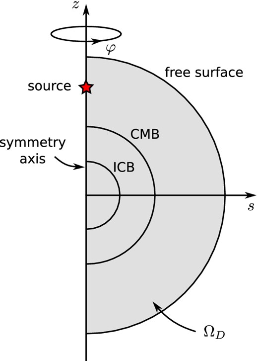
The cylindrical coordinate system (s, φ, z) and the reduced semi-circular 2-D domain ΩD for global wave propagation in axisymmetric media.
3.1 Angular dependence and axial boundary conditions of the memory variables
3.2 Anelastic stiffness terms in the weak form
3.3 Spectral element discretization
The next step is to generalize the spatial discretization of the stiffness terms from the anisotropic elastic case presented in van Driel & Nissen-Meyer (2014) to the anelastic case. The approach is the same as in the isotropic elastic case and we refer the reader to section in Nissen-Meyer et al. (2007b) for details and restrict ourselves to a short summary of the method and important aspects of the notation in the interest of brevity. A more general and rigorous approach can be found in Bernardi et al. (1999).
Here |$\delta _{{e}{\bar{e}}}$| is 1 in axial elements and 0 in all others and ζ0 is the vector of memory variables at the axis (i = 0). Equivalent terms for dipole and quadrupole case can be found in Appendix B.
Definitions for pre-computable matrices (i.e. prior to the costly time extrapolation) of the anelastic stiffness terms, ± takes its value depending on the combination of xζ as in the right-hand table. Subscript reference coordinates denotes partial derivation, for example, xζ = ∂ζx. For consistency with the summation notation in Nissen-Meyer et al. (2007a), we use indices i, j and I, J, which all take the values in {0…Ngll}.
| Matrix | Non-axial elements | Axial elements (i > 0) | (i = 0) | Axial vectors | |
|---|---|---|---|---|---|
| |$ ( { {\bf V}}_{x_\zeta } )^{ij}$| | |$\pm \sigma _i \sigma _j x_\zeta ^{ij} s^{ij}$| | |$\pm \bar{\sigma }_i \sigma _j (1 + \bar{\xi }_i )^{-1} x_\zeta ^{ij} s^{ij}$| | 0 | |$ ( { {\bf V}}^0_{x_\zeta } )^j = \pm \bar{\sigma }_0 \sigma _j x_\zeta ^{0j} s_\xi ^{0j}$| | |
| |$( { {\bf Y}} )^{ij}$| | |$\sigma _i\sigma _j {\mathcal {J}}^{ij}$| | |$\bar{\sigma }_i \sigma _j (1+ \bar{\xi }_i)^{-1}{\mathcal {J}}^{ij}$| | 0 | |$ ( { {\bf Y}}^0 )^j = \bar{\sigma }_0 \sigma _j {\mathcal {J}}^{0j}$| | |
| |$ ( { {\bf D}}_\xi )^{Ii}$| | ∂ξlI(ξi) | |$\partial _\xi \bar{l}_I(\bar{\xi }_i)$| | |$\partial _\xi \bar{l}_I(\bar{\xi }_0)$| | |$( { {\bf D}}_\xi ^0 )^{I} = \partial _\xi \bar{l}_I(\bar{\xi }_0)$| | |
| |$ ( { {\bf D}}_{\eta } )^{Jj}$| | ∂ηlJ(ηj) = ∂ξlJ(ξj) | ∂ηlJ(ηj) | |||
| | $\matrix{ \pm(x_{\zeta}) \qquad \zeta =\xi \qquad \zeta=\eta \\ x=s \qquad + \qquad\;\; - \\ x=z \qquad - \qquad\;\; + }$| | |||||
4 COARSE-GRAINED MEMORY VARIABLES
with the reference frequency ωr that should be within the frequency band of interest and the modulus at this frequency Mr, that is, δM(ωr) = 0 (see Fig. 9 for a schematic sketch). This choice of reference is equivalent to the ‘element-specific modulus’ by Graves & Day (2003), that is, the unrelaxed modulus that is used for the elastic stiffness is not the reference and will hence be not constant over the element. The idea of coarse grained attenuation then is to find a medium where δM is a function of space with the constraints (1) that it behaves macroscopically as the homogeneous medium and (2) reduces the numerical burden. This calls for a method to compute the macroscopic behaviour of a medium with structure on the subwavelength scale where the deviations are relative small in amplitude.
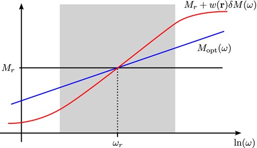
Coarse-grained attenuation schematically: constant Q corresponds to Mopt(ω). The problem is to find δM(ω) using standard linear solids for the anelastic GLL points. The constraint is that averaged with the elastic GLL points with modulus M0, the medium should behave as Mopt(ω) in the frequency range of interest (shaded in grey).
In a seminal paper, Backus (1962) showed how to average a layered medium to find a homogeneous long-wavelength equivalent medium. A similar argument was introduced in the context of heterogeneous finite-difference methods by Boore (1972) and further developed by Zahradnik et al. (1993) and Moczo et al. (2002). In more recent developments of homogenization theory (e.g. Capdeville et al.2010; Guillot et al.2010), more rigorous analytical arguments are raised and in the 1-D case, it can be shown analytically that the correct way of averaging the modulus is the harmonic average (Cioranescu & Donato 1999). Graves & Day (2003) show that harmonic averaging also yields better results than arithmetic averaging in the context of the coarse-grained memory variables in the case of small values of Q < 20 (where δM is relatively large) and yields the same results as arithmetic averaging if Q > 20. Although Q is larger than 50 for most global models, it is not obvious to generalize this conclusion to global body waves, because the test cases presented by Graves & Day (2003) are dealing with an order of magnitude-less wavelengths propagation distance (compare Section 2.2). We thus consider arithmetic averaging at first because of its simplicity and benchmark it in the next section, finding that it does suffice for global high-frequency body waves.
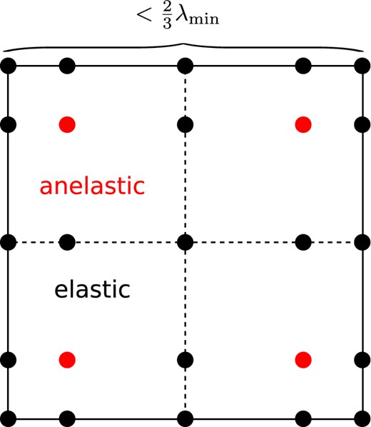
Distribution of Gauss–Lobatto–Legendre (GLL) integration points in the reference element of the fourth-order scheme. For the coarse-grained attenuation, anelasticity is concentrated on the four red GLL points, while the black points are treated as elastic. During meshing, element sizes are chosen to be smaller than |$\frac{2}{3}$| of the smallest wavelength, so that there are at least three anelastic points per wavelength.
The choice of GLL points is guided by the criterion derived by Day (1998), stating that the periodicity of the medium should have smaller scale than half the shortest wavelength to be propagated, that is, the elastic equivalent of the Bragg condition for normal incidence. In the specific case of five GLL points per element in each dimension that are meshed with |$\frac{2}{3} \lambda _s$| as element size, this leads to the choice of two anelastic points per element in each dimension. In principle, the dissipation mechanisms for the lower absorption bands could be placed even sparser, as they only affect longer wavelengths. While this would reduce memory usage and computational complexity in time stepping of the memory variables, we chose not to do so for simplicity in implementation and the fact that the stiffness term |${ {{\zeta }}}$| would end up less sparse if another distribution was chosen. Also, additional source terms for the memory variables would cause extra cost, as the strain is no field variable in our scheme. This might be different depending on the numerical scheme used: if the strain is a field variable and does not require extra computation, the decision might be different.
4.1 Numerical efficiency
The performance can benefit from the coarse grained implementation in multiple ways: The number of memory variables per element is smaller, so these use less memory. Also, the number of memory variable equations that need to be integrated in time and hence the number of points at which the source s(t) of these equations needs to be computed is less. The pre-computed matrices for the anelastic stiffness need only be computed and stored for the elastic GLL points. On top of that, the sparsity of |${{ {\zeta }}}$| can be exploited by using sparse implementations of the matrix products ⊗ and ⊙.
The observed performance gains in AxiSEM are summarized in Tables 2 and 3, showing roughly a factor of 2 in total memory reduction and a factor of 5 in computational time both for anelastic stiffness and memory variable time stepping, resulting in a total simulation speedup of around two. The additional cost of the anelastic terms compared to the elastic ones hence reduces from 150–200 per cent to 35–45 per cent for the Newmark time scheme. The ideal value for the speedup in anelastic stiffness and memory variable time stepping would be |$\frac{25}{4} = 6.25$|. In a full 3-D code, the dimensionality would increase this to |$\frac{125}{8} \approx 16$|. The anelastic addition to the elastic stiffness term in current implementations accounts for about 2/3 of the total runtime, and would then be diminished to the point where the elastic stiffness terms always dominate the computational cost.
Memory usage relative to the elastic case in terms of a multiplicative factor (Newmark time integration).
| N | Full memory variables | Coarse grained |
|---|---|---|
| 3 | 1.7 | 1.1 |
| 4 | 1.8 | 1.1 |
| 5 | 1.9 | 1.1 |
| 6 | 2.0 | 1.1 |
| 7 | 2.2 | 1.2 |
| 8 | 2.3 | 1.2 |
| N | Full memory variables | Coarse grained |
|---|---|---|
| 3 | 1.7 | 1.1 |
| 4 | 1.8 | 1.1 |
| 5 | 1.9 | 1.1 |
| 6 | 2.0 | 1.1 |
| 7 | 2.2 | 1.2 |
| 8 | 2.3 | 1.2 |
Computation time relative to elastic case in terms of a multiplicative factor (Newmark time integration).
| Elastic | Full memory variables | Coarse-grained | Total | Anelastic stiffness | Anelastic time step | |
|---|---|---|---|---|---|---|
| N | runtime | runtime | runtime | speedup | speedup | speedup |
| 3 | 1 | 2.55 | 1.35 | 1.9 | 5.3 | 4.3 |
| 4 | 1 | 2.75 | 1.38 | 2.0 | 5.2 | 4.5 |
| 5 | 1 | 3.0 | 1.41 | 2.1 | 5.3 | 4.7 |
| 6 | 1 | 3.16 | 1.44 | 2.2 | 5.5 | 4.7 |
5 BENCHMARK
Solving the full 3-D wave equation for arbitrary earthquake sources in axisymmetric anisotropic models, AxiSEM seems to be unique among available codes. For benchmarking we thus revert to spherically symmetric models. As a reference, we use Yspec by Al-Attar & Woodhouse (2008), which is a generalization of the direct radial integration method (Friederich & Dalkolmo 1995) including self-gravitation (switched off for the benchmark).
While Nissen-Meyer et al. (2008) could only perform benchmarks down to 20 s period due to limitations in the reference normal mode solution, this limit is overcome using Yspec. Also, AxiSEM since then has experienced some substantial development (Nissen-Meyer et al.2014), specifically the improved parallelization allows us to perform production runs up to the highest frequencies observed for global body waves.
Fig. 11 shows a record section of seismograms computed for the anisotropic PREM model (Dziewonski & Anderson 1981) with continental crust computed with Yspec and AxiSEM. The source is a normal faulting event with a moment magnitude Mw = 5.0 in 117 km depth under the Tonga islands. The traces recorded at some selected GSN stations are filtered between 10 and 1 s period. Due to the high-frequency content, it is necessary to zoom in to see any differences at all: the agreement between the two methods is remarkable even though the highest frequencies have travelled more than 1000 wavelengths (given the low-pass filter at 1 s, the time axis is equivalent to the number of travelled wavelengths).
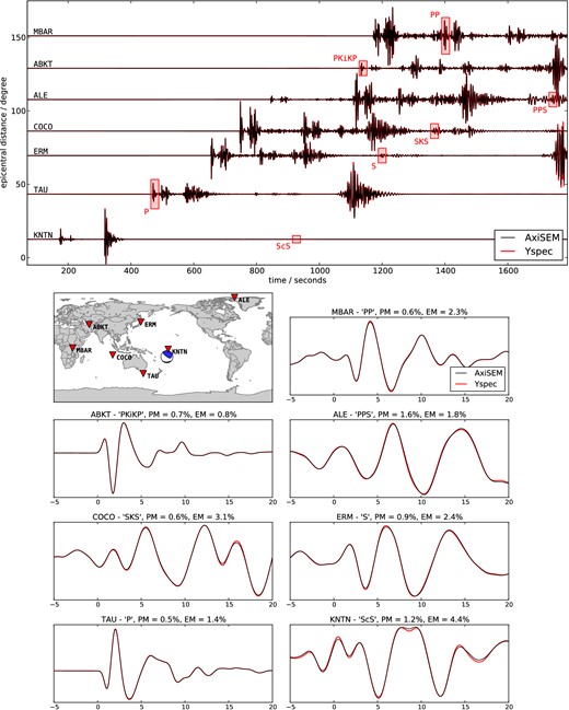
Comparison of vertical displacement seismograms (bandpass filtered from 10 to 1 s period) for a moment magnitude Mw = 5.0 event in 126 km depth under the Tonga islands, computed with AxiSEM and Yspec in the anisotropic PREM model without ocean but including attenuation. The traces are recorded at the GSN stations indicated in the map. The zoom windows are indicated with red rectangles in the record section and the timescale is relative to the ray-theoretical arrival. EM and PM denote the envelope and phase misfit in the time window plotted (Kristekova et al.2009). The largest envelope error is 4.4 per cent for the small amplitude phase ScS at KNTN.
We use the phase and envelope misfit PM and EM as defined by Kristekova et al. (2009) for quantitative comparison within the zoom windows and find phase misfits below 1.6 per cent for all windows and envelope misfits below 3.1 per cent for all windows but the extremely small amplitude phase ScS at KNTN, where it reaches a maximum of 4.4 per cent. These differences between AxiSEM and Yspec are slightly larger than in the purely elastic case (van Driel & Nissen-Meyer 2014), which is not surprising for a number of reasons: While Q is approximated using standard linear solids in AxiSEM, Yspec uses exactly logarithmic dispersion. The symplectic time scheme was developed for conservative systems (Nissen-Meyer et al.2008), while here the attenuation causes a slight energy loss. Also, the coarse-grained memory variable approach was implemented using arithmetic averaging instead of harmonic averaging and we neglected attenuation in the fluid outer core. Errors in amplitude and phase are therefore negligibly small compared to other errors when comparing these synthetics to data like, for example, noise or the assumption of a 1-D model.
The total cost of this extreme case, demanding run over 1800 travelled wavelengths at very high accuracy with AxiSEM was about 88K CPU hours on 11 048 cores [four simultaneous parallel jobs according to the decomposition described by Nissen-Meyer et al. (2007a)] using a fourth-order symplectic time scheme and five relaxation frequencies on a Cray XE6. The mesh was built for periods down to 0.8 s and the time step chosen 30 per cent below the CFL criterion, as this run was meant to prove convergence to the same result as Yspec. In applications where less accuracy is necessary one could either use the same traces at higher frequencies or reduce this cost substantially by choosing a larger time step and a coarser mesh (for instance, a dominant period of 1.6 s at otherwise fixed parameters is already an order of magnitude cheaper to compute due to the scaling with the third power of the period).
The additional cost for attenuation using the fourth-order symplectic time scheme and coarse-grained memory variables compared to a purely elastic simulation was only 26 per cent.
6 CONCLUSION AND OUTLOOK
In this paper, we presented three improvements for more efficient implementation of attenuation in time-domain wave-propagation methods. First, we showed how to find the optimal set of medium parameters to minimize errors in the wavefield at a fixed numerical complexity. To do so, we analysed first-order effects of errors in this parametrization onto the wavefield. Also, we derived an approximate method to find these parameters in a full-scale application, that is, for 106 or more different values of Q and the modulu. Furthermore, we suggested an analytical time-stepping scheme, that ties the error of the anelastic time integration to that of the global scheme. These findings are completely independent of the spatial scheme.
Finally, we generalized the coarse-grained memory variable approach to the spectral element scheme, noting that the same method could be used in other high-order finite-element schemes. This is a physical approximation reducing the cost of attenuation by a factor of 5 in the 2-D case of AxiSEM. Future work includes implementation of the coarse-grained scheme into high-order 3-D methods including homogeneous averaging for lower Q values.
We thank Paul Cupillard and an anonymous reviewer as well as the editor who helped to substantially improve this manuscript. We gratefully acknowledge support from the European Commission (Marie Curie Actions, ITN QUEST, www.quest-itn.org). Andreas Fichtner provided a basic version of the simulated annealing code. Data processing was done with extensive use of the ‘ObsPy’ toolkit (Beyreuther et al.2010; Megies et al.2011). Computations where performed at the ETH central HPC cluster (Brutus), the Swiss National Supercomputing Center (CSCS) and the UK National Supercomputing Service (HECToR), whose support is gratefully acknowledged.
