


Abstract
We present an analysis of the Mw = 5.3 earthquake that occurred in the Southeast Indian Ridge on 2010 February 11 using USArray data. The epicentre of this event is antipodal to the USArray, providing us with an opportunity to observe in details the antipodal focusing of seismic waves in space and time. We compare the observed signals with synthetic seismograms computed for a spherically symmetric earth model (PREM). A beamforming analysis is performed over the different seismic phases detected at antipodal distances. Direct spatial snapshots of the signals and the beamforming results show that the focusing is well predicted for the first P-wave phases such as PKP or PP. However, converted phases (SKSP, PPS) show a deviation of the energy focusing to the south, likely caused by the Earth's heterogeneity. Focusing of multiple S-wave phases strongly deteriorates and is barely observable.
1 INTRODUCTION
Focusing of seismic waves at the antipode of a seismic source has been attracting the attention of seismologists for many reasons. In antipodal regions, seismic phases propagating trough the inner core can be observed, providing information about the structure of this deepest part of the Earth (e.g. Butler et al.1986; Sun & Song 2002; Niu & Chen 2008). Antipodal energy focusing is also believed to play an important role during planetary-scale impacts (e.g. Meschede et al.2011). One can thus consider the antipode as a ‘collector’ of seismic-wave information (Rial 1978) where the waves propagating along different paths from all possible directions meet. At the antipode the waves concentrate and interfere, containing a global view of the Earth in a reduced area.
With modern numerical methods, the antipodal focusing of seismic waves can be studied theoretically in spherically symmetrical and heterogeneous Earth's models (e.g. Meschede et al.2011). In contrast, only very few observations of seismic signals recorded at antipodes of real earthquakes have been reported (e.g. Rial 1978; Rial & Cormier 1980; Poupinet et al.1993; Sun & Song 2002; Cormier & Stroujkova 2005; Niu & Chen 2008; Butler & Tsuboi 2010). Furthermore, quantifying the wave-focusing requires comparing observations at several stations located close to the antipode but at different distances from it. Lin & Tsai (2013) showed observation of the waves amplification at the antipode using waveforms reconstructed from seismic noise cross correlation methods.
Rial & Cormier (1980) used records at four stations, with epicentral distances ranging from 166.03° to 179.25°, to observe a clear antipodal amplification of different P phases (except the direct PKIKP wave). The observed waveforms, including their amplitudes, were found to be very similar to synthetic seismograms computed in spherically symmetrical earth models at the same set of epicentral distances. However, the small number of stations used did not allow these authors to investigate the details of the wave focusing in space.
In this study, we use a Mw 5.3 earthquake that occurred in the Southeast Indian ridge on 2010 February 11. The epicentre of this event was antipodal to the position of the Transportable Array (TA) component of the USArray (Fig. 1a). Therefore, the records of this earthquake by the TA stations provide us with a dense sampling of an antipodal wavefield over an extended area. We use instantaneous spatial snapshots of the observed wavefield and beamforming analysis to study the details of the spatial focusing of different seismic phases. The observations are compared with synthetic seismograms computed in the spherically symmetric earth model PREM (Dziewonski & Anderson 1981) in a period band between 20 and 50 s.
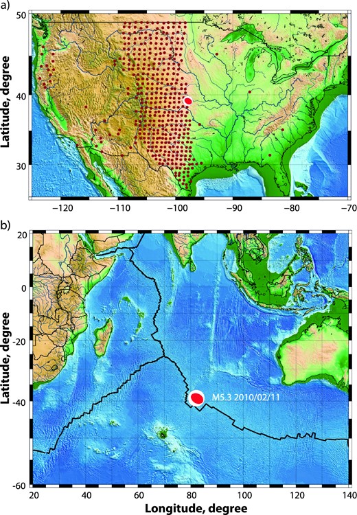
(a) Locations of USArray transportable array stations at the time of study with the location of the earthquake antipode. (b) Location and focal mechanism of the studied earthquake. Black lines indicate Indian Ocean ridges.
2 DATA
The earthquake of 2010 February 11 occurred in the Indian Ocean east of Amsterdam and St Paul Islands and had a magnitude Mw of 5.3. The earthquake's epicentre was located about 300 km off the Southeast Indian ridge (Fig. 1b) and was antipodal to the region where the USArray transportable network component was operating at that time (Fig. 1a). The moment tensor solution obtained from the global CMT project (Dziewonski & Anderson 1981; Ekström et al.2012) indicates a thrust faulting mechanism with a strong non-double-couple component (Fig. 1). Such mechanism is unusual for a mid-ocenic ridge environment and there is a possibility that it was not well resolved because of the poor station coverage in the southern hemisphere. At the same time, this intraplate event did not occur exactly at the ridge, which might explain the unusual mechanism. For the trust-fault event, all antipodal rays are concentrated near the maximum of the P-wave radiation pattern. We use the records from 411 stations of the USArray. All seismograms were corrected for instrumental responses and filtered with a Butterworth band pass filter between 20 and 50 s. Only the vertical component seismograms are used in this study.
3 ANTIPODAL AMPLIFICATION
Several phases may be detected at the antipode of an earthquake, having travelled through the mantle and core, as shown in Figs 2(a) and 3. Several phases are clearly observable in Fig. 3, where the signals of the three stations closets to the antipode are plotted. PKP (PKPab), PP, PcPPKP, PPP, SKSP and PPS show a strong signal-to-noise ratio. PKIKP (PKPdf) does not benefit from the amplification and thus is not clearly observable. However, the waveforms at the time of the PKIKP arrival are in phase indicating the signals from tele seismic waves and not a local noise.
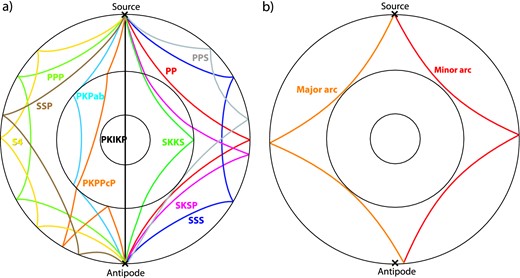
(a) Different seismic phases reaching the antipode of an earthquake. The phases travel through all the azimuth of the Earth. Paths were obtained using TauP path calculator (Crotwell et al.1999) based on the method of Buland & Chapman (1983). (b) Travel paths of the major and minor arc of a phase (here PP).
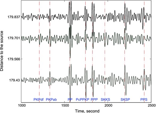
Vertical component seismograms of the three stations closest to the antipode of the event bandpassed between 20 and 50.
Except for PKIKP (PKPdf), which travels directly through the crust, mantle and core without any reflection or refraction and arrives at the antipode as an approximately plane wave, all the phases exhibit clear antipodal amplification resulting from the coherent interference of the waves reaching the antipode from all the different azimuths.
To illustrate the antipodal amplification, we compare seismograms recorded at different epicentral distances (Figs 4a and 5a). The signals were averaged in different distance bins to increase the signal-to-noise ratio. For each distance bin between 166° and 180°, the signals are averaged over all azimuths to increase the coherent amplitudes due to the earthquake and reduce potential noise. This averaging also suppresses the azimuthal variability, which we do not study.
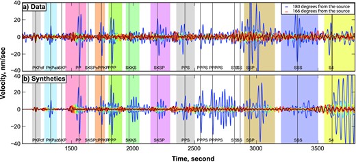
Vertical component seismograms bandpassed between 20 and 50 s and averaged in 1° distance bins. (a) Observations. (b) Synthetics. The colours of traces correspond to the distance from the source and evolve from red (166°) to blue (180°).
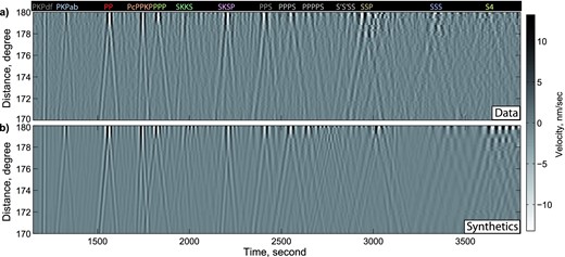
Time-distance gathers computed with averaging vertical-component seismograms in 0.25° bins. Signals were bandpassed between 20 and 50 s. (a) Observations. (b) Synthetics.
We then compare the observed signals with synthetic seismograms computed with AXISEM, a 2-D spectral-element solver for 3-D elastodynamics in global, spherically symmetric background models (Nissen-Meyer et al.2007), using the isotropic version of the PREM model (Dziewonski & Anderson 1981) and including viscoelastic attenuation. Results of this comparison are shown in Figs 4 and 5. The synthetics were computed using the global CMT focal mechanism and signals are generated at the same location as the USArray stations used and filtered in the same way as the USArray data, between 20 and 50 s. To focus on relative amplitudes between stations at different locations we normalized synthetics with a factor computed from amplitudes of the PP phase averaged over the five closest stations to the antipode. No time delay was applied. The signals are averaged over different distance bins similarly to the data (1° distance bins in Fig. 4 and 0.25° bins in Fig. 5)
Similarly to what is predicted from numerical modelling, the observed PKIKP waves arrive nearly simultaneously and with same amplitudes at all stations (Figs 4 and 5). This is explained by the incident angle of the waves arriving from under the network (Fig. 2a). A further study is shown in Appendix A.
For all other body-wave phases, the amplification is clearly observed. Observations over long-range of epicentral distances allows us to identify the converging and diverging branches propagating below minor and major arcs, respectively (Fig. 2b).
4 OBSERVATION OF SPATIAL FOCUSING
In Fig. 4, a considerable difference in the amplitudes between the observed and the synthetic antipodal signals appears after 2500 s when the wavefield begins to be dominated by seismic waves reflected many times at the surface, which are strongly sensitive to the upper-mantle structure. Amplitude of the observed seismic waves might be decreased because of (1) combination of a possible incomplete intrinsic attenuation and (2) the scattering at the 3-D heterogeneities, which are not considered in the synthetics. The effects of 3-D heterogeneities are more clearly revealed when analysing the spatial properties of the wavefield. Fig. 6 shows spatial snapshots of the observed and synthetic wavefields corresponding to times of maximum focusing (maximizing antipodal amplitude) of the different seismic phases: PKPab (PKP), PP, SKKS, SKSP, PPS and SSS.
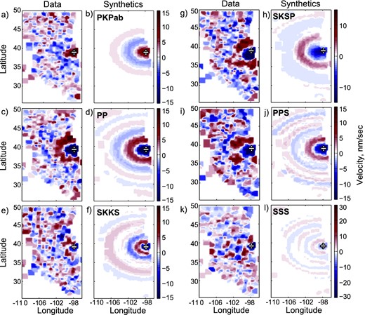
Spatial snapshots of the observed and synthetic velocity signals at the different stations at the time maximizing antipodal amplitude for PKPab, PP, SKKS, SKSP, PPS and SSS. We use the vertical component of the velocity signals bandpassed between 20 and 50 s.
These images are obtained by interpolating instantaneous values observed at individual stations at times of largest amplitude at the antipode for each phase. As a consequence, the signal-to-noise ratios are lower than those for stacked signals shown in Figs 4 and 5. Nevertheless, spatial patterns are clearly observed.
The observed patterns are compared to those obtained from synthetic seismograms computed with the source mechanism from the Global CMT catalogue. For the phases represented, the antipodal focusing results in interferometric patterns. When the waves are well focused, this pattern has a concentric structure with a main maximum coinciding with the position of the antipode as illustrated by predictions from synthetic seismograms (PKPab and PP phases in Figs 6a,b and 6c,d, respectively). Despite the low signal-to-noise ratios, clear interferometric patterns can be seen in the observations for most of P waves with the main maxima similar in size and position to those predicted for the spherically symmetrical Earth's model. In the best cases, a few secondary maxima can be recognized, as illustrated in Figs 6(c) and (d) for the PP phase. The patterns are quite consistent between the data and the synthetics with the same wavelength of the concentric circular structures and a focusing at the antipode.
The signal-to-noise ratio decreases for later arriving phases such as SKKS (Figs 6e and f). The observed interferometric patterns start to deviate from the predicted ones for the converted phases like SKSP or PPS (Figs 6g,h or 6i,j). The focusing deviates from the antipode and the patterns do not look circular anymore.
The observed interferometric patterns become strongly irregular and differ from the synthetic data for the multiply reflected S waves (Figs 6k and l), indicating that the 3-D heterogeneity deteriorates the focusing of these waves mainly propagating in the upper mantle.
5 BEAMFORMING ANALYSIS
Fig. 2 shows the ray paths for different phases focusing at the antipode. In a perfectly spherically symmetrical structure, waves arrive simultaneously from all directions and focus exactly at the antipode. As a consequence of the 3-D heterogeneity in the Earth, waves coming to the antipode from different directions do not arrive exactly simultaneously. These differences in traveltimes of waves coming from different directions distort the perfect focusing and, if sufficiently strong, may even shift the main focusing point away from antipode. Appendix B studies the possibility that this deviation is linked to the focal mechanism of the fault.
We apply a beamforming analysis to define the location of strongest focusing.
For this goal, we do not use the most standard ‘plane-wave’ beamformimg algorithm but a version where the traveltime shifts are computed with assuming a particular location of a focusing point.
The beamforming operator (1) formulated in frequency domain is equivalent to a sequence of three operations in time domain: (1) alignment of signals relative to a tested focal point, (2) shifting of signals assuming a constant slowness and (3) stacking. Application of the beamforming analysis to the PP waves is illustrated in Fig. 7. When we consider the antipode as a main focusing point (point 1 in Fig. 7e), the signals are well aligned and clearly show the minor and major waves (Fig. 7a). After applying time-shifts based on theoretical slowness of PP waves (Fig. 7b), converging waves arrive simultaneously and the resulting stack is very strong (Fig. 7e). When we test a position away from the antipode (Figs 7c and d, position 2 in Fig. 7e), the alignment and stacking are significantly deteriorated.
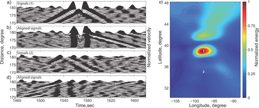
(a) Seismograms bandpassed between 20 and 50 s, stacked in 1° bins, and aligned with respect to distances to the epicentre's antipode. (b) Similar to (a) after applying a moveout correction with a slowness of PP waves propagating along the minor arc. (c) Similar to (a) but aligned with respect to point 2. (d) Similar to (c) and after applying a moveout correction maximizing the function from eq. (3). (e) Normalized beamforming result obtained from eq. (2) over an area around the antipode for the minor waves of PP. White numbers indicate positions of points 1 and 2 discussed in the text.
The geometry of the stations is not regular around the antipode of the earthquake with most of them located to the West (Fig. 1). This one-sided distribution may bias the shape of focusing determined with the beamforming analysis. To check this, we systematically tested the beamforming with a group of synthetic seismograms generated for stations homogeneously distributed around the antipode in addition to the analysis with real station locations (Appendix C). There results do not show significant variations compared to the results using the USArray locations.
6 DISCUSSION
Figs 8–13 show results of the beamforming analysis for several phases: PKPab, PP, SKKS, SKSP, PPS and SSS (see Fig. 2a for corresponding rays).
![Results of the beamforming for the phases PKPab. (a) Energy BR for the waves propagating along the minor arc and integrated in the slowness interval δs = [0.03 0.05] s km−1. The observations are represented as a colourmap and the synthetics with coloured lines. The energy is normalized for the synthetics and data separately for an easier comparison. The white cross shows the earthquake's antipode. (b) Energy BR for the waves propagating along the major arc (δs = [−0.05 −0.03] s km−1). (c) Energy Bs around main focusing locations δxδy (shown with the grey rectangles in a, b).](https://oup.silverchair-cdn.com/oup/backfile/Content_public/Journal/gji/199/2/10.1093/gji/ggu309/3/m_ggu309fig8.jpeg?Expires=1716441554&Signature=Gb27YKsvMiCOdAuY3k7gCgJBH6R1R8jJ0deWXjtUgfk5iU6SdxVAFK~JX4UhoNCOOePEP1Uv4K8sEATyY3H0GeSNjO3RhemO8-NhTop1RVV4GhkfZZpBcRP0NfvpnB5fo~H7tWfx-2aLkqhiaXKkm~gmsEnrXtQZY7-YA3Wy9PYbOVonH9JUpbr8tfU-dUgZO8i71ao9B91auLbTRSFRzzk~Vmqf6sAI-QelDG65n3V9BNQHl5qliloeu4tnQBLR6HBIYW3Y1thPil3161-rWOe5wlsM3mx1iBbEaZq5O6ns9nA-hM3BVwzyL~CfbP5lZaMxNPg0vovwpx6-usvDGw__&Key-Pair-Id=APKAIE5G5CRDK6RD3PGA)
Results of the beamforming for the phases PKPab. (a) Energy BR for the waves propagating along the minor arc and integrated in the slowness interval δs = [0.03 0.05] s km−1. The observations are represented as a colourmap and the synthetics with coloured lines. The energy is normalized for the synthetics and data separately for an easier comparison. The white cross shows the earthquake's antipode. (b) Energy BR for the waves propagating along the major arc (δs = [−0.05 −0.03] s km−1). (c) Energy Bs around main focusing locations δxδy (shown with the grey rectangles in a, b).
![Results of the beamforming for the phases PP. (a) Energy BR for the waves propagating along the minor arc and integrated in the slowness interval δs = [0.035 0.055] s km−1. The observations are represented as a colourmap and the synthetics with coloured lines. The energy is normalized for the synthetics and data separately for an easier comparison. The white cross shows the earthquake's antipode. (b) Energy BR for the waves propagating along the major arc (δs = [−0.055 −0.035] s km−1). (c) Energy Bs around main focusing locations δxδy (shown with the grey rectangles in a, b).](https://oup.silverchair-cdn.com/oup/backfile/Content_public/Journal/gji/199/2/10.1093/gji/ggu309/3/m_ggu309fig9.jpeg?Expires=1716441554&Signature=C0ZmFLKqUcMqUdt6CXYlDBOiNmkb7AimjlZIPtADfYHCFqIB~10s3o8H2Dmo49JkywNqIKaRV~ZpvpviN4ImJDTp~8O~vFSzZqxuwDBKP3qQuTlVgC5uk2lJo9ViPKowUWC8PqIjRwsqqe2xQ2jco7ChN5oNTh31EBvX5JAGqXKmlrr~4b8Hju4ohVAqt-zAKTEoh6v6t6IDrF6-E5D-fXUyy0SlAaKXYOV2vsb8PDTKB8i47PqcnM~3zU43-CR3Zzb5b3j4harMJCj~TJPLyK6jN9D-7c2r06uFaExaH0Ao1wQXOTvbrPLTIL-9Ci55YFQCpZcXMc0ZW1CdbkhhQQ__&Key-Pair-Id=APKAIE5G5CRDK6RD3PGA)
Results of the beamforming for the phases PP. (a) Energy BR for the waves propagating along the minor arc and integrated in the slowness interval δs = [0.035 0.055] s km−1. The observations are represented as a colourmap and the synthetics with coloured lines. The energy is normalized for the synthetics and data separately for an easier comparison. The white cross shows the earthquake's antipode. (b) Energy BR for the waves propagating along the major arc (δs = [−0.055 −0.035] s km−1). (c) Energy Bs around main focusing locations δxδy (shown with the grey rectangles in a, b).
![Results of the beamforming for the phases SKSP. (a) Energy BR for the waves propagating along the minor arc and integrated in the slowness interval δs = [0.035 0.065] s km−1 for the observations and δs = [0.025 0.05] s km−1 for the synthetics. The observations are represented as a colourmap and the synthetics with coloured lines. The energy is normalized for the synthetics and the data separately for an easier comparison. (b) Energy BR for the waves propagating along the major arc (δs = [−0.065 −0.035] s km−1 for the observations and δs = [−0.05 −0.025] s km−1 for the synthetics). (c) Energy Bs around main focusing locations δxδy (shown with the grey rectangles for the observations and orange rectangles for the synthetics in a, b).](https://oup.silverchair-cdn.com/oup/backfile/Content_public/Journal/gji/199/2/10.1093/gji/ggu309/3/m_ggu309fig10.jpeg?Expires=1716441554&Signature=s6k-SIZfgPsOorIuyfgqEvatIELdVXQuA95s9X9VBxIV32pR-2UxzpP7YjEbhPIPkvC~Vqo90d4xyGgwMFAhfsPOWm~H7JG2LMaHNpK4Hr7z9-22Ds5UfsQAWF-fdB2SkzijzncaEO0hYdfIzMGSwKcrqaqmnjVO1nJWtdkluU7bYhMUvOBg--fl8qts1n0M~rew5xgEd6-8K7ydAlrKN1xx6FN5gAhMEhTJf5FuR9NrJpVJnMzyJ6mMHV0V61Cj2yvbfw0STzCUHCAVNUT-VJh4AWtqVMh~36V7NiUL3r0-w6WGgv-sP2wBqpoBovf6FXUO2mqyBzyu63L-pmTiVg__&Key-Pair-Id=APKAIE5G5CRDK6RD3PGA)
Results of the beamforming for the phases SKSP. (a) Energy BR for the waves propagating along the minor arc and integrated in the slowness interval δs = [0.035 0.065] s km−1 for the observations and δs = [0.025 0.05] s km−1 for the synthetics. The observations are represented as a colourmap and the synthetics with coloured lines. The energy is normalized for the synthetics and the data separately for an easier comparison. (b) Energy BR for the waves propagating along the major arc (δs = [−0.065 −0.035] s km−1 for the observations and δs = [−0.05 −0.025] s km−1 for the synthetics). (c) Energy Bs around main focusing locations δxδy (shown with the grey rectangles for the observations and orange rectangles for the synthetics in a, b).
![Results of the beamforming for the phases PPS. (a) Energy BR for the waves propagating along the minor arc and integrated in the slowness interval δs = [0.045 0.075] s km−1 for the observations and δs = [0.05 0.08] s km−1 for the synthetics. The observations are represented as a colourmap and the synthetics with coloured lines. The energy is normalized for the synthetics and the data separately for an easier comparison. (b) Energy BR for the waves propagating along the major arc (δs = [−0.075 −0.045] s km−1 for the observations and δs = [−0.08 −0.05] s km−1 for the synthetics). (c) Energy Bs around main focusing locations δxδy (shown with the grey rectangles for the observations and orange rectangles for the synthetics in a, b).](https://oup.silverchair-cdn.com/oup/backfile/Content_public/Journal/gji/199/2/10.1093/gji/ggu309/3/m_ggu309fig11.jpeg?Expires=1716441554&Signature=dTVGSfU55HSKnFnFUvywPsDd973if8nuwosC~3LVP~IDAHLEuFhiKzTNA8vQwKiJsiMfkMxQyZ9Npx1v-C4Zc3-0ptjLXbAKEvMy-8VWZN92k-7F2y34rg5T74VrlvJ-GRZbD2mYSqXVhr4YrMOcGOFm-5JMn6bAdI4GDW-21uopxhcj08YqiH1pS0~Dqa70p33cqmd2tyzB5FXArWz7Kc3RK3lIjjOmO1ctb6ZBq9EX4Bmgabxvt2zG08TLx5IJOrFk-eZaLVlfhLIeyD2vjVSvk6YO~Xy99NHI2BUKDSVMXxgXcTXov-9PXXJWgSg8hE4B-qFTxOiS6WhvUeJ-Bw__&Key-Pair-Id=APKAIE5G5CRDK6RD3PGA)
Results of the beamforming for the phases PPS. (a) Energy BR for the waves propagating along the minor arc and integrated in the slowness interval δs = [0.045 0.075] s km−1 for the observations and δs = [0.05 0.08] s km−1 for the synthetics. The observations are represented as a colourmap and the synthetics with coloured lines. The energy is normalized for the synthetics and the data separately for an easier comparison. (b) Energy BR for the waves propagating along the major arc (δs = [−0.075 −0.045] s km−1 for the observations and δs = [−0.08 −0.05] s km−1 for the synthetics). (c) Energy Bs around main focusing locations δxδy (shown with the grey rectangles for the observations and orange rectangles for the synthetics in a, b).
![Results of the beamforming for the phases SKKS. (a) Energy BR for the waves propagating along the minor arc and integrated in the slowness interval δs = [0.02 0.05] s km−1 for the observations and synthetics. The observations are represented as a colourmap and the synthetics with coloured lines. The energy is normalized for the synthetics and the data separately for an easier comparison. (b) Energy BR for the waves propagating along the major arc (δs = [−0.05 −0.02] s km−1 for the observations and synthetics). (c) Energy Bs around main focusing locations δxδy (shown with the grey rectangles in a, b).](https://oup.silverchair-cdn.com/oup/backfile/Content_public/Journal/gji/199/2/10.1093/gji/ggu309/3/m_ggu309fig12.jpeg?Expires=1716441554&Signature=hXEvDa2l~q8p3PNFmIN526nhyOAFydpv503Cy8qexGfUsafdC57EhDR7wEIpH1P72pMoQANr8jN5s80GJE3J1jou~9uNf19Cujce-D87nF3uukvVz2whEH8uFgRTOE2UBq2S9b7iaqUwzDZNkdydmGcJP8RYy1k0pT1yKBFCp4GrNPSrbJdzGi6sbUHAZQ8lUlfORfCJnvcIUUYRbp9eAyroODvwKGFZ0VhSXe4IQdcO1WXBLzb0Mt5wwQNWuiRzP2rFV4SOGEqyWOPFEEmKxmSsDUa10DKETm5pkn12Zmqleqh8jJc2nm4as3Sk4OwtYLAxGl5LrNMxMqnMgTyuWQ__&Key-Pair-Id=APKAIE5G5CRDK6RD3PGA)
Results of the beamforming for the phases SKKS. (a) Energy BR for the waves propagating along the minor arc and integrated in the slowness interval δs = [0.02 0.05] s km−1 for the observations and synthetics. The observations are represented as a colourmap and the synthetics with coloured lines. The energy is normalized for the synthetics and the data separately for an easier comparison. (b) Energy BR for the waves propagating along the major arc (δs = [−0.05 −0.02] s km−1 for the observations and synthetics). (c) Energy Bs around main focusing locations δxδy (shown with the grey rectangles in a, b).
![Results of the beamforming for the phases SSS. (a) Energy BR for the waves propagating along the minor arc and integrated in the slowness interval δs = [0.095 0.145] s km−1 for the observations and δs = [0.105 0.15] s km−1 for the synthetics. The observations are represented as a colourmap and the synthetics with coloured lines. The energy is normalized for the synthetics and data separately for an easier comparison. (b) Energy BR for the waves propagating along the major arc (δs = [−0.145 −0.095] s km−1 for the observations and δs = [−0.15 −0.105] s km−1 for the synthetics). (c) Energy around main focusing locations δxδy (shown with the grey rectangles for the observations and orange rectangles for the synthetics in a, b).](https://oup.silverchair-cdn.com/oup/backfile/Content_public/Journal/gji/199/2/10.1093/gji/ggu309/3/m_ggu309fig13.jpeg?Expires=1716441554&Signature=dJZypvQR08Jknqzz92sJflgQvqbfWNovk~eYGMPqMA8Ez16zI09I9Vd2Uzf-QLEgioqCFQTj~yFOmOFmKhJJFnoMPMOft4grbHz9G3v~vRio4G6OAt2Pz4~YU-R1~3QaMo-kD5VdHNVCrFIwCDY9-XqqSdL2PEafO-M-anL2hKxgYrqDDD8GRMyXWUiQdN4eXdfWkWLH9qz93JMEItmIPTkT3xXIymxD0~sMUppG1juSmF1-cRWvwISXKw5US6Bbgl6GkMDn31g-nQ2dm3uz1goe~J15HeifAR9neI8Izo2chZZ2xcuGSN1kHX0rC5KEHCpdgHkTT54wSFNj4-5z9g__&Key-Pair-Id=APKAIE5G5CRDK6RD3PGA)
Results of the beamforming for the phases SSS. (a) Energy BR for the waves propagating along the minor arc and integrated in the slowness interval δs = [0.095 0.145] s km−1 for the observations and δs = [0.105 0.15] s km−1 for the synthetics. The observations are represented as a colourmap and the synthetics with coloured lines. The energy is normalized for the synthetics and data separately for an easier comparison. (b) Energy BR for the waves propagating along the major arc (δs = [−0.145 −0.095] s km−1 for the observations and δs = [−0.15 −0.105] s km−1 for the synthetics). (c) Energy around main focusing locations δxδy (shown with the grey rectangles for the observations and orange rectangles for the synthetics in a, b).
We observe a robust focusing for the main P-wave phase: PKPab (Figs 6a and 8) and PP (Figs 6c and 9), for both the minor and the major arc propagations (Fig. 2b).
The main observed focal spot is very close to the prediction from PREM in terms of its location and spatial extent for PP, the phase with highest amplitude. The energy of the PP waves is well focused at the antipode position (Fig. 9). The slowness observed at the antipode (after averaging over the main focalization zone) is of 0.045 s km−1 for the waves propagating along the minor arc and −0.045 for the ones propagating along the major arc (Fig. 9c) which is very close to predictions estimated by global traveltime tables (Buland & Chapman 1983). The main difference between the observations and the synthetics is the ratio of amplitude of the beamforming energy between the minor and major arc propagations. Similarly, the PKPab phase (Fig. 8) shows a good focusing at the antipode and a good match between the observed and the predicted major slownesses.
For the phase SKSP, the observed focusing significantly differs from the synthetic prediction. In the spatial snapshot representation and in the beamforming results (Figs 6g and 10a), a decay of about 115 km to the south is observed between the energy focusing of the observations and synthetics. The maximum slowness observed with the data is 0.05 s km−1, while the value predicted with synthetic seismograms is 0.035 s km−1. A similar southward shift of the main focusing position is observed for another converted phase PPS (Fig. 11). In contrast, the phase SKKS does not exhibit the southward shift of the main focusing location (Fig. 12) though it seems disturbed by the previous arrivals and shows a low signal-to-noise ratio (Fig. 4).
The observed focusing becomes very disturbed for the multiple S waves: SSP, SSS, SSSS … (Figs 6d and 13). The energy is still amplified when closer to the antipode, but the main focusing spot is badly defined for the data when compared with the synthetics. This observation confirms the strong influence of the upper mantle S velocity heterogeneity on the defocusing of the antipodal phases.
The southward shift of the main focus point that is not systematically observed in all phases is difficult to explain by an effect of focal mechanism. First, the mechanism from the Global CMT catalogue has a dip close to 45° and in this case the expected shifts are very small, as discussed in Appendix B. Nonetheless, a shift caused by a very different mechanism than the Global CMT mechanism should imply similar behaviour for all phases generated as P or as S waves at the source of the event. Even so, the shift is only observed for some phases and not for others. Therefore, the most likely explanation is that this shift is caused by some large-scale heterogeneity within the Earth.
The most important southward shift of the focus point is observed for the SKSP phase. However, PKPab and another S-wave phase, SKKS, which both travel through the core, do not exhibit the same systematic variation. They all travel through the core, but SKSP waves bounce one time at the surface, indicating that the heterogeneity is located in the mantle or the crust rather than in the core.
The first P-wave phases focus at the antipode and do not show this shift but there are deteriorations later in the signals. Indeed no shift is observed for PP and PKPPcP. However, PPP and PPS are shifted, meaning that shifts can be the consequence of multiple bounces.
These variations of focusing could be linked to the different travelpaths of the waves arriving at the antipode from the south or the north. Waves travelling to the antipode from the north bounce mostly in the continental crust of Eurasia, while waves travelling from south bounce mostly within the oceanic crust. The differences in crustal thickness or the differences of mantle and crust composition in oceanic or continental contexts might induce time delays or changes in the shapes of the waveforms, perhaps implying signal interference, changing the focusing of the waves.
We thank Matthieu Landes for fruitful discussions. We thank Alexandre Fournier and Tarje Nissen-Meyer for their help on the computing of synthetics with Axisem. Data from the TA network are made freely available as part of the EarthScope USArray facility, operated by Incorporated Research Institutions for Seismology (IRIS). This work was supported by the Commissariat l'Energie Atomique (CEA, France) and by the European Research Council under the contract FP7 ERC Advanced grant 227507 (WHISPER).
REFERENCES
APPENDIX A: OBSERVATION OF PKIKP BEHAVIOUR
Phase PKIKP shows a different behaviour from the other phases because of the arrival of the waves from right under the network (Fig. 2a). This implies that the waves arrive at the same time at the different stations of the network (Figs 4 and 5) and thus do not interfere into a focalization effect.
Spatial snapshots are performed to show this behaviour, using the same method as in Section 4. As expected, the amplitude of the PKIKP waves is constant over the whole network (Fig. A1) for the data and synthetics, showing the simultaneous arrivals of the PKIKP waves.
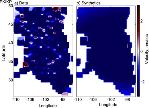
Spatial snapshots of the observed and synthetic velocity signals at the different stations at the time maximizing antipodal amplitude for PKIKP. We use the vertical component of the velocity signals bandpassed between 20 and 50 s.
Furthermore, beamforming analysis, discussed in Section 6, shows this effect too. No strong focusing is observed for the PKIKP wave (Fig. A2), which agrees with the simultaneous arrival time of the signal at all stations (seen on Figs 4 and 5). This behaviour is predicted by synthetic seismograms and is well seen in the data, despite the low signal-to- noise ratio (Fig. A1). The most efficient slowness obtained for this phase is around zero implying an almost vertical incidence of this wave at the antipode explained by its travelpath (Fig. 2a).
![Results of the beamforming for the phase PKIKP. (a) Energy BR integrated in the slowness interval δs = [−0.01 0.01] s km−1. The observations are represented as a colourmap and the synthetics with coloured lines. The energy is normalized for the synthetics and data separately for an easier comparison. The locations of the stations are represented with the black points. (b) The energy Bs computed over the all area since no focusing is observed.](https://oup.silverchair-cdn.com/oup/backfile/Content_public/Journal/gji/199/2/10.1093/gji/ggu309/3/m_ggu309figa2.jpeg?Expires=1716441554&Signature=Ys4HPUl-aH9W5COxbJt73Kd7HCerVHQmAM85Ny6LRxPpQxzgUuf1wqNa-~nrMcHuBCkKWZXIyaFEOWt72L5RgA9jPzR0bQs-h2NhgL3fFEYuRd3rr-e~saCroOcBtEGTT-aiJvfxCW8gcYKE6BnMpBnw5KVVrn1VFZIUCdn70vHhJwGJ-Ke~sD2hgZg-ymm79roWG-Tj6tTUu8boC3lncNbImKDTlwAhE36OqhYn6nxMYGh8Cns2w38g4JgWdDis~rfHfIIvuqqSuFajSxWz80H2Ld3NUvD4OZYz41sHvCiPLQCPqSlTh7Uo6H5y4~5OyvZmuay1wDffuD0oM-zwLA__&Key-Pair-Id=APKAIE5G5CRDK6RD3PGA)
Results of the beamforming for the phase PKIKP. (a) Energy BR integrated in the slowness interval δs = [−0.01 0.01] s km−1. The observations are represented as a colourmap and the synthetics with coloured lines. The energy is normalized for the synthetics and data separately for an easier comparison. The locations of the stations are represented with the black points. (b) The energy Bs computed over the all area since no focusing is observed.
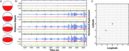
(a) The different tested focal mechanisms are plotted on the left-hand side of the figure. The strike and rake are constant with a value of 90°. The dip varies from 0° to 45° (by steps of 15°). (b) Synthetic displacement seismograms computed at near antipodal stations. The signals are filtered using a Butterworth bandpass filter between 20 and 50 s. The signals are drawn for three stations (plotted in c) at 175°, 177.5° and 180° of distance from the source (green, red and blue traces, respectively). (c) The different locations of the computed signals (175°, 177.5° and 180° in black, red and blue). Position (0,0) is the antipode of the source.
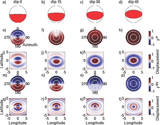
(a) The different focal mechanisms tested. The strike and rake are constant with a value of 90°. The dip varies from 0° to 45°. (b) Radiation patterns of the PP phase computed from (1) and shown in polar coordinates centred at the antipode position and distances varying between 174° and 180°. The white circles represent the distances to the source 175° and 177.5°. (c) Normalized vertical displacement for PP phase at the time of largest amplitude at the antipode at different positions. The magenta star shows the antipode location. (d) Radiation patterns of the SS phase computed from (2) and shown in polar coordinates centred at the antipode position and distances varying between 174° to 180°. (e) Amplitude displacement for SS phase at the time of largest amplitude at the antipode at the different positions.
![Results of the beamforming performed on synthetics for the phases PP. (a) Energy BR for the waves propagating along the minor arc and integrated in the slowness interval δs = [0.035 0.055] s km−1. The energy is normalized for the synthetics and data separately for an easier comparison. The white points show the location of the USArray station. (b) Energy BR for the waves propagating along the major arc (δs = [−0.055 −0.035] s km−1). (c, d) Beamforming results computed from synthetic seismograms with a homogeneous distribution of stations. The white points represent the location of the well distributed stations. (e) Energy Bs around main focusing locations δxδy (shown with the grey rectangles in a, b, c, d).](https://oup.silverchair-cdn.com/oup/backfile/Content_public/Journal/gji/199/2/10.1093/gji/ggu309/3/m_ggu309figa5.jpeg?Expires=1716441554&Signature=A57WA4YZbBXR71eXylYKofcAVgN1EEHJU30MpiC82UKkccJmcqY4A62HXbaXsFmee~~6CcThN7q3c3DERyXRw7Ga6bRxHGWUiET6YMwos~uZMu4fJim8h04JggEQb73WjYiMqc3Dxfa3QZeHL6F08dh5vd--TWyJubN1HmtXGj~RLNRGp~7NssdjKKbO4QJQ6RF8q48fvEfhCHhRNe7-lbA6-iq35-XbkO7KQx1oPLS20bm2f~2k5fwUY0V1I5JKDgmSmlC15Dr0CS3zMMMVV9-3TkdoAtyHSOCe0nKYfeSmSN-jXVlm1nZ0mxsjNstVlyPpdaYi8xVqOWbj3cywIg__&Key-Pair-Id=APKAIE5G5CRDK6RD3PGA)
Results of the beamforming performed on synthetics for the phases PP. (a) Energy BR for the waves propagating along the minor arc and integrated in the slowness interval δs = [0.035 0.055] s km−1. The energy is normalized for the synthetics and data separately for an easier comparison. The white points show the location of the USArray station. (b) Energy BR for the waves propagating along the major arc (δs = [−0.055 −0.035] s km−1). (c, d) Beamforming results computed from synthetic seismograms with a homogeneous distribution of stations. The white points represent the location of the well distributed stations. (e) Energy Bs around main focusing locations δxδy (shown with the grey rectangles in a, b, c, d).
![Results of the beamforming performed on the synthetics for the phases SKSP. (a) Energy BR for the waves propagating along the minor arc and integrated in the slowness interval δs = [0.025 0.05] s km−1. The observations are represented as a colourmap and the synthetics with coloured lines. The energy is normalized for the synthetics and data separately for an easier comparison. (b) Energy for the waves propagating along the major arc (δs = [−0.05 −0.025] s km−1). (c, d) Beamforming results computed from synthetic seismograms with a homogeneous distribution of stations. (e) Energy Bs around main focusing locations δxδy (shown with the grey rectangles in a, b, c, d).](https://oup.silverchair-cdn.com/oup/backfile/Content_public/Journal/gji/199/2/10.1093/gji/ggu309/3/m_ggu309figa6.jpeg?Expires=1716441554&Signature=Mxf0pzpOdenwY2fSzfFmcW8Fj1hc4emFFtcM3sq0F0PbrrIXHjbe926PWM2Dlwf9PnxnTIj0syIM3LkThR5TDdom94AroMX3t1ZM4rViQhULQZphqAZaJWN9F--4ysA560T7JiXR-JCmH6oX958YDSZUA0MkLY8iso0mvVP94NVH5HZAYJcnGK-yuxoHtnzL~LTQpzubnGq8RN-isNG160M8pTLTEWRAHV5oiR-xIfVD1eoGtqK6RjaaNYJDFct41rOUIjEj6fdGj95~mdKqrObD0O9NN85kst1H4JfrfAvTQhak0xEwHeo54Jh4aDoOtFCfDhno6n7Td43-BHrxjw__&Key-Pair-Id=APKAIE5G5CRDK6RD3PGA)
Results of the beamforming performed on the synthetics for the phases SKSP. (a) Energy BR for the waves propagating along the minor arc and integrated in the slowness interval δs = [0.025 0.05] s km−1. The observations are represented as a colourmap and the synthetics with coloured lines. The energy is normalized for the synthetics and data separately for an easier comparison. (b) Energy for the waves propagating along the major arc (δs = [−0.05 −0.025] s km−1). (c, d) Beamforming results computed from synthetic seismograms with a homogeneous distribution of stations. (e) Energy Bs around main focusing locations δxδy (shown with the grey rectangles in a, b, c, d).
PKIKP is the only phase showing this behaviour because it is the only one travelling directly from the source to the network with no refraction or reflection at the different interfaces of the earth. It gives a direct view of the event and the earth travelled without interferences between the arrivals.
APPENDIX B: INFLUENCE OF THE EARTHQUAKE FOCAL MECHANISM ON THE ANTIPODAL AMPLIFICATIONS
Antipodal amplification is due to constructive interferences of waves arriving at the antipode from different directions. This interference may be partially damaged if waves coming from different azimuth do not arrive exactly in phase. One possible cause for such decorrelation might be the influence of the 3-D heterogeneity within the Earth. Therefore, observing the deviation of the antipodal amplification and focusing from predictions in the spherically symmetric models could help quantify the degree of the Earth's heterogeneity. Another possible cause of non-perfect antipodal focusing might be the influence of the source radiation pattern.
The influence of focal mechanism was tested with synthetic seismograms. 625 synthetic signals are generated for virtual stations disposed uniformly around the antipode with distances from 174° to 180° to the source of the earthquake (Fig. A3c). The synthetics are filtered using a Butterworth bandpass filter between 20 and 50 s. Different earthquake mechanisms are tested (Figs A3a and b). The strike and rake are constant with a value of 90° while the dip varies from 0° to 45°. For mechanisms with nearly vertical or nearly horizontal fault planes, vertical-component seismograms have low amplitudes for both P and S waves at antipodal stations. The reason for this is that the antipode coincides with the minima of the P-waves radiation pattern while most of the radiated S-waves energy propagates along horizontal components. For such mechanisms, the maximum of energy is shifted from the antipode (Fig. A4).
To interpret the observation made on vertical components, we use the FP radiation pattern for P waves and FSV radiation pattern for S waves (eqs B1 and B2, respectively). These radiation patterns are compared with amplitudes predicted by synthetic seismograms in Fig. A4. For a 45° dip fault the antipodal energy focusing is predicted for both PP and SS waves. With the variation of the dip from 45° to 0°, the locations of apparent focal points shift away from the antipode. The directions of these shifts are opposite for P and S waves, which may lead to discrepancies in their maximum focusing positions.
APPENDIX C: BEAMFORMING RESULTS OBTAINED BY USING WELL DISTRIBUTED RECEIVERS
To observe the possible effect of the stations distribution in the beamforming results we performed the analysis explained in Section 6 on synthetics generated for a set of stations well-distributed around the antipode. Figs A5 and A6 give the results of the beamforming analysis for the synthetics generated at the location of USArray (a, b) and the synthetics generated using a set of well distributed stations around the antipode (c, d) for the phases PP and SKSP.
The results obtained with the beamforming method are similar when using synthetics generated with well-distributed stations or for the USArray locations. Still, some variations are observable, showing that the station distribution has some influence, but it does not influence the interpretations.
