Abstract
In recent years, the application of time-domain adjoint methods to improve large, complex underground tomographic models at the regional scale has led to new challenges for the numerical simulation of forward or adjoint elastic wave propagation problems. An important challenge is to design an efficient infinite-domain truncation method suitable for accurately truncating an infinite domain governed by the second-order elastic wave equation written in displacement and computed based on a finite-element (FE) method. In this paper, we make several steps towards this goal. First, we make the 2-D convolution formulation of the complex-frequency-shifted unsplit-field perfectly matched layer (CFS-UPML) derived in previous work more flexible by providing a new treatment to analytically remove singular parameters in the formulation. We also extend this new formulation to 3-D. Furthermore, we derive the auxiliary differential equation (ADE) form of CFS-UPML, which allows for extension to higher order time schemes and is easier to implement. Secondly, we rigorously derive the CFS-UPML formulation for time-domain adjoint elastic wave problems, which to our knowledge has never been done before. Thirdly, in the case of classical low-order FE methods, we show numerically that we achieve long-time stability for both forward and adjoint problems both for the convolution and the ADE formulations. In the case of higher order Legendre spectral-element methods, we show that weak numerical instabilities can appear in both formulations, in particular if very small mesh elements are present inside the absorbing layer, but we explain how these instabilities can be delayed as much as needed by using a stretching factor to reach numerical stability in practice for applications. Fourthly, in the case of adjoint problems with perfectly matched absorbing layers we introduce a computationally efficient boundary storage strategy by saving information along the interface between the CFS-UPML and the main domain only, thus avoiding the need to solve a backward wave propagation problem inside the CFS-UPML, which is known to be highly ill-posed. Finally, by providing several examples we show numerically that our formulation is efficient at absorbing acoustic waves for normal to near-grazing incident body waves as well as surface waves.
1 INTRODUCTION
Large-scale complex wave propagation problems in unbounded domains are frequently encountered in earthquake simulations, seismic tomography, geophysical exploration, ocean acoustics or non-destructive acoustic testing for instance. In the application of time-domain adjoint methods and imaging to improve our knowledge of large, complex underground tomographic models, it is important to model heterogeneous media accurately at the local and regional scale. In order to limit the computational cost of such iterative imaging problems or even very high frequency forward problems for a given model solved for instance based on a time-domain finite-element (FE) or finite-difference (FD) method, one aims at reducing the problem size by introducing efficient artificial absorbing boundaries to truncate the semi-infinite or infinite medium. In the case of convex artificial boundaries, one acceptable assumption that simplifies the setup of the truncated problem is that all waves leaving the truncated domain are purely outgoing and should thus never reenter it (Liao & Wong 1984). Along such artificial boundaries, infinite-domain truncating methods should thus be introduced to reduce or even eliminate the spurious boundary reflections, which is important in particular if thin mesh slices are used and/or if receivers are located at large offset (Martin & Komatitsch 2009).
Simple summation of different runs performed with Dirichlet (rigid) and then Neumann (free) totally reflecting boundary conditions, leading to cancellation of reflections with opposite sign was introduced by Smith (1974) but is not satisfactory because, while it is exact for reflections that occur in the corner of the model under study, it does not work for waves reflected off opposite model edges nor for multiple (high-order) corner reflections. In addition, such an approach is expensive because it requires summing eight runs in 3-D and four runs in 2-D; it has therefore been abandoned nowadays. Four main types of methods have been introduced since then (Givoli 2004), namely, boundary integral methods (BIMs), infinite element methods (IEMs), absorbing layer methods (ALMs) and absorbing boundary condition (ABC) methods, which can be further divided into global ABCs and local ABCs. BIM, IEM, together with global ABCs are only of limited application in the case of complex models due to the fact that: (i) they are valid only for homogeneous unbounded domains; (ii) they are valid only for a particular shape of the artificial boundary and (iii) their computational cost is often high. More details can be found for instance in Ting & Miksis (1986), Chen et al. (2004), Teng (2003) and Grote & Kirsch (2007) regarding BIM, Astley & Hamilton (2006) regarding IEM and Givoli & Keller (1990), Grote & Keller (1995), Keller & Grote (2000) and Givoli & Patlashenko (2004) regarding global ABCs. Thus, only local ABCs and ALMs are currently widely used.
The main idea behind the design of a local ABC is to use the outgoing nature of waves that need to be absorbed, which implies that the values on artificial boundaries can be extrapolated based upon past time values. Thus, in its continuous form before discretization by a numerical scheme, all spatial derivatives along the normal direction of an artificial boundary are one-sided. Since the end of the 1970s, different families of local ABCs have been developed, such as viscous boundary conditions (Lysmer & Kuhlemeyer 1969), viscous-spring boundary conditions (Deeks & Randolph 1994; Liu & Li 2005), paraxial conditions (Clayton & Engquist 1977; Stacey 1988), asymptotic operators (Bayliss & Turkel 1980), multitransmitting boundary conditions (Liao et al.1984) and Higdon boundary conditions (Higdon 1986, 1990). The first two are only of first order, while the other four families provide a hierarchy of local ABCs with increasing accuracy order. A long-standing problem in the application of a local ABC is that it is hard to construct stable numerical schemes for high-order local ABC due to the presence of high-degree one-sided normal derivatives. Furthermore, due to the difficulty in establishing the well-posedness of local ABC formulations, instabilities encountered in their implementation are not well understood nor solved. There is thus ongoing research work on that topic, and significant progress has been made in recent years. First, by reformulating paraxial conditions, Higdon boundary conditions or asymptotic operators (Guddati & Tassoulas 2000; Givoli & Neta 2003; Hagstrom & Warburton 2004; Hagstrom et al.2008; Hagstrom & Warburton 2009), the so-called practical high-order local ABCs have been proposed. In these conditions, high-degree normal derivatives are eliminated based on the use of auxiliary variables, defined only on the artificial boundary and assumed to satisfy the interior wave equation. Secondly, by adding a Lysmer–Kuhlemeyer operator inside the Higdon boundary conditions, a long-time stable high-order ABC has been derived and implemented for a 2-D elastic guided-wave problem by Baffet et al. (2012). However, for a layered infinite domain or even a homogeneous infinite domain governed by the second-order wave equation written in displacement, long-time stable high-order ABC formulations are still not available (Rabinovich et al.2011, 2013). Other stable implementations of high-order ABCs have been obtained from space–time localization of global ABCs (Alpert et al.2002; Du & Zhao 2010; Grote & Sim 2011), however these ABCs inherit the limitations of global ABCs. This is the reason why simple first-order ABCs are still widely used nowadays, but one needs to impose them sufficiently far from the region of interest in order to get relatively accurate results because their efficiency at absorbing waves is often relatively poor. Unfortunately, this is computationally inefficient.
In parallel, ALM is undergoing rapid development. The main idea of an ALM is to replace the infinite domain outside the artificial boundary with an absorbing layer of finite width. Thus, ideally on the artificial boundary waves can enter from the main domain into the absorbing layer without generating any reflection, and then damp out exponentially. ALM can be divided into two main groups: (i) sponge layers, which include the tapering absorbing layer (Cerjan et al.1985) and physical absorbing layers (Israeli & Orszag 1981; Kosloff & Kosloff 1986; Sochacki et al.1987; Sarma et al.1998; Semblat et al.2011); (ii) Perfectly matched layers (PML), the main advantage of PML over sponge layers being that in the continuous and infinite case waves enter into the absorbing layer without generating any reflection irrespective of their frequency and incidence angle (hence the name ‘perfectly matched’). For a PML of finite size, damped-out waves will reflect off the outer edge of the PML, on which a Dirichlet rigid condition, that is, a condition with total reflection is implemented, and will be damped again on their way back to the entrance of the PML; thus theoretically these waves are not zero, but their amplitude is damped by an exponential factor that depends on twice the thickness of the PML (since the waves travel through it twice) and thus in practice they are extremely small. Sponge layers are not perfectly matched, which makes their efficiency small in practice because significant spurious reflections occur. The use of smooth attenuation profiles can partially alleviate this difficulty, but doing so requires thick regions and consequently additional storage and computation. PML was originally developed by Bérenger (1994) in electromagnetism. Then, the interpretation and rederivation of PML in terms of complex-coordinate-stretching or complex-field-stretching methods (Chew & Weedon 1994; Teixeira & Chew 1998) led to its rapid development and application in other fields such as acoustics, elastodynamics, poroelastodynamics and hydrodynamics. Here, we will focus on the application of PML in the case of the linear elastic wave equation. As historically PML was first derived for Maxwell's equations written as a first-order system, by analogy a large amount of research work on PML has been developed for the first-order velocity–stress form of the elastic wave equation. Thus, its implementation is often based on velocity–stress FD methods or mixed velocity–stress FE methods (Chew & Liu 1996; Bécache et al.2001; Collino & Tsogka 2001; Festa & Nielsen 2003; Marcinkovich & Olsen 2003; Cohen & Fauqueux 2005; Ma & Liu 2006; Drossaert & Giannopoulos 2007a; Komatitsch & Martin 2007). In this paper, we will work with the second-order displacement-based form of the elastic wave equation because, among other advantages (Kreiss et al.2002) it is a natural and very efficient framework for the spectral-element method (SEM) for both forward and adjoint simulations (Komatitsch & Tromp 1999; Tromp et al.2008; Peter et al.2011), and in addition less computational work is involved. To our knowledge, the first work on this system for PML is Komatitsch & Tromp (2003), in which based on the complex-coordinate-stretching approach the authors derived a classical split-field PML (SPML) formulation by splitting the displacement into four components. Here and below we refer to a ‘classical PML’ as a PML derived by using the classical coordinate stretching function first introduced by Chew & Weedon (1994). However, it turns out that the formulation of Komatitsch & Tromp (2003) has long-time instability problems, which were not known at the time. Later, by interpreting the Newmark time scheme as a time-staggered velocity–stress algorithm, Festa & Vilotte (2005) successfully implemented a velocity–stress complex-frequency-shifted SPML (CFS-SPML) formulation based on a SEM, while still using a classical SEM based on the second-order wave equation written in displacement inside the main domain. However, it is not clear how to extend their work to other, more accurate, time schemes, and Festa et al. (2005) mention instabilities for that formulation. Similarly, here and below we refer to a ‘CFS-PML’ as a PML derived by using the CFS coordinate stretching function first introduced by Kuzuoglu & Mittra (1996) and extended by Roden & Gedney (2000), that is, a PML that has a more sophisticated coordinate transform that can act as a filter to improve the behaviour at grazing incidence after discretization by a numerical scheme. The first classical unsplit-field PML (UPML), that is, a scheme that does not require to split the field into several (artificial) components, was directly derived based on the second-order wave equation written in displacement by Basu & Chopra (2004). It can be directly implemented in classical displacement-based FE methods (Bao et al.1998). That formulation was extended and implemented in Li & Matar (2010) and Kucukcoban & Kallivokas (2011, 2013). However, long-time instability problems are reported in their implementations.
Instability problems are not specific to PML derived based on the second-order wave equation written in displacement; similar problems exist in the velocity–stress PML. Long-time instability is also observed in the case of an isotropic medium, for instance Festa & Nielsen (2003) and Marcinkovich & Olsen (2003) report long-time instability in the classical velocity–stress SPML implemented based on a staggered FD scheme. The mathematical analysis of Joly (2012) and Kreiss & Duru (2013) in the case of an isotropic medium has shown that the long-time instability appears in the classical PML due to the use of the classical coordinate stretching functions, which makes the resulting PML formulation weakly well-posed, meaning that a growth of total energy, that is, an instability, exists but remains bounded by a constant number that is independent of the spatial discretization step and time step for a fixed simulation time. This implies that inside the PML solutions can potentially grow with time. These instabilities can then spread into the main domain. In addition, and independently, all the classical PML models such as SPML, UPML, CFS unsplit-field PML (CFS-UPML) and CFS-SPML have also been shown to be ill-posed and unstable for some types of (very) anisotropic media (Bécache et al.2003; Komatitsch & Martin 2007; Martin et al.2008; Meza-Fajardo & Papageorgiou 2008; Kreiss & Duru 2013). To try to overcome this difficulty, a condition called Multi-axial PML (M-PML) was proposed in Meza-Fajardo & Papageorgiou (2008) but it was soon proven that it is not perfectly matched and thus is not a PML (Dmitriev & Lisitsa 2011), it is only an (improved) sponge.
However, in practice, a long-time numerically stable implementation of the velocity–stress CFS-UPML based on a second-order accurate velocity–stress FD technique has been described in Komatitsch & Martin (2007), and in the 2-D case a long-time numerically stable implementation of CFS-UPML based on the second-order wave equation written in displacement and implemented based on a classical low-order FE method has been described in Matzen (2011). By ‘numerically stable’ here and in the whole paper, we mean that all the numerical examples given seem very stable, but no mathematical stability proof is available (at least so far). However, careful design and selection of the complex-shifted coordinate stretching function and its parameters are needed to avoid the potentially singular parameters that exist in that formulation. Another issue regarding work found in the literature is that the CFS-UPML displacement-based formulation for FE techniques has never been developed in 3-D, and also not developed for adjoint wave propagation problems (not even in 2-D).
Due to the difficulties encountered to design a numerically stable CFS-UPML displacement-based formulation, in particular one suitable for adjoint problems and for FE implementation, in practice in many cases time-domain adjoint-based tomography in regional or local models is still performed using simple and far less accurate viscous boundary condition or tapered ALMs (see, e.g. Fichtner et al.2009b; Douma et al.2010; Tape et al.2010; Zhu et al.2012; Zhu & Tromp 2013; Luo et al.2014). This is not satisfactory because it makes difficult to use an automatic waveform misfit picking algorithm to pick the different seismic or acoustic phases of the recorded waveforms, since they are contaminated by the spurious waves reflected off the artificial boundaries of the model. Thus, one can then only use data recorded by the receivers in a short-time range, before the spurious waves reach them, or use receivers located far from the artificial boundaries. This means that for inverse problems with such poorly accurate absorbing boundaries the computational cost increases very significantly because one needs to use a substantially larger domain to try to diminish the effect of spurious reflections. Keeping in mind that hundreds of forward and adjoint simulations are needed in order to solve an inverse problem iteratively in practice, this quickly becomes very problematic.
Thus, in this paper, in order to meet the challenges encountered when applying adjoint methods in the time domain to imaging problems in a region with absorbing layers, we first improve and extend the 2-D convolution formulation of CFS-UPML introduced by Matzen (2011), and then derive the 3-D case. We introduce both a convolution version and an auxiliary differential equation (ADE) version (Gedney & Zhao 2010; Martin et al.2010) of this improved formulation. Both formulations can be implemented in displacement-based numerical methods, but the ADE form allows for extension to higher order time schemes and is also easier to implement. Secondly, we rigorously derive the CFS-UPML formulation for adjoint wave propagation problems. Thirdly, we define a computationally efficient boundary storage strategy by saving all the information needed along the interface between the CFS-UPML and the main domain only. This enables us to perform on-the-fly calculations of sensitivity kernels for imaging problems. Fourthly, we implement the proposed CFS-UPML using both a classical low-order mass-lumped FE method and a high-order Legendre SEM. In the case of the convolution formulation, we use a Newmark scheme combined with a second-order recursive convolution scheme for time integration, and in the case of the ADE formulation we resort to a two-level low-dispersion and low-dissipation Runge–Kutta (LDDRK) scheme.
2 FORWARD WAVE PROPAGATION PROBLEM
In this section, we will make the 2-D convolution formulation of the CFS-UPML derived in previous work more flexible by providing a new treatment to analytically remove singular parameters in the formulation, which will then allow for a far more flexible choice regarding the complex-shifted coordinate stretching function. We will then also extend this new formulation to 3-D. Furthermore, we will derive the corresponding ADE formulation of CFS-UPML, which will enable us to use the same time and space numerical scheme in the CFS-UPML absorbing layer as in the main domain. We will show that both formulations can be implemented in second-order displacement-based formulations, while work found in the literature often focuses on the first-order velocity–stress formulation only.
2.1 Classical wave equation
In a heterogeneous solid region of the Earth, the second-order elastic wave equation expressed in terms of the displacement vector can be written in strong form as:
where
u is the displacement vector,
|${\bf {\sigma} }$| is the symmetric second-order stress tensor,
c is the fourth-order elastic constitutive tensor, ρ is mass density and
f is an external force representing the seismic source. ‘
|${\bf {\nabla} }$|’ is the gradient operator, the ‘·’ symbol represents the dot product, the scalar product of the gradient operator with a tensor field represents its divergence, the ‘:’ symbol represents a double tensorial contraction operation and a dot over a symbol represents its derivative with respect to time. The material properties of the solid,
c and ρ, can be spatially heterogeneous and are assumed to be known time-independent quantities that define the geological medium under study.
c is symmetric, with minor and major symmetries, and is positive definite. In the isotropic case,
c can be written in terms of the Kronecker delta δ
ij as:
where
cijkl are the components of
c, κ is the bulk modulus, λ is Lamé's first parameter and μ is Lamé's second parameter, also called the shear modulus. Throughout the paper, the Einstein summation convention over repeated indices is implicitly assumed except when stated otherwise.
2.2 CFS-UPML
The derivation of PML can be formalized using the concept of complex coordinate stretching: PML and the related artificially damped wave equations can be interpreted as an analytically continuous extension in the complex space of the classical elastic wave equation defined in real space (Chew & Weedon 1994). In this section, we improve and extend the 2-D convolution CFS-UPML formulation derived in Matzen (2011) by analytically removing singularities that can potentially arise in some of the parameters that appear in the time-domain form of CFS-UPML, which then facilitates the flexible choice of CFS coordinate stretching functions. Here, we will only show the main steps of the derivation in 3-D, details being given in Appendix A, and for completeness we give the 2-D version in Appendix B. In the frequency domain, as classically done, let us first define a complex coordinate system by stretching the real coordinate based on a general complex-coordinate-stretching function, then map the Fourier-transformed eq. (1) into that new complex coordinate system to transform the original elastic wave equation into an artificially damped wave equation. In order to avoid having to implement the PML in complex coordinates, we then rewrite the resulting wave equation in real coordinates based on the chain rule. By using a complex-coordinate-stretching function of the CFS type (Kuzuoglu & Mittra 1996; Roden & Gedney 2000; Drossaert & Giannopoulos 2007b; Komatitsch & Martin 2007; Martin et al.2008, 2010), we get the frequency-domain CFS-UPML. An inverse Fourier transform of these reformulated equations then gives a new time-domain CFS-UPML that can be directly implemented in displacement-based numerical methods. Below, we introduce both the convolution and the ADE formulation of that new time-domain CFS-UPML.
2.2.1 Frequency-domain equation
In Cartesian coordinate form, the Fourier-transformed eq. (
1) can be written as
where ‘
|${\,\hat{}\,}$|’ over a symbol represents its Fourier transform,
|${\bf {\nabla}}_i = \partial _{x_i}$|,
i = 1, 2, 3 and
|$\partial _{x_1} = \partial / \partial _x$|,
|$\partial _{x_2} = \partial / \partial _y$|,
|$\partial _{x_3} = \partial / \partial _z$|. In the CFS-UPMLs as well as in the whole domain, the initial displacement, velocity and source term are assumed to be zero, that is, the medium is initially at rest. Without losing generality, we show the derivation of the corner CFS-UPML in the first octant, that is, in the region where
xi ≥ 0 (Fig.
1). We first introduce the new complex coordinate as
where the
si are non-zero complex-coordinate-stretching functions. After directly mapping (
3) into the newly introduced complex coordinates, we rewrite the resulting equations in real coordinates based on the chain rule
|$\partial _{\tilde{x}_i} = {1}/{s_{i}}\, \partial _{x_i}$| and get:
Figure 1.
Semi-infinite domain truncated by a CFS-UPML absorbing layer. The top surface is a free (and thus totally reflecting) surface. We denote the different CFS-UPML surfaces as CFS-PML(sx, 1, 1), CFS-PML(1, sy, 1), CFS-PML(1, 1, sz); the edge CFS-UPML as CFS-PML(sx, sy, 1), CFS-PML(sx, 1, sz), CFS-PML(1, sy, sz) and the corner CFS-UPML as CFS-PML(sx, sy, sz).
where
|$\tilde{{\bf {\nabla}}}_i = (1/s_{i})\, \partial _{x_i} (\mathrm{no \,\, summation})$|. In order for the layer to be a PML, the above equation should have the following properties: (i) along the interface between the PML and the main domain, the solutions of (
3) and (
5) should be equal, that is, the reflection coefficient on the interface should be zero; (ii) wave solutions of (
5) should be exponentially damped inside the PML; (iii) no growing solution should be supported by the time-domain counterpart of (
5), that is, total energy should decrease in the absorbing layer and no numerical instability should appear (i.e. no growing energy should be observed). As shown by Teixeira & Chew (
1997), the first property is naturally satisfied by any general choice of
si, since (
5) has exactly the same form as (
3). Thus, waves coming from the main domain enter the CFS-UPML without generating any spurious reflection. The two other properties must be enforced by a proper choice of the
si. Theoretically, many different choices could be made. However, in practice complicated
si will make (
5) difficult or even impossible to be Fourier-transformed back into a time domain in a closed (analytical) form, and thus only two main types of coordinate-stretching functions are widely used:
where i is the complex number and the di are damping factors along the normal direction xi (Fig. 2) that cause the amplitude of a propagating wavefield with any incidence angle to decay exponentially along that normal direction inside the CFS-UPML. The αi are frequency-shifting factors that make the damping rates of waves inside the CFS-UPML depend on frequency, thus providing a Butterworth-type filter, and the κi are scaling factors that can be used to improve the attenuation of evanescent waves (Zhang & Shen 2010). It has been found (Festa & Vilotte 2005) that a strictly positive αi can improve the damping rate of near-grazing incident propagating waves, while decreasing the damping rate of low-frequency propagating waves. The scaling factors κi tend to bend grazing incidence propagating waves into waves that travel closer to normal incidence, and thus it can also improve the absorption of waves at grazing incidence. However, increasing the value of κi will slightly reduce the damping rate of near-normal incidence waves (Zhang & Shen 2010).
Figure 2.
Definition of the local normal |${\hat{{{\bf n}}}}$| to the interface between the main domain and the CFS-UPML.
The CFS function was introduced in Kuzuoglu & Mittra (
1996) with the main idea of restoring the causality of PML, since the analysis performed by these authors pointed out that the original PML model derived using classical damping functions is not causal and can thus become unstable in time-domain simulations. Although their proof has later been shown to be wrong (Teixeira & Chew
1999), later research has shown that PML models derived based upon classical coordinate-stretching functions are only weakly well-posed (Joly
2012) and that growing (i.e. unstable) solutions can potentially exist and be triggered for instance by roundoff numerical errors. However, a long-time numerically stable implementation of the velocity–stress CFS-UPML based on a second-order accurate 3-D velocity–stress FD technique has been achieved in Komatitsch & Martin (
2007), and in the 2-D case a long-time numerically stable implementation of CFS-UPML based on the second-order wave equation written in displacement and implemented based on a classical low-order FE method has been developed in Matzen (
2011). In this paper, we therefore resort to a CFS function; more specifically, we define the profile of α
i as
where
L is the thickness of the PML, the
|$\alpha ^{{\rm max}}_i$| are positive real constants and
p is a positive real number. Such a damping profile makes the CFS-UPML efficient at absorbing near-grazing incident waves and also efficient at absorbing low-frequency waves (Gedney
1998). Fixed (i.e. Dirichlet) boundary conditions are imposed on the outer edges of the PML.
2.2.2 Time-domain equation
In order to obtain a formulation in the time domain based on the displacement vector only we need to reformulate (
5) by multiplying by
s1s2s3 on both sides of the equation of motion (Jiao
et al.2003; Basu & Chopra
2004; Matzen
2011):
The inverse Fourier transform of (
8) leads to the time-domain convolution formulation of CFS-UPML:
where
Based on the original expression of the CFS coordinate stretching function (
6b), the full derivation of
L(
t) and
|$\bar{c}_{ijkl}$| is difficult and can fail when repeated poles are present in the terms −ω
2s1s2s3 or
s1s2s3/
sisk. In such a case, with that original formulation it is not possible to cleanly remove all the singular parameters from
L(
t) and
|$\bar{c}_{ijkl}$|. To be able to do that, it is convenient to rewrite the stretching functions in terms of β
i = α
i +
di/κ
i, such that:
for
i = 1, 2, 3. With the aid of formal calculation software such as Mathematica or Maple, the exact expression of (
9) can then be derived. For the
L(
t) term, for instance, in the simplest case α
1 ≠ α
2 ≠ α
3, that is, when poles of −ω
2s1s2s3 are all unique we have:
where
|$\Gamma ^a_b = a - b,\,\,\Gamma ^a_{b,c} = a - b - c$|. Furthermore, in that case all convolution terms such as
|$[{\rm e}^{-\alpha _{i}t}H(t)] \ast u_{i}$| that arise when convolving
L(
t) with the different components of the displacement vector can be computed efficiently, without having to store the whole past time steps of the simulation on the computer, based on an incremental recursive convolution technique (Luebbers & Hunsberger
1992) owing to the exponential algebraic property of the convolution kernel function
|${\rm e}^{-\alpha _{i}t}H(t)$|:
where
t0 is a real constant.
However, there are also more complicated cases in which some poles appear more than once. For the −ω
2s1s2s3 term, for instance, some poles appear twice in the following cases: (1) α
1 = α
2; (2) α
1 = α
3; (3) α
2 = α
3 and poles can even appear three times when (4) α
1 = α
2 = α
3. The repeated poles then give rise to convolution kernel functions of the form
|${\rm e}^{-\alpha _{i}t} t H(t)$| or
|${\rm e}^{-\alpha _{i}t} t^2 H(t)$|. For example, when α
1 = α
2 = α
3 = α
0 we have
Thus, if we now convolve
L(
t) with components of the displacement vector, convolution terms of the following form will arise:
Substituting the above convolution kernel function into (
13), we can verify that it does not satisfy the exponential algebraic property, thus (
15) cannot be computed directly based on a recursive convolution technique. However, this difficulty can be circumvented by using the linear property of the convolution:
and
Based on (
16) and (
17), convolving (
14) with the displacement field then results in
which then makes all convolution terms suitable for efficient computation based on a recursive convolution technique. For completeness, in Appendix A we give the full expression of that CFS-UPML convolution formulation.
Based on this convolution formulation, we can easily obtain the ADE formulation by taking the derivative of the equation that governs the convolution terms. We will show in Section
4 that such a formulation can naturally be extended to higher order time schemes, which is not the case of the convolution formulation. As an example, taking the convolution terms in (
18) and denoting
|$[{\rm e}^{-\alpha _0 t} H(t)]\ast u_i$|,
|$[{\rm e}^{-\alpha _0 t} H(t)]\ast[tu_i]$| and
|$[{\rm e}^{-\alpha _0 t} H(t)]\ast [t^2 u_i]$| as
R1,
R2,
R3, we have
In a similar way, we can derive the ADE for the convolution terms that arise in
L(
t)*
u and
|$\bar{c}_{ijkl} * \partial _k u_l$|, and after doing so all these ADE share the same form:
where
m is an integer. More details about the ADE formulation can be found in Appendix
B for the 2-D case and in Appendix
A for the 3-D case.
3 ADJOINT WAVE PROPAGATION PROBLEM
Adjoint-based tomography is an efficient way of using differences between observed and simulated data to iteratively improve initial models, based on sensitivity kernels expressed in terms of Fréchet derivatives for a chosen objective misfit function (Chavent et al.1975; Tarantola & Valette 1982; Lailly 1983; Tarantola 1984, 1987, 1988; Akçelik et al.2003; Tromp et al.2005, 2008; Fichtner et al.2009a; Fichtner 2010; Peter et al.2011). It is also part of more complex full waveform imaging (Bamberger et al.1982; Tarantola & Valette 1982; Lailly 1983; Tarantola 1984, 1987, 1988; Virieux & Operto 2009; Fichtner 2010; Monteiller et al.2013). In what follows, by ‘sensitivity kernels’ we mean their classical definition as the volume density of the Fréchet derivative of the misfit functions with respect to model parameter defined for the whole model [(see, e.g. Greiner & Reinhardt 1996, example 3 of their ‘Section 2.3: Functional derivatives’) and Fichtner (2010, p. 112)]. From a computational point of view, one of the main advantages of adjoint-based tomography is that only two numerical simulations are needed for the computation of sensitivity kernels because of the introduction of the adjoint problem, for which the simulation is independent of the number of receivers and of seismic observables. As a consequence of formulating the adjoint problem as shifted and reversed in time, these sensitivity kernels can be computed by convolution of the simulated forward and adjoint wavefields (Tarantola 1984, 1987, 1988; Tromp et al.2005, 2008; Fichtner 2010; Peter et al.2011). Alternatively, one could ignore the reverse and shifted time operation to obtain a different adjoint field that, combined with the forward field by cross-correlation, will yield the sensitivity kernels (Plessix 2006). However, as we will recall below, in order to obtain a self-adjoint problem we have to use the first approach.
Once computed, the sensitivity kernels can then be used either in a linear and local gradient-based optimization technique or in a global and non-linear (stochastic) technique to minimize differences between data and synthetics by improving the initial model iteratively. Popular examples of such local gradient-based optimization techniques are conjugate gradients, Least-Squares problems by means of bidiagonalization and QR decomposition (LSQR) and the Broyden–Fletcher–Goldfarb–Shanno (BFGS) algorithm.
For a given misfit function, adjoint wave problems can be set up based upon the Lagrange multiplier method introduced in Arora & Haug (1979) and used for the time-domain wave equation in Le Dimet & Talagrand (1986) and Liu & Tromp (2006, 2008). The full description of adjoint wave problems should contain: (1) adjoint sources; (2) adjoint wave equations and (3) infinite or semi-infinite domain truncation methods in the case of a model with artificial absorbing boundaries. Derivations of infinite or semi-infinite domain truncation methods for the adjoint wave equation with ABCs (including PML) are uncommon in the literature. To our knowledge, the first article about this topic is Chung et al. (2000), then Rickard et al. (2003) and Liu & Tromp (2006). The former two are for Maxwell's equations written in the strong form, and use the split field approach to formulate the problem; the last one only considers viscous boundary conditions, which are not as efficient as PML. Thus, after defining the misfit function, in the following section to our knowledge we will derive the CFS-UPML adjoint wave equation written at the second order in displacement for the first time. We will show that the problem remains self adjoint in the presence of CFS-UPML.
3.1 Misfit function
In practice, the available amount of real data is limited and may not be sufficient to fully constrain the tomography problem. In order to extract as much information as possible from real data, we should define the misfit function carefully. A lot of research has thus been done on that aspect of adjoint methods, see, for instance Tromp
et al. (
2008); Fichtner (
2010); Bozdağ
et al. (
2011) and references therein. Since strong-motion seismometers, developed to record large-amplitude vibrations, can record velocity and acceleration in addition to displacement, we can define a relatively general misfit functional
G as a function of residual signal displacement (state variables)
|${{\bf u}}_{\rm r}$|, velocity
|$\dot{{{\bf u}}}_{\rm r}$| and acceleration
|$\ddot{{{\bf u}}}_{\rm r}$| and a field filtered based on the convolution operator
|$\hat{{{\bf u}}}_{\rm r}$| between the real and the synthetic data. We thus have:
where Φ is the misfit function, Ω
t denotes the truncated domain,
T is the total duration (i.e. the final time) of the time-domain simulation and the convolution filter operator is expressed as
|$\hat{{{\bf u}}}_{\rm r}=\int _{-\infty }^{\infty }{{\bf u}}_{\rm r}(t)F(t-t^{\prime }){\rm d}t^{\prime }=F\ast {{\bf u}}_{\rm r}(t)$|, where
F(
t) denotes the filter operation. Commonly used filters to handle time-domain signals comprise Fourier, Hilbert and Laplace transforms, among others. In practice, both the data and the synthetics will be windowed and weighted over the time interval. In what follows, we assume that such operations have been performed.
3.2 Adjoint wave equation, adjoint sources and adjoint CFS-UPML formulation
Following the Lagrange multiplier method (Liu & Tromp
2006,
2008), we consider a heterogeneous solid region model of the Earth in which a PML is introduced in order to absorb outgoing waves. Let us denote by Ω
u the volume of the main domain together with the CFS-UPML. Inside that domain the propagation of the synthetic wavefield
us is governed by
where
|$\bar{c}_{ijkl}$| denotes the fourth-order elastic tensor stretched based on PML, whose detailed expression is given by eqs (
A20a), (
A21a), (
A22a), (
A23a) and (
A24a) in Appendix
A. In the non-singular case, the operator
L(
t) is expressed by
with
Its expression in the singular case follows from eqs (
A7a), (
A8a), (
A9a) and (
A10a). On the free outer boundary of Ω
u, which includes the free boundary inside the truncated domain and its extension inside the CFS-UPML, the traction vector must vanish, which leads to the boundary condition
where
|$\hat{{{\bf n}}}$| denotes the unit outward normal to the surface. On the remaining outer boundaries of Ω
u, we implement a Dirichlet (fixed) boundary condition
In addition, inside the CFS-UPML, one has initial conditions for (
22) expressing the fact that the medium is at rest at the initial time
Since our goal is to minimize the misfit function (
21) given the constraint that the displacement be governed by the elastic wave equation (
22), we formulate this optimization problem in terms of the augmented misfit response:
where
|${\bf {\lambda} }\equiv {\bf {\lambda} }({{\bf x}},t)$| denotes the adjoint (Lagrange multiplier) vector. The augmented misfit response is always equal to the original misfit response in eq. (
21) because
|$\rho L(t)\ast {{\bf u}}^{\mathrm{s}}-{\bf {\nabla}}\cdot \hat{{\bf {\sigma}}}^{\mathrm{s}}-\mathbf {f}=\mathbf {0}$| is ensured from solving the wave equation (
22). This means that their variation must be identical, that is, δΦ = δΦ
A. A clever choice of
|${\bf {\lambda} }$|, which can be chosen freely since we solve for
|$\rho L(t)\ast {{\bf u}}^{\mathrm{s}}-{\bf {\nabla}}\cdot \hat{{\bf {\sigma}}}^{\mathrm{s}}-\mathbf {f}=\mathbf {0}$|, can simplify the sensitivity analysis considerably as demonstrated in the following.
Using the chain rule, the variations of eq. (
28) are given by
where the convolution operator is defined by
Due to the fact that the observed data
uo,
|$\dot{{{\bf u}}}^{\mathrm{o}}$|,
|$\ddot{{{\bf u}}}^{\mathrm{o}}$| and
|$\hat{{{\bf u}}}^{\mathrm{o}}$| do not vary with the choice of the misfit function, we have
Using integration by parts for both spatial and temporal variations, invoking Gauss’ theorem and swapping the order of integration over
t and
t′ as shown in Appendix
C, after reordering the terms we get
where
in which the sign of the first-order time derivative term has changed compared to eq. (
23) for
L(
t). The implicit system derivatives δ
us and
|$\delta \dot{{{\bf u}}}^{\mathrm{s}}$| are cancelled out from the sensitivity expression in eq. (
32) by solving the adjoint response in conjunction with the initial conditions
|$\dot{u}^{\mathrm{s}}_i({{\bf x}},0) = u^{\mathrm{s}}_i({{\bf x}},0) = 0$|. Consequently, the adjoint response is obtained by solving the following wave equation:
with boundary conditions
and terminal values
Introducing
|${{\bf u}}^{\dagger}({{\bf x}},t)={\bf {\lambda} }({{\bf x}},T-t)$|, we can deduce that the adjoint stress tensor is given by
and the terminal value problem in eq. (
33) can be transformed, by replacing
|$\bar{L}(t)$| with
L(
t) from eq. (
23), into the following initial value problem:
with boundary conditions
and terminal values
Hence, the equation governing absorption of the outgoing adjoint wavefield by the PML is exactly the same equation as that for the forward wavefield, that is, the problem remains self-adjoint even in the presence of PML, albeit with the adjoint force
fA determined by the chosen misfit response. The natural choice for finding the adjoint field is thus to prefer (
37) over (
33) because using the latter would break the useful self-adjoint character of the problem. Upon solving the initial value problem, (
37) reduces the variation δΦ = δΦ
A to
with
Expressing the elasticity tensor for an isotropic earth model in terms of bulk and shear moduli, that is,
cijkl = (κ − 2/3μ)δ
ijδ
kl + μ(δ
ikδ
jl + δ
ilδ
jk), leads to
The variation of the misfit function can then be written as
where the sensitivity kernels
Ksρ,
Ksκ and
Ksμ are given by (see, e.g. Tromp
et al.2005,
2008; Liu & Tromp
2008)
where
|${{\bf D}}=\frac{1}{2}(\nabla {{\bf u}}+{\nabla} {{\bf u}}^T) -\frac{1}{3} {\nabla} {\cdot} {{\bf u}}{{\bf I}}$| is the traceless deviatoric strain and
D† its adjoint.
The definition of the sensitivity kernels can vary depending on the choice of parameters made to describe the model. For example, Liu & Tromp (
2008) show in the context of seismic tomography, when the misfit function is designed to quantify the traveltime difference and phase delay between real and synthetic data, that the natural choice of model parameters is density ρ, shear wave speed
Vs and compressional wave speed
Vp, since traveltime differences and phase delays are more sensitive to these parameters. Based on the relationship:
one obtains the corresponding kernels as
with
where
|$K^{{\rm s}^{\prime }}_{\rho }$| is called an impedance kernel, which is shown to be powerful in the context of reverse-time migration and can be used to locate and define interfaces with strong impedance contrasts (Zhu
et al.2009; Douma
et al.2010).
3.3 Boundary storage strategy for on-the-fly calculation of the sensitivity kernel
The numerical computation of the sensitivity kernels of eq. (44) requires that the forward wavefield in reverse time (also sometimes called the backpropagated wavefield) and the adjoint wavefield be simultaneously available. Several solutions have been proposed in the literature to implement that: (i) the most straightforward approach one can think of is to first calculate and save to disk the forward wavefield as a function of space and time, and read it back when needed in the adjoint simulation; unfortunately this approach is currently unrealistic in the 3-D case because the total amount of data to store as well as the resulting input/output time are extremely big; it is worth mentioning however that this approach is already feasible in 2-D, and should be feasible in 3-D in a decade or so; (ii) reconstruct the forward wavefield in reverse time from the saved last snapshot of the forward simulation simultaneously during the computation of the adjoint wavefield. This approach does not require any significant storage to disk, however it requires twice the amount of computer memory as the first approach (because the forward run must be redone backwards simultaneously with the adjoint run) and it also increases the computation time by a factor of 3/2 because three runs need to be performed instead of two (since the forward run needs to be done twice, once forwards and once backwards). These are small drawbacks that are perfectly acceptable in practice, however a more problematic issue is the fact that the approach is numerically stable only for media that conserve total energy, that is, acoustic or elastic media, but not for media that have dissipation such as viscoelastic materials for instance (Liu & Tromp 2008; Ammari et al.2013), the reason being that while amplifying the fields to restore energy when going backwards the numerical schemes will also amplify the numerical noise and thus quickly blow up.
In the case of a PML, the above limitation of approach (ii) is problematic because PML is a lossy medium, that is, total energy is not conserved and thus the numerical process of undoing a lossy numerical simulation backwards in time is unstable because numerical roundoff noise gets amplified as well when restoring energy by going backwards (e.g. Symes 2007; Anderson et al.2012; Ammari et al.2013), even if the mathematical viscoelastic inverse problem itself remains tractable (Tarantola 1988); thus a disk checkpointing strategy needs to be implemented (e.g. Symes 2007; Anderson et al.2012). An obvious way of circumventing this problem is to store the wavefield inside the whole PMLs (or absorbing contour in the case of viscous boundary conditions) for all the time steps (e.g. Liu & Tromp 2006; Symes 2007; Clapp 2008), but this is then similar to approach (i) (inside the PMLs only) and thus one can encounter the same problem of large disk storage and input/output time (e.g. Symes 2007; Clapp 2008). However, keeping in mind that the role of a infinite-domain truncating method is only to provide the values of the field along the artificial boundaries, that is, one does not care about the values inside the absorbing layer as long as the waves are absorbed efficiently at the entrance of the layer, one can use the known boundary values as Dirichlet forcing source terms while performing wave propagation backwards, that is, one can use values obtained in forward runs along the entrance of the PML as sources for the backward run without having to store all field values inside the PML. Thus, under the condition that backward wave propagation of the classical wave equation inside the main domain be stable, that is, the medium not be viscoelastic, our improved computational strategy enables efficient on-the-fly computation of the sensitivity kernel required in time-domain adjoint methods by storing the field values along the inner edge of the PMLs only without having to store the forward wavefield in the whole PML.
4 NUMERICAL DISCRETIZATION OF THE WAVE PROPAGATION EQUATIONS
In this section, we will show how to use a displacement-based Legendre SEM for spatial discretization of the wave propagation equation. The SEM is an accurate and efficient technique to model acoustic or seismic wave propagation, as it combines the flexibility of FE techniques with the high accuracy of pseudospectral techniques (see, e.g. Komatitsch & Tromp 1999; Paolucci et al.1999; De Basabe et al.2008; Seriani & Oliveira 2008; Tromp et al.2008; Oliveira & Seriani 2011; Peter et al.2011; Melvin et al.2012, and reference therein). Furthermore, it is highly efficient both on serial and on large parallel computers because it uses tensorized basis functions and a perfectly diagonal mass matrix (Tromp et al.2008; Peter et al.2011).
Regarding time integration, we will describe two schemes, one for the convolution formulation of CFS-UPML and one for its ADE formulation. In the former case, we will use the explicit Newmark scheme combined with a recursive convolution technique, while in the latter case we will use a two-level storage, fourth-order, six-stage, LDDRK scheme. We will also show that in the case of low-order elements the SEM can be made equivalent to classical lumped FE methods. We will only describe how to implement the forward wave problem because the implementation of the adjoint problem is exactly the same.
4.1 Weak form and Legendre spectral-element discretization
Let us denote by Ω
u the CFS-UPMLs,
|$\Gamma ^{{\rm F}}_{{\rm u}}$| its free surface boundary, which is a continuous extension of the free-surface boundary in the main domain,
|$\Gamma ^{{\rm I}}_{{\rm u}}$| its interface with the main domain and
|$\Gamma ^{{\rm O}}_{{\rm u}}$| its outer boundaries except the free surface; One can then rewrite the convolution formulation of CFS-UPML (
9) in a weak form by dotting it with an arbitrary test function
w and integrating by part over the CFS-UPMLs to get:
where
Ru denotes all the convolution terms that arise when convolving
L(
t) with the displacement field. The last term vanishes because: (i)
|$\bar{{\bf {\sigma}}} \cdot \mathbf {\hat{n}}= 0$| on
|$\Gamma ^{{\rm F}}_{{\rm u}}$| owing to the free boundary condition, (ii)
w = 0 on
|$\Gamma ^{{\rm O}}_{{\rm u}}$| owing to the fixed boundary condition imposed on the outer edges of CFS-UPML, (iii) the integral evaluated along
|$\Gamma ^{{\rm I}}_{{\rm u}}$| inside the CFS-UPML cancels out with its value along
|$\Gamma ^{{\rm I}}_{{\rm u}}$| inside the main domain because of the perfectly matched character of CFS-UPML, that is, the two integrals are exactly the same but with an opposite sign.
The weak form of the classical wave equation without CFS-UPML and its spatial discretization based on the Legendre SEM has been described in detail for instance in Komatitsch & Tromp (
1999), Tromp
et al. (
2008) and Peter
et al. (
2011). Proceeding in a similar fashion, for the above weak form of the wave equation with the convolution formulation of CFS-UPML we can discretize all the terms of (
50) using the Legendre SEM. The resulting ordinary differential equation can be written as:
where
U denotes the global displacement vector and
|$\mathbf {M} \ddot{\mathbf {U}}$|,
|$\mathbf {C} \dot{\mathbf {U}}$| and
MUU are, respectively, the assembly of element-level contributions of the first three terms on the left-hand side of (
50). The
|$\sum \limits _{{\rm e}}(\mathbf {K} \mathbf {U})^{\rm e}$| and
|$\sum \limits _{{\rm e}}(\mathbf {R^u})^{\rm e}$| terms are summations of the element-level contributions of the fourth term on the left-hand side and the first term on the right-hand side of (
50), without assembly. As mentioned above, in the case of the Legendre SEM the
M,
C and
MU matrices are perfectly diagonal.
Following the same procedure, the ordinary differential equations obtained after Legendre SEM discretization of the ADE formulation of CFS-UPML can be written as
where
Re denotes all the convolution terms that arise when applying
L(
t) to the displacement field, or
F−1[
s1s2s3/(
sisk)] to the strain field. The
Re are evaluated at the element level, that is, they are never assembled. Based on (
20), the coefficient matrix
Be is diagonal, and
Ge(
t) is the assembled vector of
g(
t).
4.2 Time integration
4.2.1 Second-order time scheme
Following Hughes (
1987), the explicit conditionally stable second-order Newmark time scheme with β = 0 and γ = 1/2 for (
51) can be written as
where
Un,
Vn and
an denote, respectively, the displacement, velocity and acceleration vectors evaluated at time
tn =
nΔ
t, where Δ
t is the discrete time step.
|$\tilde{\mathbf {V}}_{n+1}$| is the predictor of
Vn + 1. Since matrices
M and
C are diagonal, the above time scheme is fully explicit and no linear system needs to be solved, which is one of the main advantages of using a SEM technique to discretize the problem. According to the convolution formulation (
9) of CFS-UPML, all the convolution terms can be written in the form [e
− btH(
t)]*
g(
t). Denoting its evaluation at
tn+1 by Ψ
n+1 and using the recursive convolution technique of Luebbers & Hunsberger (
1992), we have
where
En = e
− b(nΔt − τ)H(
nΔ
t − τ).
Assuming that
g(τ) is approximately constant for τ ∈ [
nΔ
t, (
n + 1)Δ
t], that is, the variation of
g(τ) is small in that time interval, then by evaluating
g(τ) either at
nΔ
t or at (
n + 1)Δ
t the first-order recursive convolution scheme can be written as either
or
In terms of accuracy order, one can use either (
55) or (
56) together with (
53) because they are both first-order accurate, but the choice of the recursive convolution scheme used combined with the Newmark scheme affects the stability of (
53). In Section
5, we will show that long-time stability can only be achieved by using (
55) together with (
53), which is thus the formulation to use.
Matzen (
2011) has shown that it is also possible to develop a second-order recursive convolution scheme that retains the accuracy order of the Newmark scheme, which thus improves the absorbing efficiency of CFS-UPML after discretization. To do so, based on the assumption that
g(
t) = 0 and the fact that e
− btH(
t) = 0 when
t ≤ 0, that is, the medium is at rest when the simulation starts, we have
with
Substituting (
58) into (
57), we get
Making the same assumption as Matzen (
2011) that the variation of
g(τ) is small in the interval
|$[(n - \frac{1}{2}) \Delta t,(n + \frac{1}{2}) \Delta t]$|, that is, we can assume that
g(τ) is approximately constant in that interval, we set
g(τ) =
gn. Then, based on eq. (
59) we get the second-order recursive convolution scheme
Let us mention that (
60) has already been given in Wang
et al. (
2006) but without derivation, and that a slightly different second-order recursive convolution scheme can be found in Rylander & Jin (
2004). When
b is large enough, the coefficients in (
60) can be computed directly, however when
b is very small we resort to a third-order Taylor expansion to evaluate
|$\frac{1}{b} (1 - {\rm e}^{-b \Delta t /2})$| and
|$\frac{1}{b} (1 - {\rm e}^{-b \Delta t /2 }) {\rm e}^{-b \Delta t /2}$| to avoid divisions between very small numbers, which can be numerically inaccurate. In practice, we switch to such a Taylor expansion when
b < 10
−6.
4.2.2 Higher order LDDRK time scheme
In the case of long simulations with a very large number of time steps, it is necessary to resort to a high-order time scheme with low numerical dissipation and low numerical dispersion errors in order for the simulation to remain accurate. However, it is uneasy to extend a recursive convolution scheme to high order, but such difficulty can be avoided easily by introducing an ADE formulation (Gedney & Zhao
2010; Martin
et al.2010). Furthermore, trying to increase the accuracy of the simulation by simply decreasing the time step or increasing the accuracy order of the time scheme is inefficient, especially when both low dispersion and low dissipation errors are required to simulate waves over a wide frequency band. In such a situation, which is rather common in practice, it is better to resort to a time scheme designed specifically to reduce these sources of error. Thus, we select an explicit conditionally stable highly optimized two-level storage, fourth-order, six-stage, LDDRK scheme. As most Runge–Kutta methods, that scheme is designed for first-order differential equations and thus we rewrite (
52) as
The LDDRK scheme for that equation can then be written as
where i = 1, …, 6, ti = (n + ci)Δt and |$\mathbf {Z}^V_i$| and |$\mathbf {Z}^U_i$| are intermediate variables. Six stages of computation are needed to go from time step n to n + 1. Thus, we denote variables Un, Vn and |$\mathbf {R}^{\rm e}_{n}$|, that is, variables evaluated at starting time step n by U0, V0 and |$\mathbf {R}^{\rm e}_{0}$|, since they correspond to stage 0 of the scheme, and similarly we denote Un + 1, Vn + 1 and |$\mathbf {R}^{\rm e}_{n+1}$| by V6, U6 and |$\mathbf {R}^{\rm e}_{6}$|, since they correspond to stage 6 of the scheme. When β0 = 0 the scheme is fully explicit. Only two levels of storage are needed, which is very memory efficient compared to the classical fourth-order four-stage Runge–Kutta scheme (RK4). By optimizing the parameter sets βi and γi based on a dispersion and dissipation analysis, nice low dispersion and low dissipation properties can be achieved and a high Courant–Friedrichs–Lewy (CFL) stability limit can be kept (Williamson 1980; Hu et al.1996; Berland et al.2006; Ketcheson 2008; Rajpoot et al.2010; Tarrass et al.2011; Toulorge & Desmet 2012). In what follows we use the parameters given in Table 1, which lead to a maximum CFL number that is 1.9 times that of the Newmark time scheme.
Table 1.Coefficients αi, βi and γi used in the optimized LDDRK scheme, adapted from table 1 in Berland et al. (2006).
| i
. | βi
. | γi
. | ci
. |
|---|
| 1 | 0.0 | 0.032918605146 | 0.0 |
| 2 | −0.737101392796 | 0.823256998200 | 0.032918605146 |
| 3 | −1.634740794341 | 0.381530948900 | 0.249351723343 |
| 4 | −0.744739003780 | 0.200092213184 | 0.466911705055 |
| 5 | −1.469897351522 | 1.718581042715 | 0.582030414044 |
| 6 | −2.813971388035 | 0.27 | 0.847252983783 |
4.3 Approach introduced to stabilize the scheme when high-order spectral elements are used
We will show in Section 5 that when classical low-order FE methods are used, long-time stability is achieved numerically in all cases, that is, for the first-order convolution, second-order convolution and ADE formulations. However, when switching to high-order spectral elements for the spatial discretization and to using the second-order recursive convolution formula (60) together with the Newmark scheme (53) for the time integration of the CFS-UPML convolution (51), instabilities can sometimes appear. Although a detailed analysis of the instability mechanism is beyond the scope of this paper, the instabilities are caused by the incorrect match between the recursive convolution scheme and the Newmark scheme, and we can thus try to modify the convolution scheme to improve its match with the Newmark scheme and eliminate or drastically delay these instabilities.
To do so, we resort to the mean value theorem that is used to design the classical Newmark scheme (Hughes
1987):
when
g(
t) is a continuous and differentiable function. The updated velocity in the Newmark scheme can thus be obtained by approximating
by
where
|$\ddot{u}_\gamma = (1-\gamma )\ddot{u}_n + \gamma \ddot{u}_{n+1}$|. In a similar way, we can write the updated displacement as
where
|$\ddot{u}_\beta = (1-2 \beta )\ddot{u}_n + 2 \beta \ddot{u}_{n+1}$|. Different choices of β and γ will result in different stability properties for the Newmark scheme (Hughes
1987). Following the same idea of using the mean value theorem for integrals, based on (
59) we get
In accordance with the expression of
|$\ddot{u}_\gamma$| and
|$\ddot{u}_\beta$| introduced in the derivation of the classical Newmark scheme above, we define
gθ as
|$(1-\theta ) g_{n+\frac{1}{2}} + \theta g_{n-\frac{1}{2}}$|, where θ ∈ [0, 1]. Since
|$g_{n+\frac{1}{2}}$| and
|$g_{n-\frac{1}{2}}$| cannot be used directly because the discrete value of
g is known only at time steps
n − 1 and
n, based on a Taylor expansion we get
Substituting (
68) into (
60), we get
where we used the fact that
|$\frac{1}{b} (1 - {\rm e}^{-b \Delta t /2}) \cdot O({\Delta t^3}) = O({\Delta t^4})$| and
|$\frac{1}{b} (1 - {\rm e}^{-b \Delta t /2 }) {\rm e}^{-b \Delta t /2} \cdot O({\Delta t^3}) = O({\Delta t^4})$|. If we couple (
69) with the Newmark scheme directly, that is, if we use (
69) to compute convolution terms such as
|$[{\rm e}^{-\alpha _0 t} H(t)]\ast \mathbf {U}$| inside
|$\sum \limits _{e}\mathbf {(\mathbf {R})^{\rm e}_{n+1}}$| in (
53c), the resulting time scheme is implicit. This comes from the fact that the terms
|$\dot{g}_{n+1}$| used for instance in
Vn + 1 and
|$\ddot{g}_{n+1}$| used for instance in
an + 1 are unknown when they are being used, the only already-computed variables before the computation of the convolution terms being Ψ
n,
gn,
|$\dot{g}_{n}$|,
|$\ddot{g}_{n}$|,
gn+1 and
|$\tilde{\dot{g}}_{n+1}$| computed based on
|$\tilde{\dot{g}}_{n+1} = \dot{g}_{n} + (\Delta t /2) \ddot{g}_{n}$|. Thus, in order to avoid having to use an implicit time scheme, we need to avoid using
|$\dot{g}_{n+1}$| and
|$\ddot{g}_{n+1}$| directly in (
69). Following (
53 d) we have:
Substituting (
70) in (
69) and omitting the
O(Δ
t4) term, we get
Then, based on a Taylor expansion we see that
and thus we can reformulate (
71) as
inside which we have omitted the new
O(Δ
t4) term that arose due to the substitution of (
72) into (
71). In a similar way, we can derive the new second-order convolution scheme for
|$[e^{-\alpha _0 t} H(t)]\ast [t^p u_i]$|, where
p is an integer. Details can be found in Appendix
D.
Analytically, determining the proper value of θ to use can be difficult, in particular due to the fact that the stability analysis of PML is not well established mathematically in the literature. We thus resort to numerical tests to find the experimental range of values of θ that can be used in practice to get stable results. We find that in the case of regular and non-oversampled meshes, using (73) with a value of θ in about [0, 1/2] in the 2-D case and θ in about [0, 1/4] in the 3-D case is sufficient to ensure long-time numerical stability in practice. It can seem unusual to obtain a different range in the 2-D and 3-D cases, however that is normal because when using (73) with the Newmark scheme different convolution schemes will result in a different structure of the two terms |$\sum \limits _{^e}(\mathbf {K} \mathbf {U})^{\rm e}$| and |$\sum \limits _{^e}(\mathbf {R^u})^{\rm e}$| in (51). In our numerical tests in Section 5, we will thus use θ = 1/2 in the 2-D case and θ = 1/4 in the 3-D case.
A second kind of numerical instability can be found when the mesh contains mesh elements inside the PML that have very small edges compared to the wavelengths of the waves (which can also happen in the case of meshes that contain highly distorted elements inside the PML, because these elements often have one or more small edges). That kind of instability can appear in both the convolution formulation and the ADE formulation. Whenever possible, one way of avoiding it is to mesh the PMLs with a regular and non-oversampled mesh, if the geometry permits it. It very often does, because the mesh inside the PMLs can be built by regular extrusion of the mesh of the faces at the entrance of the PML. When this is not possible, Kreiss & Duru (2013) have shown based on an eigenvalue stability analysis of a discretized CFS-UPML in the context of a second-order FD scheme that the occurrence of these instabilities can be very significantly delayed by activating the scaling factor of CFS-UPML, that is, using κ > 1 in (6b), and by increasing the frequency-shifting factors α in (6b). This is usually enough to stabilize the simulation over a sufficient total duration in practice, as will be illustrated in the next section. An intuitive explanation of why increasing the value of the |$\kappa _{x_i}$| can help to delay instabilities very significantly is that these numerical instabilities are associated with the non-physical amplification of high-frequency waves, and using a larger |$\kappa _{x_i}$| will reduce the mesh resolution for these waves, since κ is a coordinate scaling factor. Zhang & Shen (2010) have shown that κ values up to about 8 can be used in practice with only a slight decrease of the absorbing efficiency for normal or near-normal incidence waves and with more efficient absorption for grazing incidence waves.
5 NUMERICAL EXAMPLES
Let us now provide several examples to show numerically that our formulation is efficient at absorbing elastic body waves with normal to near-grazing incidence as well as surface waves. Unless otherwise specified, in all examples we use a polynomial degree
N = 4 for the Lagrange interpolants inside each spectral element. Following Collino & Tsogka (
2001), in the CFS coordinate stretching function (
6b) we set
|$d_{x_i}$| as
where
L is the thickness of the CFS-UPML,
xi is the distance along the normal direction measured from the interface,
|$N_{x_i}$| is a real number greater than 1, and
The values of
|$N_{x_i}$|,
|$C_{x_i}$|,
Rc can be optimized to obtain good absorption (Gedney
1998) and thus here we set
|$N_{x_i} = 2$|,
|$C_{x_i} = 1$|,
Rc = 0.001 accordingly. Following Gedney (
1998), we also set
where
f0 is the dominant frequency of the source. The advantages and disadvantages of using a varying
|$\kappa _{x_i}$| are discussed in detail in Zhang & Shen (
2010). The main advantage is that it makes CFS-UPML more efficient at absorbing grazing incident waves, but a disadvantage is that it slightly decreases the absorbing efficiency for normal or near-normal incidence waves. Since to our knowledge no optimized profile of
|$\kappa _{x_i}$| is discussed in the literature, we simply define
|$\kappa _{x_i}$| as
where κ
0 and κ
1 are positive real numbers, with κ
0 ≥ 1. In the following 2-D examples for regular meshes, we will set κ
0 = 1 and κ
1 = 0 because for regular meshes the absorbing efficiency of CFS-UPML for grazing incident waves is very good even without activating the
|$\kappa _{x_i}$| scaling factors of PML. However, in our realistic 3-D example with a distorted mesh that will contain small element edges we will set κ
0 = 4 and κ
1 = 4 to delay the occurrence of instabilities and to improve the absorbing efficiency of CFS-UPML for grazing incidence waves.
5.1 Simple homogeneous infinite 2-D case
Let us consider a square 2-D medium surrounded by four CFS-UPML with elastic properties cp = 3 km s−1, cs = 1.732 km s−1 and ρ = 2.7 g cm−3. An explosive source with a Ricker source time function is located at the centre of the model, with an onset time t0 = 0.15 s and a dominant frequency f0 = 8 Hz. In the case of spectral elements of polynomial degree N = 2 or N = 3, we use a regular mesh containing 100 × 100 square elements of size Δ = 0.02 km each and the CFS-UPML consists of the six outermost layers of the mesh, while in the case of spectral elements with N = 4, 5 or 6 we use a regular mesh with 50 × 50 square elements of size Δ = 0.04 km and the CFS-UPML consists of the three outermost layers. We do not go beyond N = 6 because such high values are almost never used for elastic wave propagation in practice in the literature, even in the absence of ABCs. We use a time step Δt = 0.0008 s chosen close to the CFL stability limit of the scheme in the main domain without PML for spectral elements with N = 6, which is the most restrictive case in terms of the stability condition because it contains the smallest spacing between two adjacent Gauss–Lobatto–Legendre integration points. To facilitate comparison of the results, we use that time step for all the cases.
We study the decay of energy with time in the whole domain (including the CFS-UPMLs) to check the efficiency as well as the long-time stability of our formulation by evaluating the total energy, which is the sum of the kinetic and potential energies:
We compute a total of 600 000 time steps in the case of
N = 2 and 3, and 300 000 time steps in the case of
N = 4, 5 and 6. In Figs
3 and
4, we see that long-time stability is achieved for both the convolution and the ADE formulations in the case of low-order spectral elements, that is, in the case of a classical low-order mass-lumped FE method. Note that once the spatial resolution is good enough to accurately sample all the waves radiated by the source, increasing the polynomial degree
N in the SEM does not have a strong effect on the absorbing efficiency of CFS-UPML. However, when high-order spectral elements are used the type of recursive convolution scheme has a strong effect on long-time stability of the implementation, as illustrated in Fig.
3: when we use the original second-order recursive convolution scheme (
60) coupled with the Newmark time scheme instabilities can occur, while when using the new second-order recursive convolution scheme (
73) simulations are numerically stable. The same is true in the case of a first-order recursive convolution scheme: instabilities can occur when using (
56) but do not occur when using (
55). Let us also mention that when switching to the ADE formulation all simulations are numerically stable, as shown in Fig.
4(a). Furthermore, in the close-up of Fig.
4(b) it is clear that spurious reflections are smaller when a high-order time scheme is used.
Figure 3.
Time evolution of total energy for the SEM with different polynomial degrees N of the Lagrange interpolants when different types of recursive convolutions are used: (a) the original second-order recursive convolution scheme (60), (b) the new second-order recursive convolution scheme (73), (c) the first-order recursive convolution scheme (55). In (a), we do not have a clear understanding of the instability mechanism induced by the PML, which is still an open and difficult problem due to the current lack of complete mathematical tools to perform such analysis, as pointed out in Joly (2012). Duru (2014) also observes that using fourth-order polynomials leads to more unstable results compared to fifth- and sixth-order polynomials.
Figure 4.
(a) For the SEM with different polynomial degrees N of the Lagrange interpolants, time evolution of total energy in the case of the ADE formulation with the fourth-order LDDRK time scheme of eq. (62); (b) For the same SEM mesh but with polynomial degree N = 4 only, time evolution of total energy for the convolution formulation with the first-order recursive convolution scheme of eq. (55) or the new second-order recursive convolution scheme of eq. (73), and for the ADE formulation with the fourth-order LDDRK time scheme of eq. (62).
5.2 Plane wave incidence in a semi-infinite 2-D medium
When the objects under study are located at large distance from the source, the assumption that incident waves are plane waves may be reasonable. However, implementing incident plane waves in a time-domain method based on a grid can be uneasy, in particular in the presence of absorbing conditions, due to the finite extension of the grid and to the contradiction between the absorbing conditions and the plane wave condition, which assumes an infinite or semi-infinite spatial extension. Let us thus show how to introduce a plane wave in a 2-D semi-infinite domain truncated by CFS-UPMLs in the context of time-domain simulations (more details can be found in Appendix E). We follow the method given in Bielak & Christiano (1984), Komatitsch et al. (1999), Chevrot et al. (2004), Delavaud (2007) and Godinho et al. (2009) in the case without PML and extend it to the case with PML. For simplicity, here we assume that outside the region under study the background semi-infinite domain is homogeneous (Bielak & Christiano 1984; Delavaud 2007). We also assume that the top surface is a flat free surface. It is important to mention that the same process can easily be used to handle the 3-D case, and that when the background model is heterogeneous (for instance, consisting of flat layers instead of a homogeneous half-space) the same technique can be employed, using inexpensive quasi-analytical or numerical techniques to compute the incident wavefield in that layered background model, for instance a discrete-wavenumber method (Bouchon 1981) used in conjunction with a reflectivity method (Müller 1985), or a Direct Solution Method (Monteiller et al.2013).
The key idea is to use domain decomposition to decompose the truncated domain into two parts: one part dedicated to the computation of the outgoing wavefield diffracted from heterogeneities subjected to the incident plane wave, and another part dedicated to the computation of the total wavefield, that is, the sum of the incident and diffracted wavefields, as illustrated in Fig. 5(a). We label the first part Ω1 and the second part Ω2. A second key idea is that the incident wavefield is known analytically outside of the CFS-UPMLs, since it is a plane wave.
Figure 5.
(a) Sketch of the implementation of an incident plane wave in the time domain in a model of finite size, where Ω1 denotes the region in which the total wavefield is calculated and Ω2 the region in which only the outgoing wavefield is calculated; (b) SEM mesh used for the 2-D canyon example, in which Ω1 is the white region and Ω2 is the union of the green and orange regions.
Figure 6.
Snapshots of the horizontal component of the total displacement vector in the main domain represented by the white elements in the mesh shown in Fig. 5(b). The time steps represented go from 200 to 7200 from left to right and then top to bottom, with an interval of 1600 time steps. Positive values are represented in red and negative values in blue.
Intuitively, one obvious choice for Ω1 would be the whole CFS-UPMLs (and only them). However, it turns out that such a choice would make the implementation much more complex because of the presence of additional terms such as |$a_1 \dot{\mathbf {u}}$| and a2u that appear in the weak form of the CFS-UPML wave eq. (50), which would complicate the evaluation of the diffracted wavefield obtained by subtracting the incident wavefield from the total wavefield on the basis of eq. (51) compared with (E4). Such difficulty can be avoided by defining Ω1 as the union of all the CFS-UPMLs and a small part of the interior domain, as shown in the SEM mesh of Fig. 5(b), in which we define Ω1 as all the CFS-UPMLs plus one layer of elements inside, and Ω2 as the rest of the domain. We then apply the incident wavefield on the interface between Ω1 and Ω2, that is, along the adjacent layer of elements located outside of the interface, which is shown by the yellow elements in Fig. 5(b).
Let us illustrate this technique by studying the response of a semi-circular canyon embedded in a homogeneous half-space subjected to a plane S wave with an incidence angle of 60°, as studied previously for instance in Komatitsch et al. (1999) and Godinho et al. (2009) but without ABCs. The shape of that incident plane wave is a Ricker wavelet with a dominant frequency f0 = 1 Hz. The size of the model is 19 m × 9 m and its top edge is a free surface located at x = 0. The centre of the semi-circular canyon is located at (0, 0). The density is 1 kg m−3, the P wave velocity is 2 m s−1 and the S wave velocity is 1 m s−1, that is, the medium has a Poisson ratio of 0.25. The incident wavefield in the half-space, including the S wave reflected off the free surface and the converted S-to-P wave, can be computed analytically (table 5.1 of Aki & Richards 1980). Fig. 5(b) illustrates the SEM mesh used and the three layers of elements (in green) that are used to implement the CFS-UPML. We use a time step of Δt = 0.002 s. On the snapshots showing the total wavefield inside the main domain in Fig. 6, large diffraction as well as P-SV conversion due to presence of the canyon can be observed. It is clear that the CFS-UPML absorbs the outgoing wavefield, which consists of P, SV and Rayleigh waves, very efficiently, without creating artefacts in the incident plane wave system.
5.3 Banana–doughnut sensitivity kernel for a 2-D P-SV case
Let us now compute a slightly modified version of example 7.2.2 of Tromp
et al. (
2005) to show the significant improvement obtained when using CFS-UPML in the context of adjoint methods. Different from their example, the height of the model in our example is 60 km, that is, smaller than theirs, in order to make the configuration more difficult to compute accurately owing to the presence of more grazing incidence outgoing waves. The source–receiver geometry and the
P-
SV body wave arrivals are shown in Fig.
7. The model has a size of 200 km × 60 km, and is homogeneous with density ρ = 2600 kg m
−3, bulk modulus κ = 5.20 × 10
10 Pa and shear modulus μ = 2.66 × 10
10 Pa. The source–time function used in the simulations is a Ricker wavelet:
where
t0 = 8.0 s, α = 2τ
0/τ, τ
0 = 2.628 s and τ = 4 s is the approximate (apparent) duration of
h(
t). The source is applied in the
z-direction and we set
f0 = 0.42 Hz in the complex-shifting factor of eq. (
76). The setup is shown in Fig.
7; the top surface is a free surface. The mesh contains 200 × 80 elements, with the three outer layers constituting the CFS-UPMLs. We use a time step Δ
t = 0.002 s.
Figure 7.
Sketch of the 2-D model dimensions and the source–receiver geometry as well as the possible body wave ray paths for the P-SV wavefield. The ray paths drawn are based on a homogeneous model. Modified from Tromp et al. (2005).
In Fig.
8, for comparison we compute this example three times: using our CFS-UPML absorbing layers, using simpler viscous ABCs as in Tromp
et al. (
2005) and using a very large mesh used to provide a reference solution without any spurious reflection coming back into the main domain. The much better accuracy obtained when using CFS-UPML is clear from Fig.
8(a), in which the numerical solution fits the reference solution almost perfectly, while the viscous ABC does not and is contaminated by large spurious reflections coming back from the edges of the domain. Thus, using the CFS-UPML technique allows for a much more accurate definition of the adjoint source, as shown in
8(b). Having cleaner forward seismograms also facilitates the use of automatic seismic phase picking software such as FlexWin (Maggi
et al.2009) that are often used to build the adjoint sources (see, e.g. Tape
et al.2010). As in Tromp
et al. (
2005), we have created that traveltime adjoint source by selecting the horizontal velocity component for the
PS +
SP wave arrivals of the forward simulation at the receiver shown in Fig.
7:
where
T = 60 s is the total duration of the simulation,
Mr is a normalization parameter equal to the
L2 norm of the horizontal velocity component at the receiver over the whole duration of the simulation, and
wr is the Welch window function:
where
t1 is the start time and
t2 the end time of the selected
PS +
SP wave arrivals. In this example,
t1 ≃ 23 s and
t2 ≃ 30 s. We finally show the
|$K^{\prime }_{\rho }$|,
|$K_{V_s}$| and
|$K_{V_p}$| sensitivity kernels obtained using CFS-UPML in Fig.
9(a) and those obtained using the viscous absorbing condition in Fig.
9(b). It is clear that the use of the CFS-UPML absorbing layers leads to a much more accurate calculation of these kernels, as illustrated by the difference between the two results represented in Fig.
9(c). This difference is caused by the fact that different incident and adjoint wavefields are used in each sensitivity kernel computation. When using the viscous ABC the adjoint source cannot be defined as accurately as in the case of CFS-UPML because the incident wavefield is contaminated by spurious reflections generated on the artificial boundary, and in addition the adjoint wavefield itself is in turn contaminated by spurious reflections. Consequently, using an inaccurate artificial boundary condition not set sufficiently far away from the domain of interest can lead to inaccurate residuals computed from the incident field and used to define the adjoint source, and to inaccurate incident and adjoint fields that can lead to constructive spurious correlations in the gradient.
Figure 8.
(a) Time history of the horizontal component of the displacement vector at the receiver shown in Fig. 7: with a simple viscous absorbing condition, with CFS-UPML and with a very large mesh used as a reference solution. The solution obtained with CFS-UPML, compared with the solution obtained with the viscous absorbing boundary condition, fits the reference solution almost perfectly; (b) Adjoint time source obtained for the PS + SP arrivals based on the horizontal component of the velocity vector recorded at the receiver shown in Fig. 7.
Figure 9.
|$K^{\prime }_{\rho }$|, |$K_{V_s}$| and |$K_{V_p}$| sensitivity kernels obtained from time reversing the PS + SP arrivals (a) using CFS-UPML absorbing layers or (b) using a viscous absorbing boundary condition. In (c), we show the difference amplified by a factor of 5 for clarity.
5.4 More realistic 3-D case
The main purpose of this example is to show how to tune parameters α
i, κ
i and
di to achieve long-time numerical stability for the CFS-UPML when high-order spectral elements are used together with a non-structured FE mesh containing small element edges inside the CFS-UPMLs, following the stabilization techniques introduced in Section
4.3. In this example, we use the convolution formulation of CFS-UPML. We study a model consisting of a layer with significant surface topography over a half-space (Fig.
10 a). The elastic properties of the medium are
cp = 4.0 km s
−1,
cs = 2.0 km s
−1 and ρ = 2.6 g cm
−3 in the top layer and
cp = 6.0 km s
−1,
cs = 3.436 km s
−1 and ρ = 2.7 g cm
−3 in the half-space. The horizontal size of the model is 28 km along the
x-direction and 30 km along the
y-direction. It extends down to a depth of 25 km. CFS-UPML absorbing layers are implemented on all the sides of the model except the free surface. The non-structured mesh is coarsened in depth, where seismic velocities are higher and thus seismic wavelengths longer, as illustrated in Fig.
10(b), and is composed of a total of 185 600 spectral elements, which leads to a global grid that contains 13 107 116 points. We set an explosive source approximately in the middle of the model at a depth of 6.716 km, with a Ricker source time function
of amplitude
A = 1 × 10
18 and dominant frequency
f0 = 0.5 Hz. We use a time step of 0.003 s and propagate the signal for 150 000 time steps, that is, 450 s. Three receivers located on the free surface at (4.0 km, 25.0 km), (14.0 km, 25.0 km) and (24.0 km, 25.0 km), respectively, record the three components of the displacement vector. In order to delay the late-time instability, we activate the scaling factor by using κ
0 = 4 and κ
1 = 4 in (
77) for the CFS-UPML elements located in the top layer.
Figure 10.
(a) Three-dimensional two-layer geological model with significant topography on the top free surface and absorbing conditions that must be imposed along the five other faces. (b) Non-structured mesh created for that model, with higher mesh density used in the upper part of the model, where seismic wave speeds are smaller and thus seismic wavelengths shorter. In the mesh-density doubling layer, the elements are twice bigger at the bottom than at the top in each of the two horizontal spatial directions. Dark blue elements at the centre correspond to the main domain, and elements in all other colours correspond to the different CFS-UPML absorbing layers.
In Fig. 11(a), we show the time evolution of total energy in the main domain, which keeps decaying up to about 150 000 time steps, thus showing that numerical stability has been achieved for such a total duration, keeping in mind that most numerical simulations of elastic wave propagation require far less than 150 000 time steps in practice and thus that such a typical number will be sufficient in most applications. In Figs 11(b)–(d), we show the seismograms recorded at the three receivers and compare them to a reference numerical solution computed on a much larger model in order to evaluate the efficiency of CFS-UPML compared to the efficiency of viscous ABCs for the same mesh. P and S waves can be clearly observed, as well as multiples generated by transmission and reflection between the two media, and it is clear that the efficiency of CFS-UPML is much higher, since the seismograms obtained fit the reference solution far better.
Figure 11.
(a) Time evolution of total energy inside the main domain when CFS-UPML is used in the 3-D mesh of Fig. 10. We then show the x-component of the displacement vector recorded at receiver # 1 in (b), receiver # 2 in (c) and receiver # 3 in (d) for the three simulations performed: with CFS-UPML absorbing layers, with viscous absorbing boundary conditions (BC) and with a very large mesh used to provide a reference solution with no spurious waves coming back into the main domain from the edges of the mesh.
6 CONCLUSIONS AND FUTURE WORK
We have derived both a convolution and an ADE formulation of CFS-UPML as an infinite-domain truncating method for both forward and adjoint wave propagation problems governed by the elastic wave equation formulated as a second-order system in displacement. This can help to significantly reduce the cost of numerical simulations by using smaller models and/or thinner mesh slices, which can be useful both in the case of forward simulations of a known model as well as in the case of adjoint-based simulations in the case of inverse imaging problems. We have implemented the CFS-UPML with both classical low-order mass-lumped FE and high-order SEM. In the case of classical low-order mass-lumped FEs, we have achieved numerical long-time stability. In the case of high-order Legendre spectral elements, we have shown that weak instabilities can in principle appear but that in practice long-time numerical stability can be achieved by using a stretching factor in the formulation to delay the occurrence of the weak instabilities as much as needed.
We have also rigorously derived the CFS-UPML formulation for time-domain adjoint elastic wave problems, which to our knowledge had never been done before. To facilitate its implementation, we have introduced an efficient computational approach that avoids having to solve a backward wave propagation problem inside the CFS-UPML, which is known to be highly ill-posed, and that enables on-the-fly calculation of sensitivity kernels for imaging without having to store the wavefield in the whole PMLs.
We have then demonstrated the absorbing efficiency of this improved CFS-UPML based on several numerical examples, both for forward and for adjoint problems. We have shown that by replacing the viscous boundary condition or tapered ALM that are still currently widely used in time-domain adjoint-based techniques for tomographic imaging with our CFS-UPML the quality of the sensitivity kernels built improves significantly. This should in turn improve the convergence rate of imaging techniques based on adjoint methods.
We have implemented our technique into our widely used open-source software packages called SPECFEM2D and SPECFEM3D_Cartesian, which can be freely downloaded from the website of the Computational Infrastructure for Geodynamics (www.geodynamics.org).
It is worth mentioning that because we did not change the basic idea behind the CFS-UPML, for some (uncommon) kinds of anisotropic materials our CFS-PML formulation will also be ill-posed, as the classical PML and CFS-PML are for the same anisotropic media (Bécache et al.2003).
It is also worth noting that the results presented in this paper can also be applied to time-domain forward or adjoint simulations implemented based on other displacement-based numerical schemes.
Due to the weak numerical instability found when implementing CFS-UPML in SEMs, we believe that in future work it would be worth trying to: (i) develop a mathematical well-posedness analysis of CFS-UPML written for the second-order displacement-based form of the elastic wave equation, since the numerical results presented in this paper tend to indicate that the proposed CFS-UPML formulation is weakly ill-posed in that case (but not in the case of classical lower order FEs), (ii) perform a detailed stability analysis to find the cause of the weak high-frequency instability that then appears. Replacing the Dirichlet (fixed) boundary condition with a viscous ABC at the end of the CFS-UPML (Collino & Monk 1998) to improve its absorbing efficiency and more importantly to avoid the growth of unstable cavity modes that may exist inside the CFS-UPML (Jiao et al.2003) could also be of interest. Another topic of interest would be to extend this work to fluid–solid and/or viscoelastic media.
We thank Ushnish Basu, Éliane Bécache, Emanuele Casarotti, Paul Cristini, Jocelyne Erhel, Stephen D. Gedney, Dan Givoli, Sébastien Imperiale, Yang Luo, Ronan Madec, Stéphane Operto, Daniel Peter, Jeroen Tromp and Hejun Zhu for fruitful discussion. ZX also thanks the China Scholarship Council for financial support during his 2012 stay at LMA CNRS, and Profs Liao Zhenpeng and Liu Qifang for their continuous support. We also thank Christina Morency and an anonymous reviewer for useful comments that significantly improved the manuscript. This work was also partially supported by the French ANR under grant #2010-G8EX-002-03, by the European ‘Mont-Blanc’ #288777 project of call FP7-ICT-2011-7 and by the National Natural Science Foundation of China under Contracts #51078337 and #51108431. The 3-D calculations were done in France on the Aix-Marseille Supercomputing Mesocenter under allocation #13b002 and on the GENCI Curie machine under allocation #gen7165.
REFERENCES
, et al. High-resolution forward and inverse earthquake modeling on terascale computers
,
Proceedings of the SC’03 ACM/IEEE Conference on Supercomputing
,
2003
Arizona, USA
Phoenix
(pg.
52
-
72
)
, . ,
Quantitative Seismology, Theory and Methods
,
1980
W. H. Freeman
, , . Nonreflecting boundary conditions for the time-dependent wave equation
,
J. Comput. Phys.
,
2002
, vol.
180
1
(pg.
270
-
296
)
, , , . Time-reversal algorithms in viscoelastic media
,
Eur. J. appl. Math.
,
2013
, vol.
24
4
(pg.
565
-
600
)
, , . Time-reversal checkpointing methods for RTM and FWI
,
Geophysics
,
2012
, vol.
77
4
(pg.
S93
-
S103
)
, . Methods of design sensitivity analysis in structural optimization
,
AIAA J.
,
1979
, vol.
17
9
(pg.
970
-
974
)
, . The stability of infinite element schemes for transient wave problems
,
Comput. Methods appl. Mech. Eng.
,
2006
, vol.
195
29
(pg.
3553
-
3571
)
, , , , . Long-time stable high-order absorbing boundary conditions for elastodynamics
,
Comput. Methods appl. Mech. Eng.
,
2012
, vol.
241–244
1
(pg.
20
-
37
)
, , , . Inversion of normal incidence seismograms
,
Geophysics
,
1982
, vol.
47
5
(pg.
757
-
770
)
, , , , , , . Large-scale simulation of elastic wave propagation in heterogeneous media on parallel computers
,
Comput. Methods appl. Mech. Eng.
,
1998
, vol.
152
(pg.
85
-
102
)
, . Perfectly matched layers for transient elastodynamics of unbounded domains
,
Int. J. Numer. Methods Eng.
,
2004
, vol.
59
(pg.
1039
-
1074
)
, . Radiation boundary conditions for wave-like equations
,
Commun. Pure appl. Math.
,
1980
, vol.
33
(pg.
707
-
725
)
, , . Fictitious domains, mixed finite elements and perfectly matched layers for 2-D elastic wave propagation
,
J. Comput. Acoust.
,
2001
, vol.
9
3
(pg.
1175
-
1203
)
, , . Stability of perfectly matched layers, group velocities and anisotropic waves
,
J. Comput. Phys.
,
2003
, vol.
188
2
(pg.
399
-
433
)
. A perfectly matched layer for the absorption of electromagnetic waves
,
J. Comput. Phys.
,
1994
, vol.
114
(pg.
185
-
200
)
, , . Low-dissipation and low-dispersion fourth-order Runge-Kutta algorithm
,
Comput. Fluids
,
2006
, vol.
35
(pg.
1459
-
1463
)
, . On the effective seismic input for non-linear soil-structure interaction systems
,
Earthq. Eng. Struct. Dyn.
,
1984
, vol.
12
(pg.
107
-
119
)
. A simple method to calculate Green's functions for elastic layered media
,
Bull. seism. Soc. Am.
,
1981
, vol.
71
(pg.
959
-
971
)
, , . Misfit functions for full waveform inversion based on instantaneous phase and envelope measurements
,
Geophys. J. Int.
,
2011
, vol.
185
2
(pg.
845
-
870
)
, , , . A nonreflecting boundary condition for discrete acoustic and elastic wave equation
,
Geophysics
,
1985
, vol.
50
(pg.
705
-
708
)
, , . History matching by use of optimal control theory
,
Soc. Petrol. Eng. J.
,
1975
, vol.
15
(pg.
74
-
86
)
, , . A fast numerical method for integral equations of the first kind with logarithmic kernel using mesh grading
,
J. Comput. Math.
,
2004
, vol.
22
2
(pg.
287
-
298
)
, , . Shear wave splitting in three-dimensional anisotropic media
,
Geophys. J. Int.
,
2004
, vol.
159
2
(pg.
711
-
720
)
, . Perfectly matched layers for elastodynamics: a new absorbing boundary condition
,
J. Comput. Acoust.
,
1996
, vol.
4
4
(pg.
341
-
359
)
, . A 3-D perfectly matched medium from modified Maxwell's equations with stretched coordinates
,
Microw. Opt. Technol. Lett.
,
1994
, vol.
7
13
(pg.
599
-
604
)
, , , . Optimal shape design of microwave device using FDTD and design sensitivity analysis
,
IEEE Trans. Microw. Theory Tech.
,
2000
, vol.
48
12
(pg.
2289
-
2296
)
. Reverse time migration: saving the boundaries, Tech. Rep. SEP-136, Stanford Exploration Project, Stanford University, Stanford, California, USA, Unpublished
,
2008
, . Absorbing boundary conditions for acoustic and elastic wave equations
,
Bull. seism. Soc. Am.
,
1977
, vol.
67
(pg.
1529
-
1540
)
, . Mixed spectral finite elements for the linear elasticity system in unbounded domains
,
SIAM J. Sci. Comput.
,
2005
, vol.
26
3
(pg.
864
-
884
)
, . Optimizing the perfectly matched layer
,
Comput. Methods appl. Mech. Eng.
,
1998
, vol.
164
(pg.
157
-
171
)
, . Application of the PML absorbing layer model to the linear elastodynamic problem in anisotropic heterogeneous media
,
Geophysics
,
2001
, vol.
66
1
(pg.
294
-
307
)
, , . The interior penalty discontinuous Galerkin method for elastic wave propagation: grid dispersion
,
Geophys. J. Int.
,
2008
, vol.
175
1
(pg.
83
-
93
)
, . Axisymmetric time-domain transmitting boundaries
,
J. Eng. Mech.
,
1994
, vol.
120
1
(pg.
25
-
42
)
. Simulation numérique de la propagation d'ondes en milieu géologique complexe: application à l’évaluation de la réponse sismique du bassin de Caracas (Venezuela)
,
PhD thesis
,
2007
Institut de Physique du Globe, Paris, France
, . Application of M-PML reflectionless boundary conditions to the numerical simulation of wave propagation in anisotropic media. Part I: reflectivity
,
Sib. Zh. Vych. Mat.
,
2011
, vol.
14
4
(pg.
333
-
344
)
, , , . On the connection between artifact filtering in reverse-time migration and adjoint tomography
,
Geophysics
,
2010
, vol.
75
6
(pg.
S219
-
S223
)
, . A nonsplit complex frequency-shifted PML based on recursive integration for FDTD modeling of elastic waves
,
Geophysics
,
2007a
, vol.
72
2
(pg.
T9
-
T17
)
, . Complex frequency shifted convolution PML for FDTD modelling of elastic waves
,
Wave Motion
,
2007b
, vol.
44
7–8
(pg.
593
-
604
)
, . A local time-domain transmitting boundary for simulating cylindrical elastic wave propagation in infinite media
,
Soil Dyn. Earthq. Eng.
,
2010
, vol.
30
10
(pg.
937
-
946
)
. The role of numerical boundary procedures in the stability of perfectly matched layers
,
2014
, . PML absorbing boundaries
,
Bull. seism. Soc. Am.
,
2003
, vol.
93
(pg.
891
-
903
)
, . The Newmark scheme as velocity-stress time-staggering: an efficient PML implementation for spectral-element simulations of elastodynamics
,
Geophys. J. Int.
,
2005
, vol.
161
(pg.
789
-
812
)
, , . Interaction between surface waves and absorbing boundaries for wave propagation in geological basins: 2D numerical simulations
,
Geophys. Res. Lett.
,
2005
, vol.
32
20
pg.
L20306
. ,
Full Seismic Waveform Modelling and Inversion, Advances in Geophysical and Environmental Mechanics and Mathematics
,
2010
Springer Verlag
, , , . Simulation and inversion of seismic wave propagation on continental scales based on a spectral-element method
,
J. Numer. Anal. Ind. appl. Math.
,
2009a
, vol.
4
1–2
(pg.
11
-
22
)
, , , . Full seismic waveform tomography for upper-mantle structure in the Australasian region using adjoint methods
,
Geophys. J. Int.
,
2009b
, vol.
179
3
(pg.
1703
-
1725
)
. . The perfectly matched layer absorbing medium
,
Advances in Computational Electrodynamics: The Finite-Difference Time-Domain method
,
1998
Artech House
(pg.
263
-
343
)
, . An auxiliary differential equation formulation for the complex-frequency shifted PML
,
IEEE Trans. Antennas Propag.
,
2010
, vol.
58
3
(pg.
838
-
847
)
. High-order local non-reflecting boundary conditions: a review
,
Wave Motion
,
2004
, vol.
39
(pg.
319
-
326
)
, . Non-reflecting boundary conditions for elastic waves
,
Wave motion
,
1990
, vol.
12
(pg.
261
-
279
)
, . High-order non-reflecting boundary scheme for time-dependent waves
,
J. Comput. Phys.
,
2003
, vol.
186
1
(pg.
24
-
46
)
, . Dirichlet-to-Neumann boundary condition for time-dependent dispersive waves in three-dimensional guides
,
J. Comput. Phys.
,
2004
, vol.
199
1
(pg.
339
-
354
)
, , , , , , , . Numerical simulation of ground rotations along 2D topographical profiles under the incidence of elastic plane waves
,
Bull. seism. Soc. Am.
,
2009
, vol.
99
2B
(pg.
1147
-
1161
)
, . ,
Field Quantization
,
1996
Springer
, . Exact nonreflecting boundary conditions for the time dependent wave equation
,
SIAM J. appl. Math.
,
1995
, vol.
55
2
(pg.
280
-
297
)
, . Nonreflecting boundary condition for time-dependent multiple scattering
,
J. Comput. Phys.
,
2007
, vol.
221
1
(pg.
41
-
62
)
, . Local nonreflecting boundary condition for time-dependent multiple scattering
,
J. Comput. Phys.
,
2011
, vol.
230
8
(pg.
3135
-
3154
)
, . Continued-fraction absorbing boundary conditions for the wave equation
,
J. Comput. Acoust.
,
2000
, vol.
8
1
(pg.
139
-
156
)
, . A new auxiliary variable formulation of high-order local radiation boundary conditions: corner compatibility conditions and extensions to first-order systems
,
Wave Motion
,
2004
, vol.
39
4
(pg.
327
-
338
)
, . Complete radiation boundary conditions: minimizing the long time error growth of local methods
,
SIAM J. Numer. Anal.
,
2009
, vol.
47
5
(pg.
3678
-
3704
)
, , . High-order local absorbing conditions for the wave equation: extensions and improvements
,
J. Comput. Phys.
,
2008
, vol.
227
6
(pg.
3322
-
3357
)
. Absorbing boundary conditions for difference approximations to the multi-dimensional wave equation
,
Math. Comput.
,
1986
, vol.
47
176
(pg.
437
-
459
)
. Radiation boundary conditions for elastic wave propagation
,
SIAM J. Numer. Anal.
,
1990
, vol.
27
(pg.
831
-
870
)
, , . Low-dissipation and low-dispersion Runge-Kutta schemes for computational acoustics
,
J. Comput. Phys.
,
1996
, vol.
124
1
(pg.
177
-
191
)
. ,
The Finite Element Method, Linear Static and Dynamic Finite Element Analysis
,
1987
Prentice-Hall International
, . Approximation of radiation boundary conditions
,
J. Comput. Phys.
,
1981
, vol.
41
1
(pg.
115
-
135
)
, , , . Time-domain finite-element simulation of three-dimensional scattering and radiation problems using perfectly matched layers
,
IEEE Trans. Antennas Propag.
,
2003
, vol.
51
2
(pg.
296
-
305
)
. An elementary introduction to the construction and the analysis of perfectly matched layers for time domain wave propagation
,
SeMA J.
,
2012
, vol.
57
1
(pg.
5
-
48
)
, . Exact nonreflecting boundary condition for elastic waves
,
SIAM J. appl. Math.
,
2000
, vol.
60
3
(pg.
803
-
819
)
. Highly efficient strong stability-preserving Runge-Kutta methods with low-storage implementations
,
SIAM J. Sci. Comput.
,
2008
, vol.
30
4
(pg.
2113
-
2136
)
, . An unsplit convolutional perfectly matched layer improved at grazing incidence for the seismic wave equation
,
Geophysics
,
2007
, vol.
72
5
(pg.
SM155
-
SM167
)
, . Introduction to the spectral-element method for 3-D seismic wave propagation
,
Geophys. J. Int.
,
1999
, vol.
139
3
(pg.
806
-
822
)
, . A perfectly matched layer absorbing boundary condition for the second-order seismic wave equation
,
Geophys. J. Int.
,
2003
, vol.
154
1
(pg.
146
-
153
)
, , , Castillo-Covarrubias
J.M.
The spectral-element method for elastic wave equations: application to 2D and 3D seismic problems
,
Int. J. Numer. Methods Eng.
,
1999
, vol.
45
9
(pg.
1139
-
1164
)
, . Absorbing boundaries for wave propagation problems
,
J. Comput. Phys.
,
1986
, vol.
63
2
(pg.
363
-
376
)
, . Discrete stability of perfectly matched layers for anisotropic wave equations in first and second order formulation
,
BIT Numer. Math.
,
2013
, vol.
53
3
(pg.
641
-
663
)
, , . Difference approximations for the second-order wave equation
,
SIAM J. Numer. Anal.
,
2002
, vol.
40
5
(pg.
1940
-
1967
)
, . Mixed perfectly matched layers for direct transient analysis in 2D elastic heterogeneous media
,
Comput. Methods appl. Mech. Eng.
,
2011
, vol.
200
1
(pg.
57
-
76
)
, . A symmetric hybrid formulation for transient wave simulations in PML-truncated heterogeneous media
,
Wave Motion
,
2013
, vol.
50
1
(pg.
57
-
79
)
, . Frequency dependence of the constitutive parameters of causal perfectly matched anisotropic absorbers
,
IEEE Microw. Guid. Wave Lett.
,
1996
, vol.
6
12
(pg.
447
-
449
)
. The seismic inverse problem as a sequence of before-stack migrations
,
Proceedings of the Conference on Inverse Scattering, Theory and Application Expanded Abstracts
,
1983
Philadelphia, PA, USA
Society of Industrial and Applied Mathematics
(pg.
206
-
220
)
, . Variational algorithms for analysis and assimilation of meteorological observations: theoretical aspects
,
Tellus
,
1986
, vol.
38A
(pg.
97
-
110
)
, . Convolutional perfectly matched layer for elastic second-order wave equation
,
J. acoust. Soc. Am.
,
2010
, vol.
127
(pg.
1318
-
1327
)
, . A transmitting boundary for the numerical simulation of elastic wave propagation
,
Int. J. Soil Dyn. Earthq. Eng.
,
1984
, vol.
3
4
(pg.
174
-
183
)
, , , . A transmitting boundary for transient wave analysis
,
Sci. Sin.
,
1984
, vol.
27
10
(pg.
1063
-
1076
)
, . A unified viscous-spring artificial boundary for 3-D static and dynamic applications
,
Sci. China E
,
2005
, vol.
48
5
(pg.
570
-
584
)
, . Finite-frequency kernels based on adjoint methods
,
Bull. seism. Soc. Am.
,
2006
, vol.
96
6
(pg.
2383
-
2397
)
, . Finite-frequency sensitivity kernels for global seismic wave propagation based upon adjoint methods
,
Geophys. J. Int.
,
2008
, vol.
174
1
(pg.
265
-
286
)
, . FDTD for Nth-order dispersive media
,
IEEE Trans. Antennas Propag.
,
1992
, vol.
40
11
(pg.
1297
-
1301
)
, , . Full waveform inversion strategies using adjoint methods
,
Handbook of Geomathematics
,
2014
, . Finite dynamic model for infinite media
,
J. Eng. Mech. Div.
,
1969
, vol.
4
(pg.
859
-
877
)
, . Modeling of the perfectly matched layer absorbing boundaries and intrinsic attenuation in explicit finite-element methods
,
Bull. seism. Soc. Am.
,
2006
, vol.
96
5
(pg.
1779
-
1794
)
, , , , . An automated time-window selection algorithm for seismic tomography
,
Geophys. J. Int.
,
2009
, vol.
178
(pg.
257
-
281
)
, . On the implementation of perfectly matched layers in a three-dimensional fourth-order velocity-stress finite-difference scheme
,
J. geophys. Res.
,
2003
, vol.
108
B5
pg.
2276
, . An unsplit convolutional perfectly matched layer technique improved at grazing incidence for the viscoelastic wave equation
,
Geophys. J. Int.
,
2009
, vol.
179
1
(pg.
333
-
344
)
, , . A variational formulation of a stabilized unsplit convolutional perfectly matched layer for the isotropic or anisotropic seismic wave equation
,
Comput. Model. Eng. Sci.
,
2008
, vol.
37
3
(pg.
274
-
304
)
, , , . A high-order time and space formulation of the unsplit perfectly matched layer for the seismic wave equation using auxiliary differential equations (ADE-PML)
,
Comput. Model. Eng. Sci.
,
2010
, vol.
56
1
(pg.
17
-
42
)
. An efficient finite element time-domain formulation for the elastic second-order wave equation: a non-split complex frequency shifted convolutional PML
,
Int. J. Numer. Methods Eng.
,
2011
, vol.
88
10
(pg.
951
-
973
)
, , . Dispersion analysis of the spectral-element method
,
Q. J. R. Meteorol. Soc.
,
2012
, vol.
138
668
(pg.
1934
-
1947
)
, . A nonconvolutional, split-field, perfectly matched layer for wave propagation in isotropic and anisotropic elastic media: stability analysis
,
Bull. seism. Soc. Am.
,
2008
, vol.
98
4
(pg.
1811
-
1836
)
, , , . A hybrid method to compute short period synthetic seismograms of teleseismic body waves in a 3-D regional model
,
Geophys. J. Int.
,
2013
, vol.
192
1
(pg.
230
-
247
)
. The reflectivity method: a tutorial
,
J. Geophys.
,
1985
, vol.
58
(pg.
153
-
174
)
, . Effect of element distortion on the numerical dispersion of spectral-element methods
,
Commun. Comput. Phys.
,
2011
, vol.
9
4
(pg.
937
-
958
)
, , . 3D response analysis of an instrumented hill at Matsuzaki, Japan, by a spectral method
,
J. Seismol.
,
1999
, vol.
3
(pg.
191
-
209
)
, et al. Forward and adjoint simulations of seismic wave propagation on fully unstructured hexahedral meshes
,
Geophys. J. Int.
,
2011
, vol.
186
2
(pg.
721
-
739
)
. A review of the adjoint-state method for computing the gradient of a functional with geophysical applications
,
Geophys. J. Int.
,
2006
, vol.
167
2
(pg.
495
-
503
)
, , , . A finite element scheme with a high-order absorbing boundary condition for elastodynamics
,
Comput. Methods appl. Mech. Eng.
,
2011
, vol.
200
23
(pg.
2048
-
2066
)
, , , . Stress-velocity complete radiation boundary conditions
,
J. Comput. Acoust.
,
2013
, vol.
21
2
(pg.
1
-
38
)
, , . Optimal time-advancing dispersion-relation-preserving schemes
,
J. Comput. Phys.
,
2010
, vol.
229
10
(pg.
3623
-
3651
)
, , . Absorbing boundary conditions for adjoint problems in the design sensitivity analysis with the FDTD method
,
IEEE Trans. Microw. Theory Tech.
,
2003
, vol.
51
2
(pg.
526
-
529
)
, . Convolution PML (CPML): an efficient FDTD implementation of the CFS-PML for arbitrary media
,
Microw. Opt. Technol. Lett.
,
2000
, vol.
27
5
(pg.
334
-
339
)
, . Perfectly matched layer for the time domain finite element method
,
J. Comput. Phys.
,
2004
, vol.
200
(pg.
238
-
250
)
, , . Nonreflecting boundary condition in finite-element formulation for an elastic wave equation
,
Geophysics
,
1998
, vol.
63
3
(pg.
1006
-
1016
)
, , . A simple multi-directional absorbing layer method to simulate elastic wave propagation in unbounded domains
,
Int. J. Numer. Methods Eng.
,
2011
, vol.
85
12
(pg.
1543
-
1563
)
, . Dispersion analysis of spectral-element methods for elastic wave propagation
,
Wave Motion
,
2008
, vol.
45
(pg.
729
-
744
)
. A nonreflecting plane boundary for wave propagation problems
,
J. Comput. Phys.
,
1974
, vol.
15
(pg.
492
-
503
)
, , , , . Absorbing boundary conditions and surface waves
,
Geophysics
,
1987
, vol.
52
1
(pg.
60
-
71
)
. Improved transparent boundary formulations for the elastic wave equation
,
Bull. seism. Soc. Am.
,
1988
, vol.
78
6
(pg.
2089
-
2097
)
. Reverse time migration with optimal checkpointing
,
Geophysics
,
2007
, vol.
72
5
(pg.
SM213
-
SM221
)
, , , . Seismic tomography of the southern California crust based on spectral-element and adjoint methods
,
Geophys. J. Int.
,
2010
, vol.
180
(pg.
433
-
462
)
. Inversion of seismic reflection data in the acoustic approximation
,
Geophysics
,
1984
, vol.
49
(pg.
1259
-
1266
)
. ,
Inverse Problem Theory: Methods for Data Fitting and Model Parameter Estimation
,
1987
Elsevier Science Publishers
. Theoretical background for the inversion of seismic waveforms, including elasticity and attenuation
,
Pure appl. Geophys.
,
1988
, vol.
128
(pg.
365
-
399
)
, . Inverse problem = quest for information
,
J. Geophys.
,
1982
, vol.
50
(pg.
159
-
170
)
, , . New curvilinear scheme for elastic wave propagation in presence of curved topography
,
Geophys. Prospect.
,
2011
, vol.
59
5
(pg.
889
-
906
)
, . Systematic derivation of anisotropic PML absorbing media in cylindrical and spherical coordinates
,
IEEE Microw. Guid. Wave Lett.
,
1997
, vol.
7
11
(pg.
371
-
373
)
, . General closed-form PML constitutive tensors to match arbitrary bianisotropic and dispersive linear media
,
IEEE Microw. Guid. Wave Lett.
,
1998
, vol.
8
6
(pg.
223
-
225
)
, . On causality and dynamic stability of perfectly matched layers for FDTD simulations
,
IEEE Trans. Microw. Theory and Tech.
,
1999
, vol.
47
6
(pg.
775
-
785
)
. Exact boundary condition for time-dependent wave equation based on a boundary integral
,
J. Comput. Phys.
,
2003
, vol.
190
2
(pg.
398
-
418
)
, . Exact boundary conditions for scattering problems
,
J. acoust. Soc. Am.
,
1986
, vol.
80
6
(pg.
1825
-
1827
)
, . Optimal Runge-Kutta schemes for discontinuous Galerkin space discretizations applied to wave propagation problems
,
J. Comput. Phys.
,
2012
, vol.
231
4
(pg.
2067
-
2091
)
, , . Seismic tomography, adjoint methods, time reversal and banana-doughnut kernels
,
Geophys. J. Int.
,
2005
, vol.
160
1
(pg.
195
-
216
)
, , . Spectral-element and adjoint methods in seismology
,
Commun. Comput. Phys.
,
2008
, vol.
3
1
(pg.
1
-
32
)
, . An overview of full-waveform inversion in exploration geophysics
,
Geophysics
,
2009
, vol.
74
6
(pg.
WCC1
-
WCC26
)
, , . Anisotropic-medium PML for vector FETD with modified basis functions
,
IEEE Trans. Antennas Propag.
,
2006
, vol.
54
1
(pg.
20
-
27
)
. Low-storage Runge-Kutta schemes
,
J. Comput. Phys.
,
1980
, vol.
35
1
(pg.
48
-
56
)
, . Unsplit complex frequency-shifted PML implementation using auxiliary differential equations for seismic wave modeling
,
Geophysics
,
2010
, vol.
75
4
(pg.
T141
-
T154
)
, . Mapping tectonic deformation in the crust and upper mantle beneath Europe and the North Atlantic ocean
,
Science
,
2013
, vol.
341
6148
(pg.
871
-
875
)
, , , , . Elastic imaging and time-lapse migration based on adjoint methods
,
Geophysics
,
2009
, vol.
74
(pg.
WCA167
-
WCA177
)
, , , . Structure of the European upper mantle revealed by adjoint tomography
,
Nature Geosci.
,
2012
, vol.
5
7
(pg.
493
-
498
)
APPENDIX A: TIME-DOMAIN COMPLEX-FREQUENCY-SHIFTED UNSPLIT-FIELD PERFECTLY MATCHED LAYER (CFS-UPML) IN THE 3-D CASE
In vector components, eq. (
8) can be written as
where
for
i = 1, 2, 3. When the notation
xi is used, we use
x1 to represent
x,
x2 to represent
y and
x3 to represent
z.
A1 Convolution formulation
With the help of symbolic calculation software such as Mathematica or Maple, the inverse Fourier transform of eq. (
A1), that is, the convolution formulation of CFS-UPML, can be computed analytically
where
The above equations for
|$\bar{a}_3$|,
|$\bar{a}_4$| and
|$\bar{a}_4$| are only valid for
|$\alpha _{x_1}\ne \alpha _{x_2}\ne \alpha _{x_3}$| inside the CFS-UPML region. When it is not the case,
|$\bar{a}_{{x_i}{x_j}{x_k}}$| may hold singularities up to first order when (1)
|$\alpha _{x_1}=\alpha _{x_2}$|, (2)
|$\alpha _{x_1}=\alpha _{x_3}$|, (3)
|$\alpha _{x_2}=\alpha _{x_3}$| or up to second order when (4)
|$\alpha _{x_1}=\alpha _{x_2}=\alpha _{x_3}$|. In these cases, we have:
(1)
|$\alpha _{x_1} = \alpha _{x_2} = \alpha _0$|where
|$\bar{a}_0$|,
|$\bar{a}_1$| and
|$\bar{a}_2$| are given by (
A5b)–(
A5d) with
|$\alpha _{x_1}=\alpha _{x_2}=\alpha _0$|. It is worth mentioning that although
a123 and
a213 are singular, their sum is non-singular because after summation the singular term
|$(\alpha _{x_1} - \alpha _{x_2})$| in the denominator is cancelled by the exact same term in the numerator, and thus in the final expression of
|$\bar{a}_3$| there are no singularities. This is true for all the other expressions that involve the summation of singular coefficients.
(2)
|$\alpha _{x_1}=\alpha _{x_3} = \alpha _0$|where
|$\bar{a}_0$|,
|$\bar{a}_1$| and
|$\bar{a}_2$| are given by (
A5b)–(
A5d) with
|$\alpha _{x_1} = \alpha _{x_3} = \alpha _0$|.
(3)
|$\alpha _{x_2} = \alpha _{x_3} = \alpha _0$|where |$\bar{a}_0$|, |$\bar{a}_1$| and |$\bar{a}_2$| are given by (A5b)–(A5d) with |$\alpha _{x_2} = \alpha _{x_3} = \alpha _0$|.
(4)
|$\alpha _{x_i}=\alpha _{x_j}=\alpha _{x_k} = \alpha _0$|where a0, a1 and a2 are given by (A5b)–(A5d) with |$\alpha _{x_1}=\alpha _{x_2}=\alpha _{x_3}=\alpha _0$|.
Applying the
L(
t) operator to the displacement field
|$u_{x_i}$| will result in convolution terms like
Such terms are difficult to implement because they cannot be efficiently computed based on a recursive convolution technique such as that of Luebbers & Hunsberger (
1992), thus one would need to store all the past states (past time steps) of the variables involved in their computation. Such a difficulty can be avoided by using the linear property of the convolution operation to decompose these convolution terms as
and
Based on (
A12) and (
A13), the application of the
L(
t) operator to the displacement field thus becomes
(1)
|$\alpha _{x_1} = \alpha _{x_2} = \alpha _0$|(2)
|$\alpha _{x_1}=\alpha _{x_3} = \alpha _0$|(3)
|$\alpha _{x_2}=\alpha _{x_3} = \alpha _0$|(4)
|$\alpha _{x_i}=\alpha _{x_j}=\alpha _{x_k} = \alpha _0$|For the PML-stretched stress tensor the time-domain counterpart of
|$s_{x_i}$| and
|$s_{x_i}s_{x_j}/s_{x_k}$| for
i,
j,
k = 1, 2, 3 (these indices should not be mistaken for those used in the constitutive relation) is required, that is,
Li(
t) and
Lijk(
t). For
Li(
t), we have
and the application of
Li(
t) operator to the strain field leads to
For
Lijk(
t), we have
According to equations (A20c)–(A20e), first-order singularities will arise in case (1) |$\alpha _{x_i}=\alpha _{x_j}$|, (2) |$\alpha _{x_i}=\beta _{x_k}$| or (3) |$\alpha _{x_j}=\beta _{x_k}$|; and second-order singularities will arise in case (4) |$\alpha _{x_i}=\alpha _{x_j}=\beta _{x_k}$|. In these cases, we have
(1)
|$\alpha _{x_i}=\alpha _{x_j}=\alpha _{0}$|(2)
|$\alpha _{x_i}=\beta _{x_k}=\alpha _{0}$|(3)
|$\alpha _{x_j}=\beta _{x_k}=\alpha _{0}$|(4)
|$\alpha _{x_i}=\alpha _{x_j}=\beta _{x_k}=\alpha _{0}$|Similarly, based on (A12) and (A13), the application of the Lijk(t) operator to the strain field results in
(1)
|$\alpha _{x_i}=\alpha _{x_j}=\alpha _{0}$|(2)
|$\alpha _{x_i}=\beta _{x_k}=\alpha _{0}$|(3)
|$\alpha _{x_j}=\beta _{x_k}=\alpha _{0}$|(4)
|$\alpha _{x_i}=\alpha _{x_j}=\beta _{x_k}=\alpha _{0}$|A2 Auxiliary differential equation (ADE) formulation
The goal of reformulating the convolution form of CFS-UPML into an ADE formulation is to facilitate the use of higher order time schemes and to be able to use the same time and space numerical schemes in the CFS-UPMLs as in the main domain. The main idea is to avoid having to handle convolution terms and introducing ADEs for these terms instead.
To do so, let us first derive the ADEs for convolution terms in |$L(t) \ast u_{x_i}(t)$|. According to (A14)–(A17), in all cases, three kinds of ADEs need to be derived; using |$R^{u_{x_i},1}_{L}(t)$|, |$R^{u_{x_i},2}_{L}$| and |$R^{u_{x_i},3}_{L}(t)$| to represent the first, second and third convolution terms, respectively, we have
(1)
|$\alpha _{x_1} \ne \alpha _{x_2} \ne \alpha _{x_3}$|(2)
|$\alpha _{x_1} = \alpha _{x_2} = \alpha _0$|(3)
|$\alpha _{x_1}=\alpha _{x_3} = \alpha _0$|(4)
|$\alpha _{x_2}=\alpha _{x_3} = \alpha _0$|5)|$\alpha _{x_i}=\alpha _{x_j}=\alpha _{x_k} = \alpha _0$|In a similar way, we can derive the corresponding ADEs governing convolution terms when applying
Li(
t) to ∂
juk and
Lijk(
t) to ∂
kul.
APPENDIX B: TIME-DOMAIN CFS-UPML IN THE 2-D P-SV PLANE STRAIN CASE
In the 2-D plane-strain case, in component form the elastic wave equation can be written as
B1 Convolution formulation
Following the same procedure as that used to derive the CFS-UPML in 3-D in Section
2.2, we first transform the above equations into the frequency domain:
where ‘
|${\,\hat{}\,}$|’ over a symbol represents its Fourier transform. In the PML, the initial displacement and velocity vectors as well as the source term are assumed to be zero, that is, the medium is initially at rest. We then introduce the new complex coordinate:
Using the chain rule, we then have
and we obtain the CFS-UPML formulation in the frequency domain:
in which we have already multiplied both sides of the equations by
sxsy in order to be able to obtain a formulation in the time domain based on the displacement vector only. This enables us to write the 2-D convolution formulation of CFS-UPML as:
where we define
sx and
sy as CFS stretching functions:
As in Section
2.2, we reformulate
sx and
sy as
where β
x = α
x +
dx/κ
x, β
y = α
y +
dy/κ
y. With the help of symbolic calculation software such as Mathematica or Maple we obtain the analytical expression of the inverse Fourier transform of −ω
2sxsy as:
(1) α
x ≠ α
yThus, applying
F−1[−ω
2sxsy] to
ux leads to
Thus, using the linear property of the convolution operation, applying
F−1[ − ω
2sxsy] to
ux results in
and similarly we can express the result of applying
F−1[ − ω
2sxsy] to
uy.
Regarding the sx/sy term, its inverse Fourier transform F−1[sx/sy] can be written as
(1) α
x ≠ β
yApplying
|$F^{-1} [\frac{s_x}{s_y}]$| to ∂
xux, we get:
Similarly, in this case applying
|$F^{-1} [\frac{s_x}{s_y}]$| to ∂
xux results in
Using the same procedure, we can obtain |$F^{-1} [\frac{s_x}{s_y}] \ast \partial _x u_y$|.
Similarly, the inverse Fourier transform of sy/sx is
Applying
|$F^{-1} [\frac{s_y}{s_x}]$| to ∂
yux, we get
Similarly, applying
|$F^{-1} [\frac{s_y}{s_x}]$| to ∂
yux leads to
and using the same procedure we can obtain |$F^{-1} [\frac{s_y}{s_x}] \ast \partial _y u_y$|.
B2 ADE formulation
The goal of reformulating the convolution form of CFS-UPML into an ADE formulation is to facilitate the use of higher order time schemes and to be able to use the same time and space numerical schemes in the CFS-UPMLs as in the main domain. The main idea is to avoid having to handle convolution terms and introducing ADEs for these terms instead.
To do so, let us first derive the ADEs for convolution terms in L(t)*ux(t). According to (B10) and (B11), in all cases two kinds of ADEs need to be derived. Using |$R_L^{u_x,1}$|, |$R_L^{u_x,2}$| to denote the first and second convolution terms respectively, we have
(1) α
x ≠ α
y(2) α
x = α
y = α
0In a similar way, we can derive the corresponding ADEs governing convolution terms when applying L(t) to uy, F−1[sx/sy] to ∂xux or ∂xuy and F−1[sy/sx] to ∂yux or ∂yuy.
APPENDIX C: INTERMEDIATE STEPS TO DERIVE EQUATION (32) FROM (29)
Let us first focus on the term involving ρ
L(
t)*λ
iui:
where
Lc comes from eq. (
24). We have introduced the time-shift τ ≡
T −
t, thus using the that d
t = −dτ′ as well as the fact that
Secondly, we rewrite the term involving
|$\lambda _i\partial _j(c_{ijkl}\ast \partial _k u^{\rm s}_l)$| using integration by parts, invoking Gauss’ theorem, using the symmetry properties of the elastic tensor and swapping the order of integration over
t and
t′:
where the boundary terms vanish owing to the traction free surface condition
|$\hat{n}_j\bar{\sigma }^{\lambda }_{ij}=0$| on
|$\Gamma ^{\rm F}_{{\rm u}}$| and the constraint condition that
|${\bf {\lambda} }= 0$| on
|$\Gamma ^{\rm D}_{{\rm u}}$| for the forward wavefield, and the similar constraint for the Lagrange multiplier wavefield
|$\hat{n}_j(\bar{c}_{ijkl}\ast \partial _k\lambda _l)=0$| on
|$\Gamma ^{\rm F}_{{\rm u}}$|. If we define the second-order tensor
it follows upon taking the variation of (
C3) that the Lagrange multiplier field
|${\bf {\lambda} }$| can be determined by the wave eq. (
22), replacing the elastic stress tensor
|$\bar{\sigma }_{ij}$| in eq. (
22) with the definition in (
C4). Using the time-shifts τ =
T −
t then leads to
where we have used the fact that d
t = −dτ′ and
|$\bar{c}_{ijkl}(t^{\prime }-t)=\bar{c}_{ijkl}(\tau -\tau ^{\prime })$|.
APPENDIX D: DERIVATION OF THE RECURSIVE CONVOLUTION SCHEME
Besides the derivation of the second-order recursive convolution scheme in (
57)–(
59), the CFS-PML formulation that we have introduced in this paper gives rise to ‘higher order’ convolution integrals (see Section
2.2.2 or Appendix
A):
where
E(
t) = e
− btH(
t), which comes from eliminating potential singularities in the CFS-PML parameter space as we have seen above. These higher order convolution integrals can be handled in a similar fashion as the ordinary one presented in eq. (
73). However, the presence of τ and τ
2 modifies the coefficients in the recursive update scheme. Fortunately, these coefficients still have a closed-form expression, but they will now depend on time.
After applying the mean value theorem for integrals, the recursive update scheme of the convolution integrals can be summarized in the following generic form for any integer value
p = 0, 1, 2:
where
|$\theta _k\in [t_{k-\frac{1}{2}},t_{k+\frac{1}{2}}]$|. Thus, in short form the recursive convolution scheme can be expressed as
with
For the sake of completeness, let us now write
|$\xi ^{n+1}_p$| and
|$\xi ^{n}_p$| for
p = 0, 1, 2:
(3)
p = 2
Note that from (
D6)–(
D8) we can readily deduce that
|$\xi ^k_{p-1} = \frac{1}{2}\partial \xi ^k_p /\partial t_k$|; Thus, if coefficients of the recursive convolution scheme are needed for
p > 2 it is advantageous to calculate them in a descending order.
For small values of b, for instance in practice when b < 10−6, terms proportional to 1/b2 and 1/b3 are highly sensitive to truncation errors with respect to b. Thus, to circumvent that we perform a Taylor expansion of (D6)–(D8) with respect to b to fourth-order accuracy. Furthermore, in order to be consistent with what we have done in the derivation of the new second-order convolution scheme of eq. (73), we also omit the new O(Δt4) terms that arise in the Taylor expansion of (D6)–(D8).
APPENDIX E: PLANE WAVE INCIDENCE IN THE 2-D CASE
In order to introduce a plane wave inside the domain Ω
1 shown in Fig.
5(b), the weak form of the wave eq. (
1) can be written as:
where
ud and
|$\bar{{\bf {\sigma}}}_{\rm d}$| are the displacement and stress diffracted wavefields, respectively. Similarly, along the adjacent layer of elements located inside of the interface the equation can be written as
where
u and
|$\bar{{\bf {\sigma}}}$| are the displacement and stress total wavefields, respectively. Using the SEM technique for spatial discretization, for (
E1) the resulting ordinary differential equation is
while for (
E2) it is:
Furthermore, we have
|$\mathbf {F}(\bar{{\bf {\sigma}}}) = \mathbf {F}(\bar{{\bf {\sigma}}}_{\rm d}) + \mathbf {F}(\bar{{\bf {\sigma}}}_i)$|, where
|$\mathbf {F}(\bar{{\bf {\sigma}}}_i)$| are incident stress fields along Γ
I. The only remaining undefined value is then
|$\mathbf {F}(\bar{{\bf {\sigma}}}_{\rm d})$| along Γ
I, which can then be computed based on the diffracted-field expression
Ud =
U −
Ui and
Vd =
V −
Vi. In the context of the Newmark scheme, based on (
E3) we then have:
and for (
E4) we have:
Thus, based on (
Vd)
n + 1 = (
V)
n + 1 − (
Vi)
n + 1 we have:
After obtaining
|$\mathbf {F}(\bar{{\bf {\sigma}}}_{\rm d})$| we can then finish the time integration of (
E3) and (
E4) based on the Newmark scheme.
© The Authors 2014. Published by Oxford University Press on behalf of The Royal Astronomical Society.


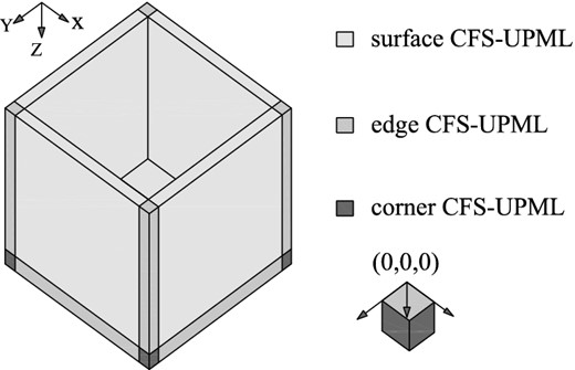
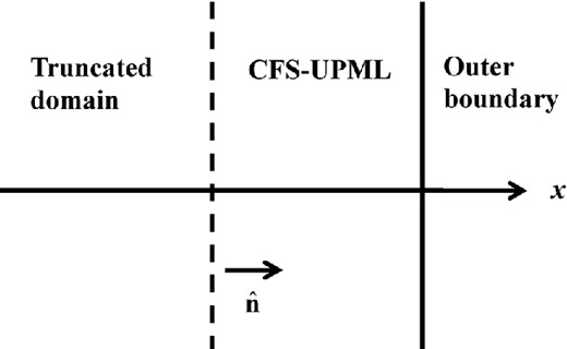
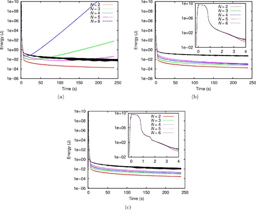
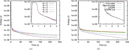
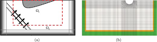
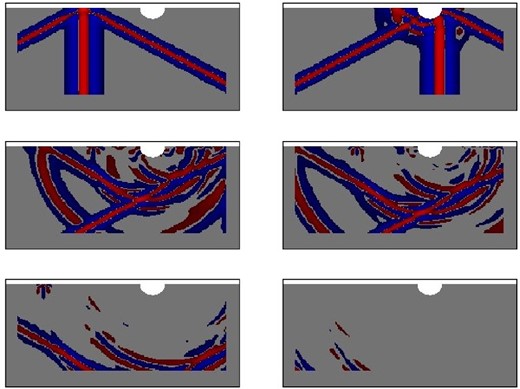
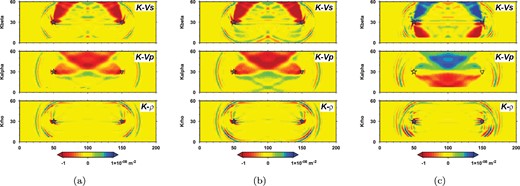
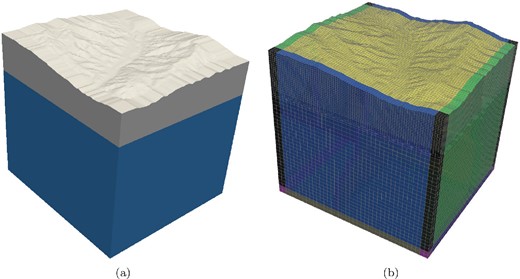
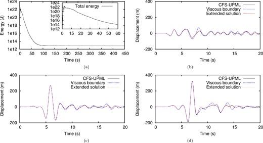
