


Abstract
We demonstrate the feasibility of high-resolution seismic array imaging based on teleseismic recordings using full numerical wave simulations. We develop a hybrid method that interfaces a frequency–wavenumber (FK) calculation, which provides analytical solutions to 1-D layered background models with a spectral-element (SEM) numerical solver to calculate synthetic responses of local media to plane-wave incidence.This hybrid method accurately deals with local heterogeneities and discontinuity undulations, and represents an efficient tool for the forward modelling of teleseismic coda (including converted and scattered) waves. We benchmark the accuracy of the SEM-FK hybrid method against FK solutions for 1-D media. We then compute sensitivity kernels for teleseismic coda waves by interacting the forward teleseismic waves with an adjoint wavefield, produced by injecting coda waves as adjoint sources, based on adjoint techniques. These sensitivity kernels provide the basis for mapping variations in subsurface discontinuities, density and velocity structures through non-linear conjugate-gradient methods. We illustrate various synthetic imaging experiments, including discontinuity characterization, volumetric structural inversion for the crust or subduction zones. These tests show that using pre-conditioners based upon the scaled product of sensitivity kernels for different phases, combining finite-frequency traveltime and waveform inversion, and/or adopting hierarchical inversions from long- to short-period waveforms could reduce the non-linearity of the seismic inverse problem and speed up its convergence. The encouraging results of these synthetic examples suggest that inversion of teleseismic coda phases based on the SEM-FK hybrid method and adjoint techniques is a promising tool for structural imaging beneath dense seismic arrays.
1 INTRODUCTION
Seismic tomography is a fundamental tool in revealing the 3-D structure of the Earth's interior at all scales (e.g. Romanowicz 1991, 2003; Rawlinson et al.2010; Liu & Gu 2012). The resultant 3-D images provide crucial evidence for the tectonic evolution and internal geodynamic processes of our planet (e.g. Dziewonski 1984; Masters et al.2000; Li et al.2008; Fukao et al.2009; Zhao et al.2013). Driven by the continued demand for higher resolution images, and thanks to the proliferation and technological development of seismic instruments, seismic tomography has experienced rapid advances over the past three decades (e.g. Romanowicz 2008; Rawlinson et al.2010). However, owing to the very uneven distribution of seismicity, regional tomography used to rely mainly on transmitted primary phases of global earthquakes (such as P; e.g. Aki et al.1977), and often resolved a refined regional model embedded in a coarser global model (e.g. Spakman & Nolet 1988; Fukao et al.1992; Li et al.2008). In recent years, with the growing deployment of broad-band arrays and the rapid increase in data availability, traditional body-wave tomographic techniques have been adapted by measuring multichannel cross-correlation traveltimes of teleseismic waves at array stations (e.g. Vandecar & Crosson 1990), and attributing traveltime anomalies to structures beneath arrays (e.g. Sandoval et al.2004; Jiang et al.2009; Hung et al.2011). Similarly, surface waves phase velocity maps for array regions are often inverted by regarding the incident fields as two- or multiplane waves (e.g. Friederich & Wielandt 1995; Forsyth et al.1998; Yang & Forsyth 2006). Overall, array analysis has brought great vitality to the quest for regional structures around the globe (e.g. Nolet et al.2005; Gu 2010; Chang & van der Lee 2011; Obrebski et al.2011). On the other hand, coda waves such as converted, reflected and scattered waves that are singly or multiply scattered by heterogeneities distributed beneath the surface, are prevalently used in the imaging of crust and upper-mantle structures beneath seismic arrays. As primary phases are affected mainly by long-wavelength structures (e.g. Wu & Toksoz 1987; Liu & Gu 2012), scattered phases are sensitive to short-wavelength structures, the use of scattered waves in seismic tomography, in principle, will offer substantially higher imaging resolution beneath seismic arrays (e.g. Bostock et al.2001; Frederiksen & Revenaugh 2004; Rondenay 2009). Indeed, converted seismic waves have been used extensively to identify and characterize discontinuities of material properties in the subsurface for more than three decades since the advent of the powerful receiver function (RF) technique [e.g. Langston (1977); Vinnik (1977); Zhu & Kanamori (2000); Kind et al. (2012), see Rondenay (2009) for a review]. Different from point estimates of Moho depth through single station stacking (e.g. Zhu & Kanamori 2000; Yan & Clayton 2007), migration methods, prevalent in active-source exploration, map subsurface discontinuities and scatterers more generally through common conversion point (CCP) stacking, and produce 2- and 3-D stacked images of relative scattering potential beneath linear arrays (e.g. Revenaugh 1995; Sheehan et al.2000). Bostock et al. (2001) introduced an inversion technique based on the Generalized Radon Transform to recover perturbations of elastic properties of the lithosphere beneath dense, passive seismic arrays from teleseismic coda waves. However, the principles of converted-/scattered-wave analysis are still rooted in the ray-theoretical treatment of the seismic waves equation (Rondenay 2009). These ray-based techniques may be appropriate for smoothly varying media, but are less accurate for imaging geologically and tectonically complex structures (e.g. Tape et al.2009, 2010).
Shang et al. (2012) proposed a teleseismic reverse-time migration method to map interfaces in the crust and mantle beneath very dense seismic arrays. By making no assumptions on the presence or properties of interfaces, this wave-equation-based migration method numerically backpropagates transmitted waves from receivers and cross-correlates the P and S constituents to obtain an inverse scattering transform. Numerical solvers that capture complex wave phenomena and allow the use of smooth 3-D background models help produce more coherently migrated images compared to the RF techniques (such as CCP). However, the requirement that station spacing be less than half of the minimum horizontal apparent wavelength to avoid aliasing effect limits its applicability to the majority of current seismic array deployments.
Parallel to the development of array analysis for subsurface imaging, seismic tomography is also transiting from ray-based inversions using 1-D reference models towards adjoint tomography based on 3-D reference models (e.g. Tromp et al.2005; Chen et al.2007; Tromp et al.2008; Fichtner et al.2009; Tape et al.2009), see Liu & Gu (2012) for a review. The latter approach takes advantages of full 3-D numerical simulations in forward modelling and sensitivity kernel calculation, and iteratively refines velocity models through non-linear optimization techniques. Adjoint tomography naturally and automatically includes as many fitted segments of seismograms as 3-D reference models allow over iterations, thus making identification of primary phases unnecessary (e.g. Maggi et al.2009; Tape et al.2010; Lee & Chen 2013). It significantly improves the seismic imaging of 3-D heterogeneous structures with strong velocity contrasts and has become the state-of-the-art technique for high-resolution imaging of various tectonically complex regions in the past few years (e.g. Chen et al.2007; Fichtner et al.2009; Tape et al.2009; Zhu et al.2012). Another notable feature of adjoint tomography is that the topography of interfaces can be determined in junction with volumetric material properties (Liu & Tromp 2008), prompting its use in mapping crustal and mantle discontinuities.
However, for regions with limited seismicity, seismic imaging relies mainly on teleseismic records. As numerical simulations of seismic waves below the period of 8 s at the scale of the globe are still computationally prohibitive, given standard cluster access (e.g. Komatitsch et al.2005; Tromp et al.2008), application of adjoint tomography to teleseismic waves at the frequencies relevant to regional high-resolution imaging (e.g. 1–2 s for P waves and 3–6 s for S waves as in RF and scattering imaging studies) is far from practical (Liu & Gu 2012; Monteiller et al.2013). However, an adapted version of adjoint tomography, where the forward calculation is given by the interfacing of localized 2-/3-D numerical simulation with a fast computed 1-D solution on the boundary, will inherit all the advantages of adjoint tomography while drastically reducing the amount of computation involved. Of course, the assumption behind this hybrid approach is that for coda waves of teleseismic phases, only 2-/3-D effects inside the detailed computational domain matter, while 2-/3-D effects outside the domain are negligible, and only 1-D incident wavefield is computed. Indeed, interfacing of solutions to either 1-D layered model (Roecker et al.2010; Liu & Chen 2011; Pageot et al.2013) or 1-D spherical earth model (Chevrot et al.2011; Monteiller et al.2013) with spectral-element (SEM) solvers has been proposed to speed up forward simulations. Similar hybrid approaches have been used in previous studies of topography and basin effects for ground motion predictions (Bielak & Christiano 1984; Moczo et al.1997; Bielak et al.2003; Krishnan et al.2006; Semblat et al.2008). For example, two-step domain-reduction methods, which first calculate the ground motion for a background structure with localized geological features removed, and then simulate responses of a reduced region with the localized features, have been used to model earthquake ground motion in heterogeneous regions with large localized contrasts in wave speeds (Bielak & Christiano 1984; Bielak et al.2003). To efficiently calculate seismic wavefields for localized 2-D near-surface structures embedded in a 1-D horizontally layered background medium, Zahradnik & Moczo (1996) combined the discrete-wavenumber (DW) solution of 1-D background model with the finite-difference (FD) simulations of local 2-D structures. Wen & Helmberger (1998) developed a P–SV hybrid method, which interfaces the generalized ray theory (GRT) solutions with FD calculations to model seismic wave propagation in the ultra-low velocity zone near the core–mantle boundary. Chen et al. (2005) used a similar hybrid method to study the lithospheric and upper-mantle structures. Zhao et al. (2008) further developed the GRT-FD hybrid method to calculate synthetic seismograms for 2-D localized heterogeneous and anisotropic media. To implement full waveform teleseismic tomography, Roecker et al. (2010) interfaced a 2-D spectral domain FD method with plane-wave propagation through a 2.5-D elastic medium. Although computationally efficient, the use of FD scheme defined on a regular grid still presents limitations on handling complex 2-D geological models with large free-surface or interface topography, as often encountered in practice (Zhou et al.2012; Zheng et al.2013). To overcome this limitation, a more geometrically flexible method, such as the finite-element method (FEM) or SEM may be used to conduct forward modelling. Following the work of Chevrot et al. (2004), Godinho et al. (2009) and Chevrot et al. (2011), Monteiller et al. (2013) proposed a hybrid method that interfaces a direct solution method (DSM) for 1-D spherical earth with a SEM to compute short-period synthetics for teleseismic body waves in 3-D regional models.
As the wave fronts of teleseismic waves entering the upper mantle (above 410 km) beneath most seismic arrays can be safely assumed to be planar (Rondenay 2009), analytical methods such as frequency–wavenumber (FK) method can be used to precisely and efficiently compute plane-wave responses of 1-D medium (Zhu & Rivera 2002). A full numerical simulation can be then initiated to calculate the synthetic response of local 2-D/3-D media to plane-wave incidence, while at the boundaries, field values are exchanged with 1-D FK solutions, and scattered waves are absorbed by absorbing boundary conditions (Liu & Gu 2012). This hybrid method may efficiently model the high-frequency coda of main teleseismic phases, which consist largely of energy scattered off small heterogeneities in the receiver-side media. It combines the efficiency of analytical methods for 1-D background media with the accuracy of full numerical simulations for 2-D/3-D media, and accurately captures the interactions between teleseismic waves and heterogeneous structures beneath seismic arrays.
In this paper, we thus develop an SEM-FK hybrid method to calculate the synthetic response of local media to teleseismic plane-wave incidence for the modelling of teleseismic coda waves. The SEM accurately handles large velocity contrasts and undulating surfaces and discontinuities through a precisely designed finite-element mesh, and achieves exponential convergence properties of spectral methods (Komatitsch & Tromp 1999; Cohen 2002; De Basabe & Sen 2007; Seriani & Oliveira 2008). It has shown to be an efficient solver for effective modelling of complex media (Komatitsch et al.2004; Stupazzini 2006; Lee et al.2008; Peter et al.2011). As numerical calculations are limited only to localized regions of interest, the SEM-FK hybrid method that we introduce can simulate the local propagation of teleseismic waves at very high frequencies. Hereafter, we first present the theory of the SEM-FK hybrid method, and then benchmark it against FK solutions for a 1-D layered model in Section 2. In Section 3, we give a brief introduction to adjoint tomography, which utilizes the forward SEM-FK calculations. We conduct synthetic tomographic tests for various models in Section 4 to demonstrate the promising resolving capabilities of adjoint tomography with teleseismic coda waves, for both subsurface interfaces and velocity anomalies.
2 SEM-FK HYBRID METHOD
2.1 FK method
In this study, we are interested in modelling responses of local heterogeneities to teleseismic body-wave incidence. For computational efficiency, we assume the wave fronts of teleseismic body waves to be planar when they arrive in the upper mantle beneath a seismic array with a limited aperture (Rondenay 2009), which can then be propagated into a local medium. As shown in Fig. 1, the plane waves impinge from the half-space below a stack of n layers with an incidence angle θ, and soon enter a target region (grey shaded box) which assumed to contain all local heterogeneties (Roecker et al.2010). The interactions of plane waves with these heterogenities will generate scattered waves, which can be recorded as coda (sometimes precursor) waves by seismic stations at the free surface.
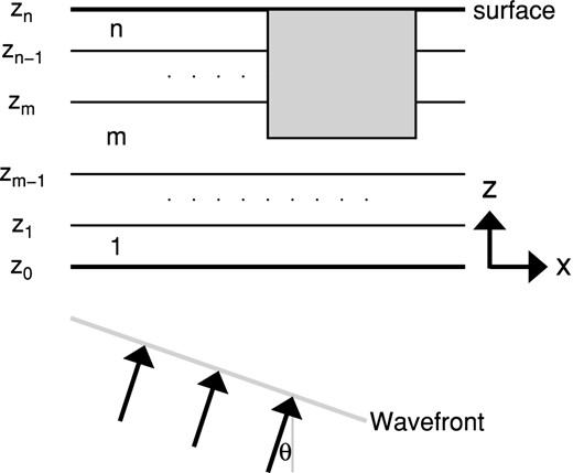
An n-layer over half-space model. The grey shaded region is the computational domain in which the spectral element method is applied. Teleseismic plane waves with an incidence angle θ enter from the bottom of the stacked layers. For simplicity, the interface between the bottom layer and the half-space is assumed to be located at z0 = 0.
We adapt the propagator matrix method (e.g. Haskell 1953; Takeuchi & Saito 1972) to compute the displacement response of a stack of layers to incident P and S plane waves from the half-space below. It uses the Thompson–Haskell propagator matrix technique to obtain the displacement field at any point within the n-layer over a half-space (Thomson 1950; Haskell 1962; Zhu et al.2012). When free surface boundary condition and unit amplitude of incident waves are applied, the wavefields can be uniquely determined. We formulate the FK algorithm for plane-wave incidences and present its tenets in the Appendix.
2.2 SEM
For 2- and 3-D heterogeneous media, the analytical techniques (such as the FK method discussed in the Appendix) can no longer adequately capture the complex wave propagation phenomena related to interactions with local heterogeneities, and numerical solvers have to be used. The SEM is a class of numerical methods that is currently widely used to simulate seismic wave propagation in heterogeneous media at both regional (e.g. Komatitsch et al.2004; Peter et al.2011) and global (e.g. Komatitsch & Tromp 2002a,b; Tromp et al.2008) scales [see Chaljub et al. (2007) for a review]. It combines the flexibility of the finite-element method with the accuracy of spectral techniques and has good accuracy and convergence properties (Peter et al.2011). With its flexible mesh design, the SEM readily incorporates surface topography and internal material interfaces, and with its high numerical accuracy it can tackle complex wave propagation in full detail.
To conduct feasibility studies of an SEM-FK hybrid method and its application to seismic imaging, we use the open-source software package SPECFEM2D, downloaded from Computational Infrastructure for Geodynamics (CIG) website (http://www.geodynamics.org). It is designed to simulate both forward and adjoint seismic wave propagation in 2-D acoustic, (an)elastic, poroelastic or coupled-(an)elastic-poroelastic media, although in this paper we focus mainly on the elastic properties of the media (i.e. density and P- and S-wave velocities). This package has the flexibility of handling both structured or unstructured meshes. For subhorizontally layered earth models, an internal mesher in the package can be used to generate quadrilateral mesh for later spectral-element simulations. For more complex 2-D models, external mesh generation tools need to be employed to honour all discontinuities and interfaces present in the models (e.g. Blacker et al.1994; Casarotti et al.2008; Peter et al.2011), such as the CUBIT software package (http://cubit.sandia.gov/). The SPECFEM2D package also includes the capability of computing finite-frequency kernels for seismic inversion purposes (see Section 3.1). In this paper, we use CUBIT mesher for forward wave simulations in Section 2.3.2 and synthetic data calculations in Section 4.3. And for all other models as well as simulations in adjoint inversions, we apply the internal mesher.
2.3 SEM-FK hybrid method
When plane waves travelling upwards from the half-space through a stack of layers encounter local heterogeneities, which are encompassed by a domain drawn as a grey box in Fig. 1, reflected or scattered waves are generated within the domain through interactions between the incoming seismic waves and heterogeneous local structures. With displacement and traction of the 1-D background medium supplied by the FK method for the boundary, we can apply the SEM in the grey box to simulate the continued plane-wave propagation into the heterogeneous domain.
2.3.1 Benchmark for 1-D models
Because of the flexibility of the SEM in dealing with subsurface discontinuities and heterogeneities, the SEM-FK hybrid method can be used to investigate the effect of local heterogeneous media on the coda waves of teleseismic main phases. Before proceeding further, let us first demonstrate the accuracy of SEM-FK by benchmarking it against FK solutions for purely 1-D media, that is, having no local lateral anomaly.
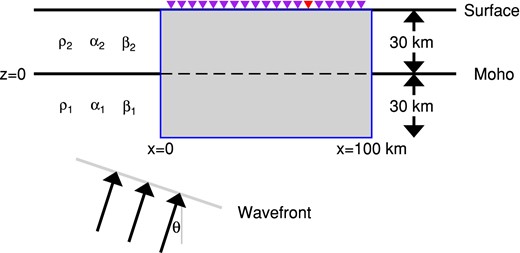
One layer over half-space model for SEM-FK benchmarking. The top and bottom layers have the typical velocities of the crust and mantle given in Table 1. The thickness of the crust is 30 km. The grey shaded region with a size of 100 × 60 km is the computational domain for the SEM, which may include undulated Moho (black dashed line) and heterogeneous density, Vp and Vs structures. Dense seismic arrays (inverse triangles) are placed along the free surface of the domain. The left boundary of this domain and the Moho discontinuity together define the local Cartesian coordinate system. This model also serves as the background model for various synthetic tests in Section 4.
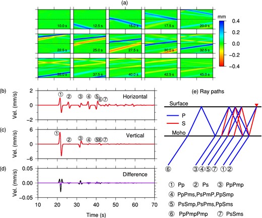
(a) Snapshots of horizontal-component displacement field computed by the SEM-FK hybrid method in a one-layer-over-half-space model (Fig. 2 and Table 1) due to a P plane wave with 15° incidence angle. (b) Horizontal- and (c) vertical-component velocity seismograms generated by the FK (blue) and SEM-FK hybrid (red) methods for a receiver located at x = 70 km on the surface (red triangle in Fig. 2) with various coda phases identified. (d) Differences between the FK and SEM-FK seismograms for the horizontal (purple) and vertical (black) components. Note that different vertical scales are used from (b) and (c). In (e) we have drawn the ray paths of various coda phases, with blue and red line segments showing the P and S legs, respectively.
Material properties for the one-layer-over-half-space (e.g. crust-over-mantle) model in Fig. 2.
| Density ρ (kg m−3) | Vp (m s−1) | Vs (m s−1) | |
|---|---|---|---|
| Crust | 2600 | 5800 | 3198 |
| Mantle | 3380 | 8080 | 4485 |
| Density ρ (kg m−3) | Vp (m s−1) | Vs (m s−1) | |
|---|---|---|---|
| Crust | 2600 | 5800 | 3198 |
| Mantle | 3380 | 8080 | 4485 |
2.3.2 Plane-wave incidence to a 2-D medium
To demonstrate the capability of the SEM-FK hybrid method in dealing with local heterogeneities, we show an example of the interaction of incoming P plane waves with a subducted slab. The computational domain, of size 200 km × 200 km, consists of the crust and uppermost mantle, with material properties given in Table 1. A subducted slab with a +4.0 per cent density and velocity perturbation is present in the mantle (Fig. 4j). As the FK method is only valid for layered models, we taper material properties at the left and right edges of the subducted slab. A P plane wave with a 15° incidence angle impinges on the bottom left corner of the computational domain at time t = 5 s. A cut-off frequency of f0 = 1 Hz and maximum amplitude of 1 mm is used for this example. The mesh for this example is built with the CUBIT software package (Section 2.2) to accurately account for the geometry of the subducted slab. Figs 4(a)–(i) show snapshots of the horizontal displacement field computed by the SEM-FK hybrid method. The incident waves are reflected by or transmitted through the lower and upper slab boundaries (Figs 4c and d) as well as the Moho (Fig. 4e) and then reflected by the free surface (Fig. 4f). To further demonstrate the effect of the slab on seismic wave propagation, horizontal-component displacement recorded by 20 receivers at the surface is shown in Fig. 5. The arrivals of the main phase and coda phases labelled in Fig. 3(e) can be clearly identified in Fig. 5 (dashed lines). These coda waves will be critical in the detailed mapping of slab structures in the synthetic tests discussed in later sections.
Snapshots of horizontal displacement (a–i) computed by our SEM-FK hybrid method in a heterogeneous model with a subducted slab (j). The computational domain, of size 200 × 200 km, consists of the crust and the uppermost mantle (Table 1), as well as a subducted slab with a +4.0 per cent density and velocity perturbation in the mantle.
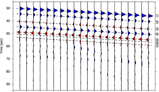
Horizontal-component displacement seismograms generated by the SEM-FK hybrid method for a subducted slab model ( Fig. 4j). They are recorded by 20 evenly spaced receivers at the top surface of the computational domain. The seven dashed lines denote the predicted arrival times of the seven Moho related phases labelled in Fig. 3(e).
3 BRIEF SUMMARY OF THE THEORY OF ADJOINT TOMOGRAPHY
Over the past three decades, discontinuity characterization using converted seismic waves and the determination of volumetric material properties by seismic tomography have formed the set of core methodologies used in seismic imaging of the solid Earth at regional and global scales. These two families of methods provide complementary means of mapping the internal structures of the Earth (Rondenay 2009). Actually, observed seismograms depend on variations in both material discontinuities and volumetric material properties. In the framework of adjoint tomography, we can determine simultaneously the internal discontinuity undulations and the variations of volumetric material properties (e.g. density, wave speeds). Here we only summarize the theoretical aspects of adjoint tomography in 2-D for later sections. More details can be found for instance in Tarantola (1984), Tromp et al. (2005), Liu & Tromp (2006), Tape et al. (2007), Liu & Tromp (2008), Tromp et al. (2008), Fichtner et al. (2009), Tape et al. (2009) and Liu & Gu (2012).
3.1 Fréchet kernels
3.2 Non-linear CG method
As only the gradient g(m) is needed for model update, the non-linear CG method is characterized by low memory and computation requirements compared to Newton's methods. It has good local and global convergence properties (Hager & Zhang 2006), and provides successively improving approximations to the true solution, which may reach the tolerance threshold after relatively fewer number of iterations compared with the steepest descent method and linear CG method (Saad 2003). Nonetheless, properly designed pre-conditioners could help improve the convergence rate of the non-linear CG method (Hu et al.2011).
4 SEISMIC ARRAY IMAGING
The SEM-FK hybrid method developed in Section 2 provides a tool to accurately calculate responses of local heterogeneities to incident plane waves. Based upon the Fréchet kernels computed by an adjoint method, we can exploit the sensitivities of various phases to both subsurface discontinuities and volumetric material properties. Furthermore, we can iteratively update the model by a non-linear CG method and achieve optimized models that are consistent with seismic data. In this section, we show the results of several synthetic tests and demonstrate the feasibility of high-resolution seismic array imaging based upon teleseismic converted/coda waves.
4.1 Discontinuity mapping
In the first example, a target model is built by making the Moho of a layer-over-half-space model (given in Table 1 and Fig. 2) vary with an undulated sinusoidal shape having a maximum variation of 3 km (black curves in Fig. 6). We then compute seismic wave propagation for eight teleseismic events with P plane-wave incidence angles of 4°, 12°, 20° and 28° (from both left and right) based upon our SEM-FK hybrid method. The incidence angles are restricted to the range of [−30°, 30°] to reflect those of most teleseismic arrivals, where negative (or positive) angles represent plane-wave incidence from the lower left (or right) side of the model. All plane waves have a Gaussian source-time function with a cut-off frequency of 2 Hz, and 10 receivers with equal spacing of 10 km are deployed along the surface to record synthetic data.
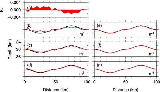
(a) Moho discontinuity kernel Kd (in the unit of 10−6 m s−1) based on the starting two-layer model for the Ps converted waves with a source cut-off frequency of 2 Hz. (b)–(g) Updated models of Moho variations (red curves) over six iterations. The true Moho variation (black curves) follows a sinusoidal function with a maximum amplitude of 3.0 km. The vertical-to-horizontal exaggeration ratio is 2:1. Inversions are based on synthetic data recorded by 10 surface stations with an equal spacing of 10.0 km.
In this case, we restrict inversions to Moho depth only and ignore other volumetric model parameters. As the arrivals of Moho-converted Ps waves are strongly affected by the Moho depth, we first invert the Ps waveforms in the synthetic data to recover Moho undulations. The starting model is chosen to be the 1-D background model with a flat Moho at 30 km depth (Fig. 2). Since converted Ps waves are most prominent on the horizontal components (Fig. 3), only horizontal components of Ps waveforms are identified and inverted.
For illustration purposes, the discontinuity kernel Kd computed based on eq. (9) for the Ps waves in the starting model is shown in Fig. 6(a). Even though the starting model has only a flat Moho, the depth kernel is informative on the necessary Moho variations to approach the ‘target’ Moho. The sign of the kernel is opposite to that of Moho topography update, while the amplitude of the kernel provides information on the magnitude of Moho variation needed in the first iteration. This and the consecutive versions of Moho kernel are smoothed using a radius of σ = 1.5 km in eq. (13).
Based upon the depth sensitivity kernels computed by the adjoint technique and the non-linear CG optimization method discussed in Section 3.2, we iteratively improve the Moho variations (Figs 6b–g). We remesh the model with the internal mesher at each iteration after the Moho depth has been updated. The Moho is fully recovered after six iterations, as demonstrated by the comparison between synthetic data (black traces) and synthetics (red traces) for the initial model, and models obtained at the third and sixth iterations (Figs 7a–c). Synthetics calculated for the sixth model match the synthetic data almost exactly (Fig. 7f). The misfit ϕ value is also reduced to less than 0.1 per cent of the initial misfit (Fig. 7g) after these six iterations.
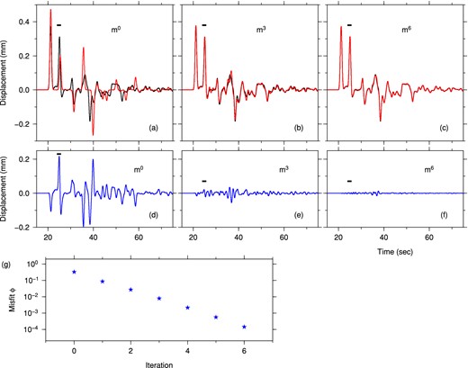
(a)–(c) Comparison of horizontal-component synthetic seismograms (red traces) recorded by the station located at x = 65 km for the initial model, and models obtained at the third and sixth non-linear CG iterations, with synthetic data (black traces). The time range of the Ps waves used in the inversion is indicated by black horizontal bars, and a Welch window function is applied over this time interval. (d)–(f) Differences between synthetic data and synthetic seismograms shown in (a)–(c). (g) Iterative reduction of the misfit function value. The unit of the misfit function ϕ is 10−6 s m2.
This numerical example clearly demonstrates the feasibility of Moho discontinuity inversions based on converted Ps waveforms. Note that receiver spacing (10 km) is about six times the wavelength of the shear waves (∼1.6 km). Posing the imaging problem as an iterative inverse problem avoids the formal anti-aliasing requirement (i.e. receiver spacing having to be less than half of the wavelength) in some other imaging techniques (Shang et al.2012). Also note that images obtained from migrating Ps waveforms, known to be related to the inverted Moho from the first adjoint iteration (Fig. 6b) may still be quite far from the true Moho variations (Tarantola 1984). However, station spacing that is too wide may introduce artefacts in the inverted images, as shown by a similar numerical test with 22.5 km station spacing in Fig. 8. As expected, the inverted Moho has large unwanted oscillations and contains high frequency noise after six iterations. In practice, if other Moho-related phases (such as PmPmp and PmPms) can be clearly identified (Fig. 3) in seismic recordings with high signal-to-noise ratio, Ps and these later phases can be inverted simultaneously to speed up the recovery of Moho geometry as they have complementary sensitivities to the Moho depth variations.
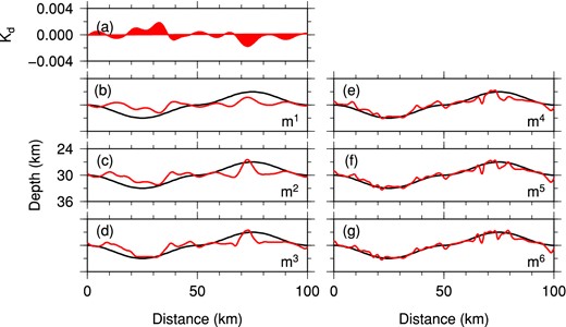
Similar to Fig. 6, but only horizontal Ps waveforms from five surface stations with a spacing of 22.5 km are used in the inversion.
4.2 Volumetric structural inversion
4.2.1 Ps waveform inversion
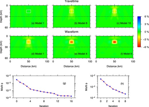
In the second example, we first demonstrate the inversion of converted Ps waves for volumetric structures only. We design a target model that contains a 6.0 per cent slower mid-crustal Vs anomaly (12 km × 8 km white box in Fig. 9) in the two-layer background model (Table 1). This slow anomaly is expected to affect the arrival time of the Ps phase and produce scattered waves at nearby stations above the anomaly. No Vp or density perturbation is introduced such that P arrival times remain the same for all stations. The same eight events are used and the receiver spacing at the surface remains 10.0 km as in Section 4.1, but the cut-off frequency of incident plane waves is reduced to 1 Hz.
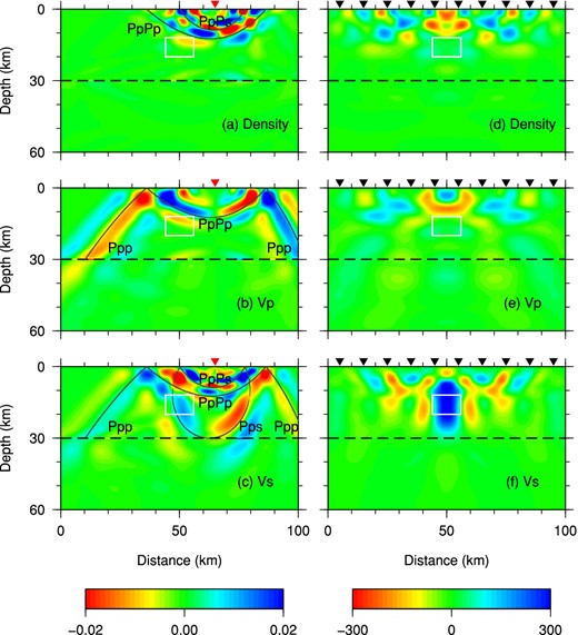
Density (a,d), Vp (b,e) and Vs (c,f) kernels of Ps converted waves computed for the starting model of Fig. 2. All these kernels have the unit of 10−14 s. (a)–(c) are the sensitivity kernels corresponding to a single event and station pair. The event has an incidence angle of 12° from the left and the station is located at x = 65.0 km on the surface. The grey curves denote the isochrons of forward-scattered Ppp, Pps and backscattered PpPp, PpPs over the time window of the Ps arrival. (d)–(f) are the smoothed gradients of the misfit function ϕ for all events and receivers. Colour bars reflecting the amplitude of the kernels for (a)–(c) and (d)–(f) are shown at the bottom.
Assuming no prior knowledge of the location and magnitude of structural anomalies in the model, we simultaneously update density and velocity structures. Let us first show the unsmoothed density (Fig. 9a) , Vp (Fig. 9b) and Vs (Fig. 9c) kernels calculated for the Ps waveform misfit in the initial model of a particular event (with a 12° incidence angle) recorded by a station located at x = 65.0 km (i.e. sensitivity kernels for one source–receiver pair). These individual kernels clearly delineate various isochrons for waves scattered off possible density, Vp and Vs heterogeneities arriving in the selected Ps time window (e.g. Bostock et al.2001). The density kernel (Fig. 9a) is sensitive to backscattered waves such as PpPp (i.e. Moho-transmitted and surface-reflected PpP waves scattered into P waves) and PpPs (PpP scattered to S) waves. The Vp kernel (Fig. 9b) is mainly sensitive to P-to-P scattered waves (Wu & Aki 1985; Rondenay et al.2008), such as Ppp (Moho-transmitted Pp waves scattered to P waves) and PpPp waves. As Vs anomalies result in both P-to-P and P-to-S scattering, the Vs kernel in Fig. 9(c) is sensitive to all the scattered waves, including Ppp, PpPp, PpPs as well as Pps (Pp scattered to S). Note that the Pps isochron is tangent to the Moho discontinuity at the position where the incoming P waves are transmitted and converted to S waves.
Even though individual kernels may not resemble the embedded anomaly, the misfit kernels (i.e. Fréchet kernels of the total misfit ϕ), computed by summing up individual kernels for all events and stations, should provide clues to possible locations of velocity anomalies. The smoothed kernels of total Ps waveform misfits for the initial model are shown in Figs 9(d)–(f). Indeed, the shear velocity misfit kernel (Fig. 9f) correctly identifies the slow anomaly in the white box, and provides model update for the next iteration. The misfit kernels for P-wave velocity (Fig. 9e) and density (Fig. 9d) also suggest probable changes in Vp or density distributions, although in this case, much weaker and mostly outside the white box. This is not surprising considering that the selected windows for the transmitted Ps phase may also include other scattered arrivals as indicated by the isochrons in Figs 9(a)–(c).
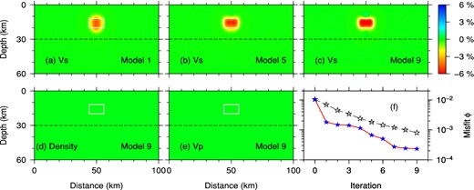
Although no density or Vp anomalies exist in the target model, we still simultaneously invert for density, Vp and Vs structures based on the non-linear CG algorithm, and we examine the ability of the inversion process to attribute the misfit to the correct parameters (in this case Vs). The successively updated Vs models are shown in Figs 10(a)–(c). After nine iterations, no significant improvement in model or reduction in misfit ϕ is observed and the inversion is terminated (Fig. 10f). The final recovered slow Vs anomaly (Fig. 10c) coincides very well with the white box. On the other hand, no obvious structural anomalies can be identified in the final recovered density and P-wave models after nine iterations (Figs 10d and e), although some very weak artefacts may be visible near the surface. However, the recovered Vs anomaly has an average variation of 1.8 per cent, smaller than the presumed 6 per cent. This may be partly explained by the fact that out of the total 80 horizontal Ps waveforms used, only a few are sensitive to the small crustal anomaly and thus have limited recovery ability in the iterative process. To increase the recovered amplitude of the Vs anomaly and reduce the effect of artefacts, it may be beneficial to use more events, more stations, and include both the main P phase and/or longer coda phases (e.g. PpPs, PsPs) in the waveform inversion. Nonetheless, this numerical example verifies the capability of the SEM-FK method and adjoint tomography to map volumetric subsurface structures based on teleseismic converted/scattered waves.

(a)–(c) Updated Vs structures for the first, fifth and ninth iterations of an inversion of Ps waveform only. A 6.0 per cent slower Vs anomaly is placed in the mid-crust as the target model. No variation in density or P velocity is assumed. The background is the two-layer model of Fig. 2 and Table 1, and the Moho is indicated by the dashed black line. (d) Density and (e) Vp perturbation structures after the ninth iteration. No obvious density or Vp anomaly can be identified. (f) Iterative reduction of the misfit function value. The unit of the misfit function ϕ is 10−6 s m2.
4.2.2 Ps waveform inversion with pre-conditioner
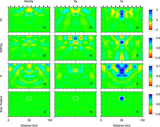
Smoothed kernels of the misfit function ϕ with respect to density (a,d,g), Vp (b,e,h) and Vs (c,f,i) computed for the starting model (Fig. 2) for different phases. All the kernels in (a)–(i) have the unit of 10−12 s. (a)–(c) Kernels of Ps converted waves, (d)–(f) kernels of PpPmp waves and (g)–(i) kernels of all the remaining coda waves following the PpPmp phase (shortened as X). (j) Scaled product of density kernels in (a,d,g). (k) Scaled product of Vp kernels in (b,e,h). (l) Scaled product of Vs kernels in (c,f,i). The target model contains a 6.0 per cent slower Vs perturbation in the white box.
We perform a Ps waveform inversion with the above pre-conditioner and show the results of the first nine iterations in Fig. 12. The final model shows that the slow Vs variation within the white box is well recovered by inverting only the Ps waveforms, and thanks to the pre-conditioner, the amplitude of the slow Vs anomaly (−6 per cent) is much better recovered (with an average variation of 5.02 per cent) than in the example above without the pre-conditioner (Section 4.2.1 and Fig. 10). The scaled products of kernels for different seismic coda phases clearly provide very good guidance on the update of structural anomalies. In addition, the use of this pre-conditioner also significantly speeds up the convergence of the Ps waveform inversion as indicated by the faster reduction of misfit values shown in Fig. 12(f).
(a)–(e) Same as Fig. 10, but a pre-conditioner from the scaled products of kernels for different coda waves is used in the waveform inversion. (f) Iterative reduction of the misfit function values for inversions with a pre-conditioner (denoted by blue stars) and without a pre-conditioner (denoted by empty stars, also shown in Fig. 10f).
4.2.3 Combined traveltime and waveform inversion
Previous studies have shown that wave-equation based traveltime tomography can resolve velocity anomalies similar to the size of the first Fresnel zone, while reflected/scattered waveform inversion resolves structures of a size close to the dominant wavelength (e.g. Wu & Toksoz 1987; Virieux & Operto 2009; Liu & Gu 2012). This suggests that a combined traveltime and waveform inversion may be an efficient tool to recover subsurface structures at successively decreasing scales. As a synthetic example, we assume a target model with a 6.0 per cent slower Vp anomaly in the mid-crust, at the same location as the Vs anomaly in Sections 4.2.1 and 4.2.2. Note that Vp anomalies are more difficult to resolve from coda phases than Vs anomalies because they can only be imaged by P-to-P scatters (Wu & Aki 1985; Rondenay et al.2008; Pageot et al.2013). On the other hand, the arrival times of the direct P phase at some stations will be delayed by the slow Vp anomaly, thus complementing the coda waves in sensitivity. We start from a two-layer model and invert the traveltime misfits of the direct P phase to obtain a 2-D starting tomography model for later waveform inversion. The use of an improved 2-D starting model will reduce discrepancies of coda waves between data and synthetics, hence speeding up the convergence of the non-linear CG method.
The same set of event incidence angles and stations as in Section 4.2.1 is used in these inversions with the cut-off frequency of 1 Hz. Fig. 13 shows density, Vp and Vs kernels of the direct P-wave cross-correlation traveltime misfit for individual source–station pair (Figs 13a–c), as well as all sources and stations combined (Figs 13d–f). Clearly, individual density kernel (Figs 13a) is sensitive to impedance contrast across the Moho and near the surface, while individual Vp (Fig. 13b) and Vs (Fig. 13c) kernels mainly cover the first Fresnel zones. Note that these kernels are computed similarly to those in Figs 9(a)–(c), although adjoint sources related to traveltime misfits of the direct P phase are used. The Vp kernel for traveltime misfit of all sources and receivers (Fig. 13e) exhibits positive values in the vicinity of the white box, which suggests a corresponding reduction in Vp. Figs 14(a)–(c) are the iteratively updated Vp models from inversion of only the direct P traveltime, which hints a slow Vp anomaly in the mid-crust after 16 iterations (Fig. 14c). We choose the Vp model from the 16-th iteration (Fig. 14c) of traveltime inversion as the starting model for the subsequent waveform inversion, while utilizing all coda waves following the direct P phase. After eight iterations, the 6 per cent slower Vp anomaly is almost fully covered (Fig. 14f), the average perturbation of the anomaly in the white box being −5.89 per cent.
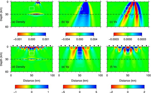
Traveltime sensitivity kernels of density (a), Vp (b) and Vs velocity (c) for the direct P wave of a single event and station pair in the starting model of Fig. 2. The station is placed at x = 65.0 km and the event has an incidence angle of 12°. (d)–(f) Unsmoothed gradients of traveltime misfit function for all events and receivers. All these traveltime kernels have the unit of 10−8 s2 m−2.
Iteratively updated Vp models in a combined traveltime and waveform inversion. For the target model, a −6.0 per cent Vp perturbation with respect to the surrounding background two-layer model is placed in the white box. The dashed black curve denotes the Moho. (a)–(c) Iteratively updated Vp models by inverting traveltime anomalies of the direct P wave. The starting model m0 is the two-layer model of Fig. 2 and Table 1. (d)–(f) Updated models by waveform inversion of coda waves following the direct P phase. The 2-D model in (c) is used as the starting model. (g) and (h) Iterative reduction of the misfit function value of traveltime inversion (g) and coda waveform inversion (h). The units of the misfit functions in (g) and (h) are s2 and 10−6 s m2, respectively.
This synthetic test nicely illustrates the power of combining traveltime inversion of teleseismic main arrivals (e.g. P phase) and waveform inversion of seismic coda waves (e.g. Ps, PpPmp), as the long-period structures determined by traveltime inversion reduce the non-linearity of the waveform misfit and serve as a natural initial model for higher resolution waveform inversions. This is similar to the frequency-domain full waveform inversion methods used in exploration seismology, in which transmission tomography at longer periods generates starting models for subsequent waveform inversions of reflected waves (e.g. Pratt et al.1998; Pratt & Shipp 1999). For regions with seismic array deployments, 3-D traveltime tomography models are routinely inverted based on relative traveltime measurements (e.g. Vandecar & Crosson 1990; Hung et al.2011). Instead of relying on simple smooth 1-D background models, coda-wave imaging may take advantage of these readily available 3-D models and speed up the convergence of waveform inversion.
4.3 Subduction zone models
Subduction zones are crucial components of plate tectonics and mantle geodynamics (e.g. Zhao 2012), and high-resolution images of subduction zones can improve our understanding of the subduction dynamics, arc magmatism and the nucleation of various types of earthquakes. Therefore, to explore the imaging capability of our SEM-FK hybrid technique for subduction zones, let us design two simplified subduction zone models and try to recover them based on teleseismic P and its coda waves.
4.3.1 Fast subducted slab model
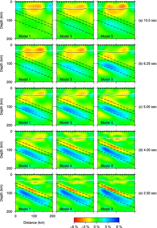
In Section 2, we have investigated the interaction of an incident P plane wave with a simple subduction zone model (Fig. 4j) which included a 51-km-thick and 21.8° dipping subducted slab with 4.0 per cent density, fast Vp and Vs perturbations. In this section, we try to recover this subducted anomaly starting from the two-layer (crust-over-mantle) background model. 10 teleseismic events with incidence angles that evenly sample [−27°, 27°] with an interval of 6° are used to generate synthetic data for the target model. 20 receivers are placed along the surface with an even spacing of 10 km, which is slightly larger than the wavelength of 2.5 s S waves at the surface. To constrain the slab structure, the P wave and all of its coda waves are used in the waveform inversion. In this case, only volumetric model parameters (density, Vp and Vs) are inverted and no Moho variations are included in the inversion. As waveform misfit is highly non-linear, models may be trapped in local minima and never reach the global minimum (i.e. the true model) in the iterative optimization procedure. To avoid local minima and reduce the non-linearity of waveform misfit function, we adopt a hierarchical strategy in which we successively invert waveforms from long period (10 s, f0 = 0.1 Hz) to short period (2.5 s, f0 = 0.4 Hz; Virieux & Operto 2009).
We first start waveform inversions at 10 s, the period at which the wavelength of S waves in the mantle is comparable to the thickness of the slab. The iteratively updated density, Vp and Vs models are shown in Fig. 15(a). The inversion is stopped at the eighth iteration when no more significant reduction in misfit value is observed (Fig. 15c). From model 8 in Figs 15(a), it is clear that most of the slab can be recovered by the 10 s synthetic data. Actually, the contour of the anomalous slab emerges even after one iteration. However, the amplitude of the slab anomaly (4 per cent) are much better until the eighth iteration. This agrees with the discussion in Section 4.2.3 that waveform inversions are capable of resolving anomalous structures of a size similar to the wavelength of the seismic waves used.
Iteratively updated density, Vp and Vs models from waveform inversions of the direct P phase and all of its coda waves. The target model contains a fast slab in a two-layer background model (Fig. 4j). (a) Density, P- and S-wave velocity models obtained by waveform inversions of 10 s synthetic data at the first, fourth and eighth iteration. (b) Similar to (a), but generated by inversion of 2.5 s synthetic data with ‘Model 8’ in (a) as the starting model. (c) Iterative reduction of the misfit function value for waveform inversions of first 10 s and then 2.5 s data. The unit of the misfit function is 10−6 s m2.
However, the sharp top and bottom boundaries of the slab are not very well determined due to the long-period nature of the data. To further refine the inversion results, we restart the waveform inversion with 2.5 s synthetic data, using the final (eighth) model of the 10 s waveform inversion as the starting model. Six iterations are performed in this case (Fig. 15b), and the 4 per cent density and velocity anomaly in the subducted slab is then almost fully recovered. Slab boundaries are more clearly delineated and match well with the target model, especially for Vp model (Fig. 15b). However, artefacts of low-amplitude slow wave speed or negative density anomalies still exist outside the slab in the final models (Model 6 in Fig. 15b). They appear mostly on the lower side of the slab for Vs model, while in both the crust and the mantle wedge for density model. This is not surprising, as the Vp structures are well recovered from the inversion of combined direct P waves and P-to-P scattering in the coda waves, while density structures can only rely on the backscattered waves recorded in the coda. The Vs model is better inverted than density due to its sensitivity to all coda phases (Section 4.2.1). The existence of artefacts below the slabs (Fig. 15b) in the Vs model compared to the Vp model may be a result of the lack of direct S waves in the inversions.
4.3.2 Two-layer subducted slab model
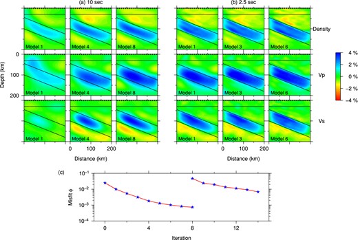
In the last synthetic example, we consider a more realistic and complex subduction zone model inspired by the Alaska subduction zone model imaged by Rondenay et al. (2008) using the Generalized Radon Transform technique. The subducted slab consists of two layers, a slower layer (−6.0 per cent variation in density, Vp and Vs) of subducted oceanic crust atop a fast (4.0 per cent perturbation in all three parameters) subducted lithospheric mantle (Fig. 16b). The anomalies of the slab near the left and right boundaries of the computational domain are tapered to match the 1-D model used in the FK calculation (Fig. 16b). In addition, continental Moho contains a depression of maximal size 10.0 km from its two flat ends. The receiver locations are the same as in the previous example (Section 4.3.1). However, 16 teleseismic events with incidence angles that evenly span [−30°, 30°] at a 4° interval are used to improve image resolution. The teleseismic P wave and all of its coda waves are used to invert for both volumetric anomalies and Moho variations from a two-layer reference model (Fig. 16a). We compute Fréchet kernels for the Moho depth, density, Vp and Vs, and simultaneously invert for both volumetric structural changes and discontinuity variations.
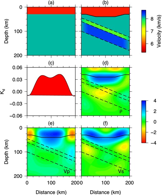
The starting (a) and target (b) Vp model for waveform inversion of a two-layer subducted slab model. Moho discontinuity (c), density (d), Vp (e) and Vs (f) kernels for teleseismic P wave and its coda waves in the starting model. The cut-off period of the incoming P waves is 10 s. The unit of the discontinuity kernel in (c) is 10−6 m·s, and the unit of the volumetric kernels in (d)–(f) is 10−14 s.
Again, a hierarchical inversion strategy is employed from long to short period progressively through 10, 6.25, 5, 4 and 2.5 s waveform data. Inversions proceed to a shorter period when no significant improvement in misfit value is observed in inversion of longer period data, while the final model of the longer period inversion is used as the initial model (i.e. Model 0) for the ensuing shorter-period inversion.
The Moho depth (Fig. 16c), density (Fig. 16d), Vp (Fig. 16e) and Vs (Fig. 16f) misfit kernels for the 10 s waveform data of direct P and coda waves in the starting model (Fig. 16a) clearly highlight the necessary model update in the first iteration. The positive Moho misfit kernel (Fig. 16c) implies a deepening of the central segment of the Moho. The observed large positive values of the density, Vp and Vs kernels in the vicinity of the Moho suggest that a local decrease in the density, Vp and Vs may also reduce waveform misfit, which is another indication of a deeper central segment of the Moho. Kernel amplitudes in the vicinity of the subducted slab are much weaker than those around the Moho, mainly due to the fact that density/velocity perturbations in the subducted slab is either −6.0 per cent or 4.0 per cent, much smaller than the material property contrast between the crust and the mantle. It can thus be predicted that the first model update will be predominantly corrections to the Moho topography, and density/velocity adjustments in the slab will follow in later iterations. Nevertheless, some patches of negative kernel values can be observed in the bottom layer of the subducted slab (Figs 16d and f), indicating a necessary local increase in density and Vs in the first model update. As the discontinuity kernel has a different dimension from density and velocity kernels, we have non-dimensionalized all kernels in the inversion process based on eq. (18).
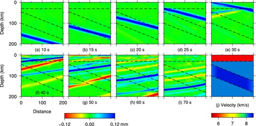
Fig. 17 shows the iteratively updated Moho discontinuity topography and Vp models through inversions of successively shorter period waveform data. Indeed, Moho topography is almost fully recovered by the 10 s and 6.25 s data (see the inverted Moho represented as the white curve and the actual Moho as the black curve in Model 5 of Fig. 17b). However, the two-layer slab, especially its thin low-velocity top layer, is much less well imaged by data up to 6.25 s because the thickness of the top layer, 14 km, is much shorter than the wavelength of 6.25 s P and S waves in the mantle (∼ 50 km and 28 km). Only a very weak fast-velocity anomaly (∼3 per cent) in the bottom layer emerges after 6.25 s inversions (Model 5 in Fig. 17b), probably thanks to the 37 km thickness of the faster bottom layer, which is more comparable to the wavelength of 6.25 s S waves in the mantle (28 km). Short-period data are obviously critical in refining structures and obtaining true amplitudes of the slab anomalies.
Iteratively updated Moho and Vp structures obtained by successive inversions of (a) 10 s, (b) 6.25 s, (c) 5 s, (d) 4 s and (e) 2.5 s waveforms. The white curves represent the inverted Moho, while the solid black curves denote the true Moho topography. The two-layer subducted slab is outlined by black dashed lines.
The subsequent inversions of 5 and 4 s data gradually reveal the slow top layer of the slab (Figs 17c and d), as the wavelength of 4 s S wave in the mantle (18 km) approaches the thickness of the top layer (14 km). However, artefacts around the Moho and in the upper crust (Model 8 in Fig. 17d) still persist, maybe owning to the trade-off between variations in Moho depth and volumetric parameters. To refine slab structures and reduce these artefacts, 2.5 s waveform data are further inverted. After another eight iterations, the artefacts fade away, and the slow anomalies on the top and fast anomalies on the bottom (Model 8 in Fig. 17e) layer of the slab are well constrained within the assumed regions. We take the density, Vp, Vs and Moho depth model of the last iteration of 2.5 s waveforms as our final model (Fig. 18). The amplitudes of the recovered density, Vp and Vs anomalies are close to −6 per cent and 4 per cent, which are the values that were used to construct the top and the bottom layers of the slab. Minor weak artefacts in the vicinity of the Moho are still visible in the final density (Fig. 18a) and Vs (Fig. 18c) models, the reduction of which may require further inversions of shorter period data, and/or more events for wider illumination angles.
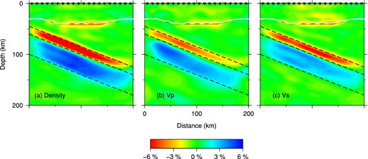
Final density (a), Vp (b) and Vs (c) models after a total of 32 iterations. The white curves denote the location of the inverted Moho, while the black solid curves denote the true Moho topography. The two-layer subducted slab is outlined by the black dashed lines.
Overall, a total of 32 iterations are performed in the whole inversion process for various period bands. Figs 19(a)–(c) and (g)–(i) show the horizontal and vertical displacement seismograms of an event with an incidence angle of 18° for the target model, the initial two-layer model m0, model m23 from the 23-rd iteration (the final model of 4 s inversion, i.e. Model 8 in Fig. 17d), and model m31 from the 31-st iteration (the final model of 2.5 s inversion, i.e. Model 8 in Fig. 17e). The station is located at x = 95 km, and the cut-off period of these seismograms is 2.5 s. The differences between the seismograms for the target model and three other models are displayed in Figs 19(d)–(f) and (j)–(l). Clearly, waveform misfits for successive models (m0, m23 and m31) are significantly reduced, both for the direct P waves and coda phases. The synthetics for the final model match those of the target model almost exactly. The evolution of the misfit value in the hierarchical waveform inversion process is shown in Fig. 19(m). Significant reduction is achieved in each iterative inversion process of a particular period-band data.
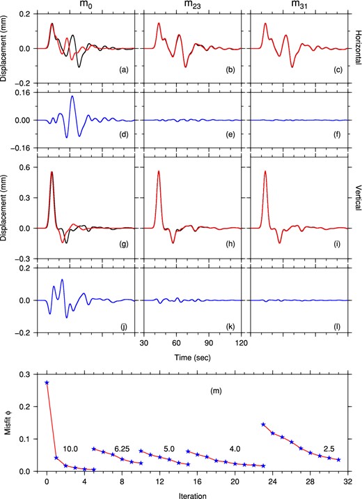
Comparison of horizontal (a–f) and vertical (g–l) component displacement seismograms in the starting model, m0 (left-hand panel), the final model of the 4 s waveform inversions, m23 (middle panel) and the final model, m31 (right-hand panel). The differences between the synthetic data for the target model (black traces in a–c, g–i) and the synthetic seismograms for iteratively updated models (red traces) are shown as blue traces (d–f, j–l). These seismograms are generated for an event with a P incidence angle of 18° and recorded at x = 95.0 km on the surface. (m) Iterative reduction of the misfit function value for 10, 6.25, 5.0, 4.0 and 2.5 s waveform inversions. The unit of the misfit function is 10−6 s m2.
For a complicated subduction zone model that includes a depression in the Moho and a lower velocity subducted oceanic crust atop a fast subducted lithospheric mantle, more sophisticated hierarchical inversion techniques have to be employed to ensure the approximate linearity of waveform misfits. Therefore, this synthetic example not only demonstrates a successful application of high-resolution array imaging by the teleseismic main phase and coda waves based on an SEM-FK hybrid method but also serves as another reminder of the high non-linearity of the inverse problem itself and the importance of carefully designed inversion strategies (e.g. Liu & Gu 2012).
5 DISCUSSIONS AND FUTURE WORKS
The SEM-FK hybrid method developed in this study provides a tool for the application of adjoint tomography to teleseismic converted/scattered wave imaging of crust and upper-mantle structures beneath seismic arrays. The interfacing of analytical wavefields for 1-D background models and numerically calculated full wavefield for 2-/3-D inhomogeneous media alleviates us from the currently prohibitively expensive computation of global seismic wave propagation at frequencies relevant to high-resolution array imaging. This cost limitation will of course become less stringent with the future evolution of supercomputer technology, but there is no hope of being able to use full 3-D simulations globally for inverse problems at such high frequencies before at least a decade, maybe even two. The response of local anomalies to incoming plane waves is accurately captured by the SEM-FK hybrid method that we have introduced. The planar incident wavefront assumption is valid at regional scales of several hundreds of kilometres (e.g. Rondenay et al.2008), hence applicable to most seismic array deployments.
Adjoint tomography based on the SEM-FK hybrid method is advantageous over traditional RF type of techniques (including migration methods such as CCP stacking) in several aspects. First, RF studies that obtain point estimates of the Moho depth assume a flat Moho (Zhu & Kanamori 2000) and may produce biased estimates for regions with large variations in Moho topography (Rondenay 2009), while CCP stacking methods generally assume a smoothly varying 1-D background model and are only capable of mapping out discontinuities. In comparison, adjoint tomography based on an SEM-FK hybrid method computes the forward and adjoint wavefields numerically, thus avoiding ray approximation and making no limiting assumption on the Moho geometry and background model. Therefore, it potentially allows for the use of 2-/3-D heterogeneous models, determined by traditional body- and surface wave methods, as initial models, thus reducing the non-linearity of waveform misfit and the trade-off between Moho variations and velocity perturbations. Secondly, adjoint tomography accurately calculates sensitivity kernels for converted and scattered waves that map inaccuracies of density, Vp, Vs and Moho topography in the current model, without the necessity of individual phase identification. The formal iterative optimization process sharpens models successively to fit the traveltime and waveform of both the main phase (e.g. P) and coda waves. In the two-layer subducted slab example (Section 4.3.2), discontinuity topography, density, Vp and Vs are updated simultaneously. Both structures and true amplitudes of the slab anomalies are well recovered in 32 iterations.
The use of inverse scattering techniques (such as the Generalized Random Transform) has made it possible to produce more physical images of density, Vp and Vs variations compared to reflectivity images from RF migration methods (Beylkin 1985; Bostock & Rondenay 1999; Rondenay et al.2008). However, the sparse and uneven distribution of sources (or incident angles) and receivers degrades the accuracy of the amplitudes of the density, Vp and Vs images. The wave-equation pre-stack depth migration method developed by Shang et al. (2012) cross-correlates the reverse-migrated P- and S-wave components, where reverse-time migration is performed by a FD calculation and allows heterogeneous background model and variations of interfaces, hence superior to CCP stacking for complex geological environments. However, it is effectively a one-step inversion, and the use of correlation between only P and S components places stringent requirements on receiver spacing (∼1/5 of the wavelength of the S wave), thus limiting its applicability in the case of most seismic arrays in practice (Shang et al.2012). Examples in our study show that with an SEM-FK hybrid method and adjoint techniques, receiver spacing may range from one to six times the dominant S-wave length to achieve waveform convergence, depending on the complexity of target models. Therefore, adjoint tomography based on an SEM-FK hybrid method can be readily used for imaging in most seismic arrays.
Adjoint tomography based on SEM-FK methods for converted/scattered waves, similar to all waveform inversion problems, is prone to entrapment in local minima, and designing proper inversion strategies that ensures that the process reaches the global minimum remains challenging. Our study shows that scaled product of sensitivity kernels for different coda phases provide a good pre-conditioner to preferentially update regions indicated by all phases. The combination of finite-frequency traveltime inversion of the main phase and waveform inversion of coda waves helps determine both long- and short-wavelength structures. Hierarchical inversions from long- to short-period waveforms reduce non-linearity at each stage, and by speeding up convergence, significantly reduce the numerical cost of 2-/3-D inversions. Other pre-conditioners and practices that are popular in the field of full-waveform inversion (e.g. Virieux & Operto 2009) could be exploited as well.
Although seismic waves propagation at local scales requires either 2.5-D (Roecker et al.2010) or 3-D (Komatitsch et al.2004) modelling, and seismic array are rarely precisely linear, we believe that our exhaustive 2-D synthetic tests in this study could provide useful guidance for future applications of more realistic 2.5- or 3-D modelling of teleseismic data. Our future work will focus on (1) application of 2-D SEM-FK adjoint tomography to realistic seismic array data in the 2.5-D framework (Roecker et al.2010; Zhou et al.2012; Xiong et al.2013; Pageot et al.2013), (2) extension of implementation and application to the 3-D case and (3) inclusion of seismic anisotropic structural parameters that provide possible clues to tectonic fabric and mantle flow patterns. Meanwhile, challenges posed by the estimation of source-time functions of the incident field, as well as the effects of noise in recorded scattered waves need to be carefully addressed in real applications. All these efforts should make adjoint tomography based on the SEM-FK hybrid method a useful tool in high-resolution imaging of tectonically and geodynamically complex regions beneath dense seismic arrays in the near future.
6 CONCLUSIONS
We have developed and implemented an SEM-FK hybrid method that interfaces FK solutions for 1-D background media with accurate SEM simulations of plane-wave propagation in 2-D local media. It takes into account complex wave phenomena associated with interactions of incoming teleseismic wavefield with local heterogeneities. The much smaller local computational domain permits the application of SEM for high-frequency body waves (∼1 s) with modest computational resources. The Fréchet kernels constructed based on the hybrid method naturally take into account the finite-frequency effect of seismic wave. Adjoint tomography that employs SEM-FK methods for forward calculations provides a powerful high-resolution imaging tool for teleseismic converted/scattered waves beneath seismic arrays. A non-linear CG method is used for the adjoint tomography to avoid the costly computation of the Hessian matrix. Our 2-D synthetic examples show promising results of this technique in determining density, Vp and Vs anomalies of the size of the dominant wavelength of S waves and with a magnitude of up to ±6 per cent, as well as large Moho variations. Combination of traveltime and waveform inversions is ideal in recovering both the long- and short-wavelength structures while keeping the inverse problem in the quasi-linear regime. For tectonically complex regions (e.g. subduction zones), we have used a hierarchical strategy from long to short periods to deal with the very non-linear character of waveform misfits, and we have successfully recovered both volumetric anomalies and Moho variations. These effective inversion strategies, together with the SEM-FK hybrid method, pave the way for future high-resolution regional imaging based on realistic seismic array recordings.
This research was supported by the G8 Research Councils Initiative on Multilateral Research Grant and the Discovery Grants of the Natural Sciences and Engineering Research Council of Canada (NSERC). Computations for this study were performed on hardware purchased through the combined funding of Canada Foundation for Innovation (CFI), Ontario Research Fund (ORF) and University of Toronto Startup Fund, and partly hosted by the SciNet HPC Consortium. SciNet is funded by CFI under the auspices of Compute Canada, the Government of Ontario, ORF-Research Excellence and the University of Toronto. We thank the developers of the SPECFEM2D package for their continued community support. We also thank Stéphane Rondenay, Jeroen Tromp and Shu-huei Hung for their helpful comments and suggestion. We are grateful to Dr Andrea Morelli and two anonymous reviewers for their critical comments and suggestions that have improved the original manuscript. Many figures were made with the Generic Mapping Tools (GMT; Wessel & Smith 1991).
