


Abstract
We study a minimal model of self-propelled particle in a crowded single-file environment. We extend classical models of exclusion processes (previously analyzed for diffusive and driven tracer particles) to the case where the tracer particle is a run-and-tumble particle (RTP), while all bath particles perform symmetric random walks. In the limit of high density of bath particles, we derive exact expressions for the full distribution  of the RTP position X and all its cumulants, valid for arbitrary values of the tumbling probability α and time n. Our results highlight striking effects of crowding on the dynamics: even cumulants of the RTP position are increasing functions of α at intermediate timescales, and display a subdiffusive anomalous scaling
  independent of α in the limit of long times
  . These analytical results set the ground for a quantitative analysis of experimental trajectories of real biological or artificial microswimmers in extreme confinement.
Export citation and abstract BibTeX RIS

Original content from this work may be used under the terms of the Creative Commons Attribution 3.0 licence. Any further distribution of this work must maintain attribution to the author(s) and the title of the work, journal citation and DOI.
1. Introduction
Stemming from experimental observations of bacterial motion [1], run-and-tumble particles (RTPs) provide a canonical model for the theoretical description of biological or artificial self-propelled entities such as Janus particles, bacteria [1–5], algae [6], eukaryotic cells [7], or larger scale animals [8]. In these examples of so-called active particles, self-propulsion results from the conversion of energy supplied by the environment into mechanical work [9, 10]. In its simplest form, RTP trajectories consists of a sequence of randomly oriented 'runs'—periods of persistent motion in straight line at constant speed—interrupted by instantaneous changes of direction (also named polarity of the RTP), called 'tumbles', occurring at random with constant rate.
The interplay between active particles and their environment has attracted significant interest recently [10]. Indeed, most motile biological systems such as bacteria or mammalian cells navigate disordered and complex natural environments such as soils, soft gels (e.g., mucus or agar) or tissues. Through their interactions with the environment, RTPs display robust non-equilibrium features, focus of many works. For example, recent simulations explored the dynamics of active particles in the presence of quenched disorder as well as active baths [11–15]. In confined geometries, active particles were found to accumulate at the boundaries, at odds with the equilibrium Boltzmann distribution [16–21]. Such non-trivial interactions with obstacles can lead to effective trapping and thus have important consequences in the dynamics of self-propelled particles in disordered environments [22]. For example, it was recently shown that the large scale diffusivity of RTPs moving in a dynamic crowded environment is non-monotonic in the tumbling rate for low enough obstacle mobility in dimension d ≥ 2 [23].
Effects of crowding are known to have particularly strong consequences in one-dimensional systems. In the classical example of single-file diffusion, where identical passive particles diffuse on a line, hard-core interactions impose conservation of the ordering of particles, thereby inducing long lived correlations in the motion of a tagged particle and eventually a subdiffusive scaling of its mean squared displacement,  with time n [24–32]. Physically, this results from the fact that displacements on increasingly large distances need to mobilize the motion of an increasingly large number of particles. Single file diffusion has been experimentally observed in a variety of natural and man-made materials ranging from passive rheology in zeolites [33, 34], transport of colloidal particles under confinement [35–39], to diffusion of water in carbon nanotubes [40, 41].
Diffusion under extreme confinement is also seen in biological settings with examples ranging from DNA translocation [42, 43], transport of proteins in crowded fluids like the cytoplasm [44], transport of ions in membrane channels [45, 46] and even migration of dendritic cells in lymphatic vessels [7]. Theoretically, recent works have studied the dynamics of active and biased tracer particles in single-file systems [47–50]. Exact predictions for the full distribution of particle positions were derived in the case of a tracer particle driven out of equilibrium by external forcing in a dense single-file environment [51]. Despite few effort, analytical results for the dynamics of self-propelled particles in complex and confined environments are still largely missing.
In this paper, we study a minimal model of self-propelled particle in a crowded single-file environment. Despite the challenge of the inherent coupling between the dynamic environment of the tracer and its polarity, we derive exact analytical results for the dynamics of RTP in the limit of high density of diffusive bath particles; in particular, we provide expressions for the full distribution  of the RTP position X and all its cumulants, valid for arbitrary values of the tumbling probability α and time n. Our results highlight striking effects of crowding on the dynamics. We show in particular that even cumulants of the RTP position are increasing functions of α at intermediate timescales, and display a subdiffusive anomalous scaling
  with a prefactor independent of α in the limit
  . We show a perfect agreement between our analytical predictions and the results of numerical simulations. We generalize to RTPs questions that have attracted attention for passively diffusing and externally driven tracers. In section 2, we provide the details of our model. The more technical sections 3 and 4 detail the necessary steps in the derivation of our main results presented in equations (16) and (19) which we discuss respectively in sections 5 and 6. Additional technical details of this derivation can be found in Appendices.
2. Model and RTP polarity dynamics
We consider a minimal model of run-and-tumble motion [1] discrete both in space and in time. We take a one-dimensional lattice, infinite in both directions. The lattice sites are occupied by particles with mean density ρ performing symmetric random walks; the bath particles interact via hard-core repulsion, i.e. the occupancy number of each lattice site is at most equal to one. At time n = 0, we place at the origin a RTP, which also interacts with the bath particles via hard-core repulsion. In absence of bath particles, the RTP moves along the direction of its polarity with probability  , and in the opposite direction with probability
  such that
  . At each time step, the RTP reverses the direction of its polarity with probability α.
While previous studies examined the dynamics of externally driven tracers [51, 52], we are interested here in a model of internally driven self-propelled particles with an internal clock. Although in general  can take any value between 0 and 1, we consider the limit of a self-propelled particle with infinite Péclet number [10]. Thus, if its polarity is along
  (respectively,
  ), the RTP moves to its right with probability p1 = 1 and to its left with probability p−1 = 0 (respectively, p1 = 0 and p−1 = 1). In the absence of crowders, this model would produce a dynamics equivalent to a persistent random walk.
We focus here on the limit of dense systems, i.e. the limit of low vacancy densities ρ0 = 1 − ρ ≪ 1. Following [53], we formulate in this limit the dynamics of the vacancies rather than that of the particles which equivalently encodes the dynamics of the whole system. We follow the evolution rules for the vacancies previously established by [51, 53–55] in which we assume that each vacancy performs a nearest-neighbor symmetric random walk everywhere on the lattice except in the vicinity of the RTP [56]. When surrounded by bath particles, a vacancy thus moves to one of its neighboring sites with equal probability, thereby exchanging positions with a bath particle. However, when the RTP lies on one of its adjacent sites, we accommodate the nature of the RTP dynamics by implementing the following specific rules (as shown on figure 1):
- if the vacancy occupies the site to the right of the RTP, the vacancy has a probability
 to jump to the right (exchanging positions with a bath particle) and to jump to the left (exchanging positions with the RTP);
 - if the vacancy occupies the site to the left of the RTP, the vacancy has a probability to jump to the left (exchanging positions with a bath particle) and to jump to the right (exchanging positions with the RTP).


For instance, in the case of a RTP with positive polarity (i.e. polarity along  ), we know that p1 = 1 and p−1 = 0; thus, we obtain in this case q1 = 1/3 and q−1 = 1. The case of a negative polarity can easily be deduced by symmetry. It is important to note that additional rules for the cases where two vacancies are adjacent or have common neighbors would normally be needed to complete the description of the dynamics; however, these cases lead to corrections in
  and are thus unnecessary here. Although these hopping probabilities implicitly depend on the RTP polarity at a given time, the decoupling between the dynamics of the polarity and the vacancies makes analytical calculations tractable.
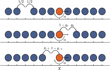
Figure 1. Model and evolution rules—The RTP (orange) moves through a bath of diffusive particles (blue), its polarity flips at each time step with probability α; the RTP moves by exchanging positions with vacancies. We formulate this problem in terms of the dynamics of the vacancies rather than that of the particles. A vacancy can (i) be surrounded by bath particles, (ii) have the RTP on its left, (iii) have the RTP on its right. Here, the RTP is polarized to the right, so that q1 = 1/3 and q−1 = 1.
Download figure:
Standard image High-resolution imageIndeed, the polarity dynamics of the RTP is solely controlled by its flipping probability α. We will denote  the probability for the RTP to have a given polarity μ at time step k, knowing that it was ν at k = 0. For all times k assuming that we started with a positive polarity, we can write the following recurrence relation
  . Using the method of fixed-points to solve this recurrence relation, we obtain for a polarity μ,

For the sake of simplicity, we may write  and
and  in what follows.
3. Systems with a single vacancy
Following [54], we first consider an auxiliary problem: a system containing a single vacancy. We consider a lattice on the integers l ∈ [−L; L], the vacancy can occupy any site but the origin. We can write the probability to find the RTP in position X at time n, knowing it started with polarity ν at time n = 0 as an average over the initial condition for the position of the vacancy Z,

with  defined as the probability to find the RTP in position X at a time n knowing its polarity was initially ν and that the vacancy started in Z. Trivially in the single vacancy case, the RTP can only be in one of two positions which depend on the original location of the vacancy: if the vacancy starts in Z > 0 (respectively, Z < 0), the RTP can be found in X = 0 or X = 1 (respectively, in X = −1 or X = 0). The dynamics of the RTP is dictated by exchanges of positions with the vacancies, as such it is controlled by the first-passage statistics of vacancies to the position of the RTP. Clearly, there are four cases to consider in general, but symmetry considerations reduce those cases to two: for a given initial RTP polarity, the vacancy can start (1) in front of the RTP or (2) behind the RTP with respect to the direction of its polarity.
We can represent  as a sum over all passage events of the vacancy to the RTP location through the following recurrence relation [51, 53, 55]

with  the probability that the vacancy starting in Z exchanged position with the RTP in time n knowing that it started with polarity ν and sgn(x) the sign function taking values in {−1; 1 }. In equation (3), the first term on the right-hand side corresponds to the probability that the RTP has not moved, while the second term is composed of a convolution between the probability to have exchanged positions in k steps and the probability that the RTP travels the remaining X − sgn(Z) steps in time n − k; in particular, we know that this probability needs to be written with a polarity sgn(Z) and that the vacancy now starts in −sgn(Z) (vacancy and RTP exchanged positions). We note that the single vacancy propagator only depends on
  and the propagator in the case of a vacancy starting right next to the RTP. We denote
  the first-passage time (FPT) density in X = 0 for a vacancy starting in μ = ±1, knowing that the RTP started with a polarity ν at n = 0. By symmetry, we know that we can write:


In particular, we notice that  can be written as the convolution of the FPT density of a Pólya walk to the adjacent site to the RTP and this FPT density of exchange of RTP and vacancy position, for a vacancy starting on one of the lattice sites adjacent to the RTP. We thus write

where  denotes the classical FPT density at the origin at time n of a symmetrical one-dimensional Pólya walk starting at n = 0 at position X [56] and
  the probability for the RTP to have a given polarity μ at timestep n, knowing that it was ν at n = 0 for which it is straightforward to obtain exact expressions (as introduced in section 2). The two terms in equation (6) correspond to the two possible polarity states of the RTP at time k. In the particular case of a vacancy starting in μ = ±1, this probability reads (see detailed calculation for each of the cases in appendix A)

with δi, j the Kronecker delta. The first term in the right-hand side of equation (7) gives the probability that at time n the RTP was never visited by the vacancy. The second term represents a partition over the number of visits by the vacancy j and the waiting times between successive visits mj and a last non-visiting event. Here, the key step of our derivation is therefore to compute the FPT densities  which a priori couple the polarity dynamics and vacancy dynamics. Thanks to the Markovian dynamics of the RTP polarity, we obtain exact full expressions for these FPT densities and their generating functions as shown in appendix B. For instance, we show that
  obeys the following recurrence relation
At each time step, the RTP (i) flips its polarity with probability α and (ii) attempts to make a step in the direction of its polarity. The first term in equation (8) corresponds to the case where the RTP does not flip its polarity at n = 1. In this case, we know that the RTP has a chance to exchange positions with the vacancy at n = 1 (this is the first term in the curly brackets), the second term is based on the probability that the vacancy did not exchange positions with the RTP at n = 1 but came back in  steps while the polarity is still positive, and the third term is based on the probability that the vacancy did not exchange positions with the RTP at n = 1 but came back in k − 1 steps while the polarity flipped in the meantime. The second term in equation (8) corresponds to the case where the RTP does flip its polarity at n = 1. This case is similar to the first term, with the exception that we know that the RTP and the adjacent vacancy cannot exchange position at the first time step.
Defining the generating function of any time-dependent function g(n) as  , equations (3)–(7) imply that the generating function of the single-vacancy propagator can be written in terms of the generating functions of the FPT densities above as

where we have used the short-hand notations  and the original position of the vacancy, μ = ±1 (see details in appendix A).
4. Systems with a small concentration of vacancies
We now consider a lattice containing a low concentration of vacancies ρ0; we assume that the lattice of size  contains M vacancies such that
  . First, we consider the case of a fixed initial polarity for the RTP, ν. Following [53], we write
  the probability that the RTP with original polarity ν is at position X at time n provided that the M vacancies started at positions
 ![${\{{Z}_{j}\}}_{j\in [1,M]}$](https://content.cld.iop.org/journals/1367-2630/20/11/113045/revision2/njpaaef6fieqn40.gif) . At the lowest order in the vacancies density, we consider the contributions of each vacancy to be independent and we write
. At the lowest order in the vacancies density, we consider the contributions of each vacancy to be independent and we write

where  is the conditional probability that in time n the RTP has performed a displacement Y1 due to interaction with the vacancy 1, Y2 due to interaction with the vacancy 2 etc. We define the Fourier transform in space as
  , where the sum runs over all lattice sites. In Fourier space and averaged over the initial distribution of vacancies positions (assumed to be uniformly distributed on the lattice, except for the origin which is occupied by the RTP, and denoted with a bar), the total contribution of the M vacancies reduces to a superposition of the contributions of single vacancies providing us with a formal relationship between the general propagator and the single vacancy propagator

where we impose  (while ρ0 is kept constant) and we define

Lastly, we average over the initial polarity of the RTP to obtain

with ![${\rm{\Omega }}(q,n)\equiv [{{\rm{\Omega }}}_{+}(q,n)+{{\rm{\Omega }}}_{-}(q,n)]/2$](https://content.cld.iop.org/journals/1367-2630/20/11/113045/revision2/njpaaef6fieqn44.gif) . The generating function of the second characteristic function, which is defined as
. The generating function of the second characteristic function, which is defined as  , satisfies the following relation

After lengthy but straightforward algebra (see details in appendices C and D), we proceed to an expansion of  in power series of q to obtain

We now have all the tools to derive our central analytical result which defines the exact (in the leading order in ρ0) cumulant generating function. The cumulants κj of arbitrary order j are defined by ![$\mathrm{ln}[{\bar{P}}^{* }(q,n)]\equiv {\sum }_{j=1}^{\infty }{\kappa }_{j}^{(n)}{({\rm{i}}{q})}^{j}/j!$](https://content.cld.iop.org/journals/1367-2630/20/11/113045/revision2/njpaaef6fieqn47.gif) . We can identify equal order terms in both expressions and find
. We can identify equal order terms in both expressions and find

Recalling that the FPT densities  are explicitly given in appendix B in terms of the tumbling probability (appearing explicitly through the Poissonian dynamics of the polarity), equation (16) provides an expression for all cumulants exact in the leading order in ρ0 in Laplace space. Equation (16) together with its asymptotic analysis in equations (17) and (18) constitute the main result of this paper. Strikingly, all cumulants of same parity are equal and in particular, all odd cumulants are identically equal to 0. While we easily understand why odd cumulants in a process averaged over the initial polarity should be zero, it is interesting to note that in the case where we fix the initial polarity of the RTP, the odd cumulants were non-zero but decaying as
  (see appendix C.4). As a side note, we show in appendix C.5 that our predictions retrieve the results for the infinitely biased tracer particle in the α → 0 limit [51].
5. Cumulants in the long-time limit
We expand the generating function of the even cumulants in power series of 1 − ξ (which is equivalent to a long-time limit expansion)

Using Tauberian theorems [57], we can invert term by term this expression and we obtain in the time domain

From equation (18), we first notice that the leading asymptotics are surprisingly independent of the tumbling probability α. In figure 2, we show that the mean-square displacement of the RTP converges in the long-time limit to the anomalous subdiffusive scaling observed for passive single-file diffusion. This comes from the fact that, for all finite values of α, the statistics of the waiting times between successive steps of the RTP is asymptotically independent of α. Secondly, by obtaining higher order terms in the expansion of the cumulants, we realize that α enters in the first subleading order term with the expected monotonicity. As shown in figure 3, as the tumbling probability decreases (i.e. the more persistent the RTP becomes), the importance of the higher order terms in the expansion decreases and the dynamics of the RTP converges faster to the classical single-file scaling.

Figure 2. Mean square displacement of the RTP—shown for various tumbling probabilities α ∈ [0.01; 0.5] showing an α-dependent transient to a subdiffusive long-time scaling independent of α; at long times,  (dashed black line).
Download figure:
Standard image High-resolution image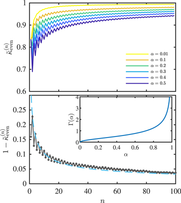
Figure 3. Reduced cumulants—(Top) Reduced cumulants  versus time n for several tumbling probabilities, showing transients dependent on α (increasing α from yellow to blue) obtained from the inversion of equation (16); (Bottom) Reduced cumulant for a tumbling probability α = 0.3 and a vacancies density of ρ0 = 0.001, from inversion of equation (16) (solid line), numerical simulations (symbols) and first higher order term in the Taylor series of the cumulants as in equation (18) (dashed line),
  . The α-dependance of the higher-order term is shown in inset.
Download figure:
Standard image High-resolution imageSurprisingly, we observe that the time-averaged MSD decreases faster for smaller α for short timescales t ≪ 1/α (see figure 2). This counterintuitive result is opposite to the monotonicity expected in the absence of obstacles. After this transient, one recovers the expected monotonicity of the MSD with respect to tumbling probability for t ≫ 1/α. Thus, the time-averaged stationary mean-square displacement (figure 2) shows an inversion of monotonicity of the second cumulant compared to that of the ensemble-averaged cumulants (figure 3) in the n → 0 limit, a common signature of aging phenomena. Namely, this result suggests that the stationary distribution of vacancy positions is different from the Poissonian initial conditions we consider in the derivation leading to figure 3. Indeed, the bath particles density displays fluctuations in the vicinity of the RTP (with an increase of particles density in front of the RTP and a decrease at the back). This implies that a higher persistence can lead to a slowing down of the dynamics at short timescales, a counterintuitive idea reminiscent of the concept of negative differential mobility observed for biased tracers and RTPs in crowded environments [23, 52, 58].
6. Full statistics of the RTP position
Finally, the equality of same parity cumulants (to leading order in ρ0) implies that the associated distribution is of Skellam type, i.e. the distribution of the difference of two Poissonian random variables [59]. As a consequence, our results provide the complete distribution of RTP positions  for any time n, which in our case simplifies to

where IX is a modified Bessel function of the first kind [60]. Figure 4 shows a perfect agreement between the predicted distributions and our numerical simulations. In the long time limit, we recover the results derived by [25] and [61]. The expression for the distribution of positions reduces to

Importantly, we find that independently of the tumbling probability the rescaled variable  is asymptotically distributed according to a normal law.

Figure 4. Distribution of positions of a RTP with random initial polarity  , tumbling probability α = 0.2 and vacancy density ρ0 = 0.01 for various times n = 103, 104, 105 and 106 (from yellow to blue), for numerical simulations (symbols) and theoretical predictions obtained from equation (19) (solid lines).
Download figure:
Standard image High-resolution image7. Conclusion
Using a lattice model, we derived expressions for the full statistics of positions of RTPs with arbitrary tumbling probability α in dense single-file environment. Our predictions are exact to the leading order in vacancy density ρ0 → 0. We have shown that the asymptotic dynamics of the RTP displays an anomalous subdiffusive scaling  with prefactor independent of α. Further, we highlighted the presence of aging in this system for which the stationary distribution of bath particles is not Poissonian but displays density fluctuations in the vicinity of the RTP leading strikingly to a slowing down of the short timescale dynamics for more persistent RTPs. RTPs are a canonical model of natural and artificial self-propelled particles; as a consequence, we believe that these exact results will find a wealth of applications; they set the ground for a quantitative analysis of experimental trajectories of real biological or artificial microswimmers in extreme confinement.
Appendix A.: Single vacancy propagator
In this appendix, we provide details about the calculation of the single vacancy propagator. First, we consider the case where Z > 0 and the RTP started with a positive polarity at n = 0. We can write the following recurrence relation:

with  the probability that the vacancy starting in Z exchanged positions with the RTP in time n knowing that its polarity was + at n = 0. In particular, we notice that
  can be written as the convolution of the FPT density of a Pólya walk to the adjacent site to the RTP and the FPT density of exchange of RTP and vacancy position, for a vacancy starting on one of the lattice sites adjacent to the RTP knowing the polarity of the RTP.

where  denotes the FPT density at the origin at time n of a symmetrical one-dimensional Pólya walk starting in position X at n = 0 and
  is the FPT density of exchange of the positions of the RTP and the vacancy in time n, knowing that the RTP started with an initial polarity ν and the vacancy started in Z = μ1. Full expressions for those FTP densities are derived in appendix B. We note that we have similarly

In equation (A.1), the first term corresponds to the probability that the RTP has not moved and the second term is composed of a convolution between the probability to have exchanged positions in k steps and the probability that the RTP travels X − 1 steps in time n − k, granted that it had a polarity + at n = 0 and that the vacancy started now in −1 (vacancy and RTP exchanged positions).
Similarly in the case Z < 0, we have:

(in this expression the second term contains the probability  because we know that the propagator needs to be shifted following interaction with the vacancy coming from the left of the RTP and the fact that the polarity had to flip in order for the RTP and the vacancy to exchange positions).
By symmetry, we obtain similarly
As we can see from equations (A.1), (A.4) and (A.5), finding the general single vacancy propagator reduces to finding an expression for the single vacancy propagator in the case of a vacancy adjacent to the RTP. With some care, the general single vacancy propagator can be expressed using the first-passage statistics of the vacancy starting on a site adjacent to the RTP to its position. For instance, the probability to find the RTP in position X in time n knowing that the RTP started in X = 0 with a positive polarity and a vacancy in Z = +1 reads:
Equation (A.6) is composed of three terms:
- (i)the RTP is in 0, it was never visited by the vacancy;
- (ii)the RTP is in 0, it was visited an even number of times; this term contains visits and 1 last non-visiting event;
- (iii)the RTP is in 1, it was visited an odd number of times; this term contains visits and 1 last non-visiting event.


Taking the discrete Laplace transform of equation (A.6) and denoting the FPT densities  for the sake of simplicity, we find

which finally reduces to

Similarly, we find that
Taking the discrete Laplace transform of equation (A.9), we obtain:

By symmetry, we can write the remaining two cases


Finally, we realize that the single vacancy propagator only depends on the FPT densities  ,
,
We provide a full derivation of those quantities in appendix B.
Appendix B.: First-passage time densities for vacancies adjacent to the RTP
Knowing that the RTP polarity is in a given state at n = 0 and that a vacancy is adjacent to the RTP at that time, we want to calculate the probability that a first interaction (i.e. exchange of positions) will happen at time n. In all generality, there are four possible configurations to consider at n = 0 assuming that the RTP is in X = 0:
- RTP polarity is (+) and the vacancy is in X = +1;
- RTP polarity is (+) and the vacancy is in X = −1;
- RTP polarity is (−) and the vacancy is in X = +1;
- RTP polarity is (−) and the vacancy is in X = −1.
We denote  the FPT density in the case where the RTP polarity is originally ν and the vacancy started in Z = μ1. We will detail here the derivation on an example. We will consider that the polarity is positive at n = 0. Knowing that a vacancy is next to the RTP at n = 0, we want to calculate the probability of first interaction (exchange of positions) at time n. In this particular case, the vacancy has a chance to interact with the RTP at the first time step, and we can express this quantity via the FPT density at the origin at time n of a symmetrical one-dimensional Pólya walk starting at n = 0 at position l and denoted
  . Thus, we write the FPT density as the following convolution:
Similarly, for a vacancy starting on the left of the RTP with a positive polarity, we write
For a given vacancy position, the polarity of the RTP can be pointing towards the vacancy or not. By symmetry, we only need to compute these two cases. We denote  the FTP density for the case where the vacancy is on the right side of the RTP given its polarity, while we denote
  the inverse case and we have,


Furthermore, by definition, we can also write that  . For the sake of simplicity, we will define :


We can study the discrete Laplace transform of these two quantities, defined as:  . Using the convolution theorem, we obtain:


We can combine equations (B.7) and (B.8) to obtain finally


Going back to the definition of the discrete Laplace transform, we obtain the following expressions


with by definition of a Pólya walk:

As a conclusion, we have obtained exact expressions for the FPT densities we needed to complete our expression of the single vacancy propagator.
Appendix C.: Single file with a small concentration of vacancies
In this appendix, we consider the case of a small but finite concentration of vacancies, we assume that the system contains M vacancies such that  . We will start by deriving expression for the cumulants, exact in the linear order in the density of vacancies. We will then show that our results are consistent with the results in the case of a biased tracer particle (derived in [51]).
C.1. Case of a fixed initial polarity
First, we consider the case where we fix the initial polarity of the RTP. Following Brummelhuis and Hilhorst [53, 54], we write in general  the probability that the RTP is at position X at time n provided that the M vacancies were at positions
 ![${\{{Z}_{j}\}}_{j\in [1,M]}$](https://content.cld.iop.org/journals/1367-2630/20/11/113045/revision2/njpaaef6fieqn74.gif) and the RTP polarity was ν at n = 0. We can write:
and the RTP polarity was ν at n = 0. We can write:

where  is the conditional probability that, within the time interval n, the RTP has performed a displacement Y1 due to interaction with the vacancy 1, Y2 due to interaction with the vacancy 2 etc. In the lowest order of the vacancy density ρ0, the vacancies contribute independently to the displacement:

Thus, we can express this probability as a function of the single vacancy propagator:

If we suppose that the vacancies are uniformly distributed, we can average  over the initial distribution of vacancies:


By definition, the Fourier transform in space is written as:

where the sum runs over all lattice sites.
For the sake of simplicity and without loss of generality, we can assume that the polarity is always positive in n = 0. As a consequence of equation (C.6), the probability averaged over initial conditions for the vacancies reduces in Fourier transform to

From equation (A.13), we write in Fourier space:

We can rewrite equation (C.8) as:

where we define the following quantity

By definition of the Fourier transform for a random variable Xn :

The cumulant generating function, defined as  , reads in the limit of low vacancies density (ρ0 ≪ 1):

with  and
and  . This leads to the Z-transform relation:

By discrete Laplace transform, we obtain:

with  , we provide full calculation and expressions for these quantities in appendix C.2.
C.2. Calculation of

We have already noticed (in section 3 and appendix A) that:

The associated generating functions are thus simply:

In particular, we have


Finally, we can write that:

We can also write:

In conclusion, in general, we have:

C.3. Expression for the cumulants with positive initial polarity
From equations (A.10) and (A.11), the Laplace-Fourier transform of the single vacancy propagator is given by:


Combining equations (C.15), (C.22), (C.23) and (C.24), we finally obtain:
On one hand, we can proceed to the expansion of  in power series of q:
Recalling the definition of the generating functions of the cumulants  of arbitrary order j, we can write

So we can identify same order terms and write that:

Equation (C.28) provides an exact expression of the cumulants in the Fourier-Laplace space. Recalling that the functions  are explicitly given in appendix B in terms of the tumbling probability, this equation gives an expression of the cumulants of arbitrary order.
C.4. Cumulants in the long-time limit
From equation (C.28), we see that all odd cumulants have the same generating function  and all even cumulants have the same generating function
  . We recall that the expression for the
  is given by equations (B.9) and (B.10). We can thus proceed to an expansion in power series of 1 − ξ (which is equivalent to a long-time expansion in the time domain) of the generating function of the cumulants and using the fact that q1 = 1/3, we find that:


At this point, it is useful to remember the Tauberian theorem [57]. For a time-dependent function ϕ(n) and its associated generating function  , if the expansion of
  in powers of (1 − ξ) has the form

Then, the long time behavior of ϕ(n) is given by

where Γ is the usual gamma function. This relation holds if χ > 0, ϕ(n) > 0, ϕ(n) is monotonic and Φ is slowly varying in the sense that

for any λ > 0.
Using the Tauberian theorem, we find that the long-time behavior of the odd cumulants is given by

and a long-time behavior of the even cumulants given by

We note that remarkably the leading order in time of the even cumulants does not depend on α, while the leading order in time of the odd cumulants does and decays to zero in the long time limit. The asymptotic behavior of κeven(n) tells us that the variance of the RTP position grows as  , this subdiffusive behavior is the one obtained for the classical symmetric single file dynamics.
C.5. Retrieving the case of a biased tracer particle in the limit

For sanity, we can check our calculation against the result for a biased tracer particle (TP) [51]. In this section, we will check that our derivation for a run-and-tumble tracer particle in the limit α → 0 gives the same prediction as in the case of an infinitely biased TP. In particular, we recall that the cumulants of all order in the biased case are given by:

where  and q±1 defined as in the RTP case. In the case of an infinite bias, we know that q1 = 1/3 and q−1 = 1 leading to

In the run-and-tumble case, we need to first take the limit of low tumbling rate, α → 0, before taking the limit of long-times. Using equations (B.9) and (B.10) with q1 = 1/3, we can write the FTP densities as:


Injecting this result in equation (C.28), we obtain that for all orders:

We notice that: (1) cumulants in the infinitely biased case and the RTP case in the limit α → 0 are equal and (2) expressions for the cumulants for all orders are equal. This means that in all cases, all cumulants are equal and in particular, an expansion in power series of 1 − ξ gives:

Hence, we conveniently retrieve the biased case in the zero tumbling rate limit (α → 0).
Appendix D.: General case: random initial polarity
We generalize in this appendix our derivation to the case of a random initial polarity to obtain the cumulants and full statistics for the RTP position. For that, we need to average over trajectories conditioned with positive and negative initial polarity.
D.1. Cumulants in the case of a negative initial polarity
It is rather straightforward to calculate the specific case of a fixed negative polarity and check that it gives us the expected result considering the derivation in appendix C. Similarly to the previous derivation, we write in this case

From equation (A.13), we can write:

Following the same procedure and definition as in appendix C, the previous expression expanded reads

Finally the cumulants are given by identification of the nth order terms in the development, and we obtain:

Comparing equations (C.28) and (D.4), it is easy to see that these expressions will yield the same cumulants for all even orders, and cumulants with opposite signs for all odd orders.
D.2. Expression of the cumulants in the general case
The final step is now to average over the initial polarity, we condition on the polarity right after the averaging over initial conditions for a small concentration of vacancies. As such, we write:

Reinjecting in this expression equations (C.8) and (D.1), we obtain

with ![${\rm{\Omega }}(q,n)=[{{\rm{\Omega }}}_{+}(q,n)+{{\rm{\Omega }}}_{-}(q,n)]/2$](https://content.cld.iop.org/journals/1367-2630/20/11/113045/revision2/njpaaef6fieqn93.gif) when
when  . In the Laplace domain, we obtain then

i.e.

As usual, the expression for the cumulants is given by identification of the terms in the expansion and we get

As a conclusion, we can easily see that all even cumulants are equal, as are all odd cumulants. We obtain the following final cumulants


We realize that all odd cumulants are identically equal to 0. As for the even cumulants, they present the same form as the even cumulants in the case of a positive conditioning, which was expected as the initial polarity only affects the dynamics until the first polarity flip. We can proceed to a power series expansion of the generating function of the cumulants in  including the first non-zero subleading order term and we get:

This expression can be inverted term by term and we obtain in time domain

In particular, the second cumulant is by definition the mean-square displacement of the RTP. Although we can see that the transient depends on the tumbling probability, the MSDs display a  long-time scaling characteristic of the original single file process that is in particular independent of α.